Please complete this assignment using the RMarkdown file provided. Once you download the RMarkdown file please (1) include your name in the preamble, (2) rename the file to include your last name (e.g., “weston-homework-3.Rmd”). When you turn in the assignment, include both the .Rmd and knitted .html files.
To receive full credit on this homework assignment, you must earn 30 points. You may notice that the total number of points available to earn on this assignment is 65 – this means you do not have to answer all of the questions. You may choose which questions to answer. You cannot earn more than 30 points, but it may be worth attempting many questions. Here are a couple things to keep in mind:
Points are all-or-nothing, meaning you cannot receive partial credit if you correctly answer only some of the bullet points for a question. All must be answered correctly.
After the homework has been graded, you may retry questions to earn full credit, but you may only retry the questions you attempted on the first round.
The first time you complete this assignment, it must be turned in by 9am on the due date (December 8). Late assignments will receive 50% of the points earned. For example, if you correctly answer questions totaling 28 points, the assignment will receive 14 points. If you resubmit this assignment with corrected answers (a total of 30 points), the assignment will receive 15 points.
You may discuss homework assignments with your classmates; however, it is important that you complete each assignment on your own and do not simply copy someone else’s code. If we believe one student has copied another’s work, both students will receive a 0 on the homework assignment and will not be allowed to resubmit the assignment for points.
A helpful note: I recommend using the tidyverse function read_csv()to load datasets, not the base-R function read.csv(). I have found that this results in fewer weird table-problems.
Data: Some of the questions in this assignment use the dataset referred to as homework-school. This is a sample of Oregon students collected through the Census at School project. Non-numeric responses to numeric questions (e.g., “a lot” as a response to “How many hours per week do you text your friends?”) have been removed, but no other cleaning has been done. Be warned: missing values and implausible (and impossible) responses abound.
Other questions refer to the dataset homework-nls that contains the following variables from the National Longitudinal Survey of Youth 1997, collected in 2000 and 2010:
sex
calm_2000
blue_2000
happy_2000
depressed_2000
calm_2010
blue_2010
happy_2010
depressed_2010
Finally, we return once again to the World Happiness Survey, an attempt to track important issues in over 160 countries, representing about 99% of the world’s population. A small part of that survey is in the dataset homework-world-2. Included are the country name, country development status (First World, Second World, Third World, or Other), the life ladder score, and a binary happiness variable called Above_Average.
Calculate the effect size for the previous question.
Question 3
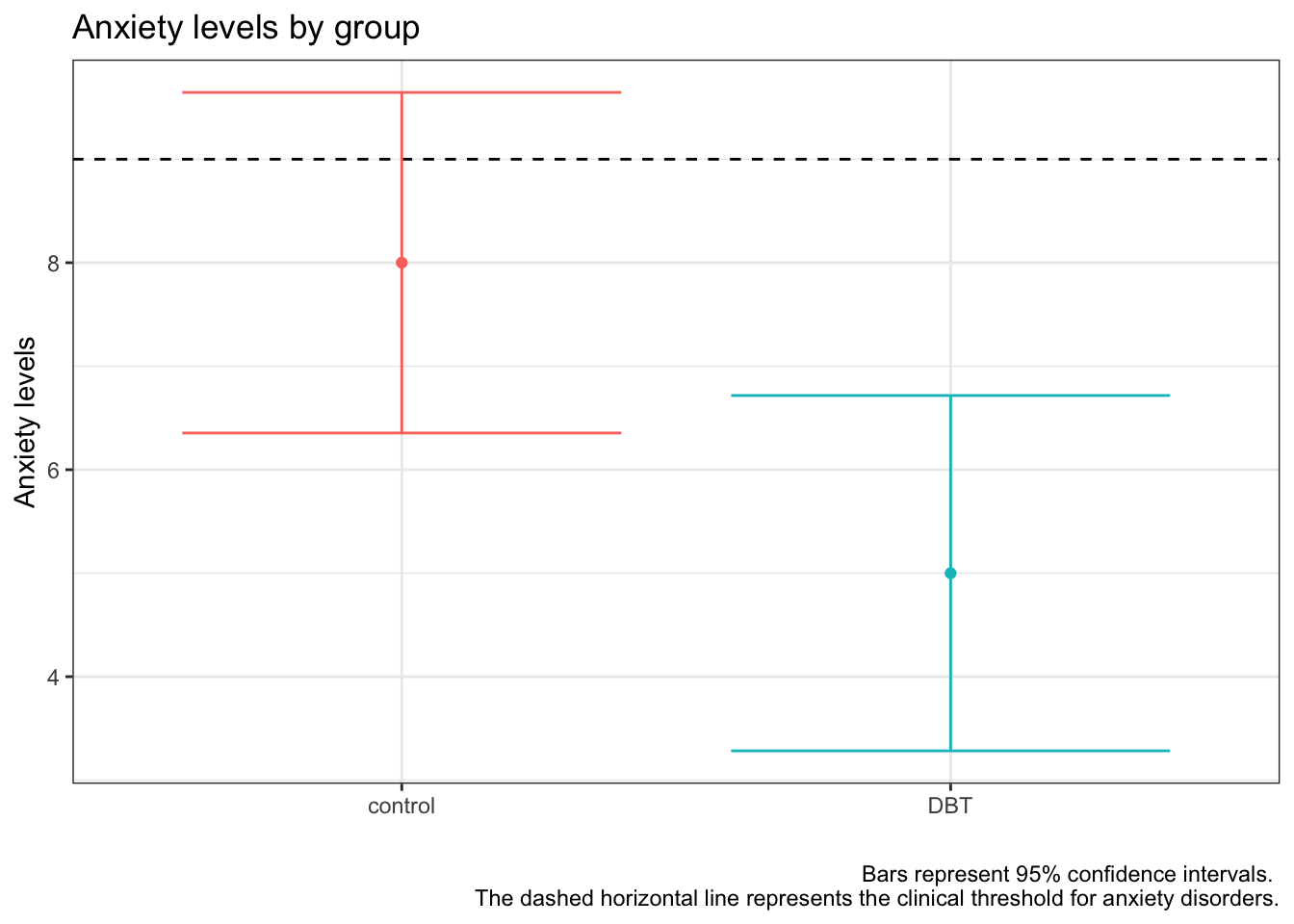
At a conference, you attend a talk about the effectiveness of a DBT therapy intervention on anxiety. The presenter puts up the figure below. The presenter claims that these groups are significantly different from one another, because the experimental group shows significantly lower anxiety than the clinical threshold, but the control group does not. Do you agree with thee presenter? Explain your answer.
data.frame(group =c("control", "DBT"),xbar =c(8, 5),s =c(2.3, 2.4), N =c(10, 10)) %>%mutate(se = s/sqrt(N),cv =qt(p = .975, df = N-1),moe = se*cv) %>%ggplot(aes(x = group, y = xbar, color = group)) +geom_point(stat ="identity") +geom_hline(aes(yintercept =9), color ="black", linetype =2)+geom_errorbar(aes(ymin = xbar-moe, ymax = xbar+moe), width = .8)+guides(color ='none')+labs(x ="", y ="Anxiety levels", title ="Anxiety levels by group",caption ="Bars represent 95% confidence intervals. The dashed horizontal line represents the clinical threshold for anxiety disorders.")+theme_bw()
Question 4
Daylight in Eugene winter is a precious commodity. You believe that undergraduates who live on the top floor of their dorm or apartment building are getting more sun (and more of that sweet, sweet Vitamin D) than students living on the bottom floors. You measure the amount of vitamin D in undergraduates blood streams and record the averages by where students live.
\(\hat{\mu}_{\text{TopFloor}}\) = 31 ng/mL
\(\hat{\mu}_{\text{BottomFloor}}\) = 26 ng/mL
\(\hat{\sigma}_{\text{TopFloor}}\) = 7.4 ng/mL
\(\hat{\sigma}_{\text{BottomFloor}}\) = 8.3 ng/mL
\(n_{\text{TopFloor}}\) = 20
\(n_{\text{BottomFloor}}\) = 23
Calculate the t-statistic for the difference between the two means. Assume the variances of the two groups are equal.
Is the difference between the two means significant? Use \(\alpha = .05\) and a two-tailed test. (Don’t forget to calculate the degrees of freedom.)
Question 5
Your collaborator thinks there’s a better way to test this question. He conducts a longitudinal study on bottom-floor residents, measuring blood Vitamin D levels one year, and then measures them again if they move to a the top floor the next year. Overall, he manages to measure Vitamin D twice in a group of 16 bottom-then-top floor residents.
\(\hat{\mu}_{\text{TopFloor}}\) = 31 ng/mL
\(\hat{\mu}_{\text{BottomFloor}}\) = 26 ng/mL
\(\hat{\sigma}_{\text{TopFloor}}\) = 7.4 ng/mL
\(\hat{\sigma}_{\text{BottomFloor}}\) = 8.3 ng/mL
\(n_{\text{TopFloor}}\) = 16
\(r_{\text{TopFloor,BottomFloor}}\) = 0.78
Calculate the t-statistic for the difference between the two means.
Is the difference between the two means significant? Use \(\alpha = .05\) and a two-tailed test. (Don’t forget to calculate the degrees of freedom.)
Do you agree that this way is better? What are the advantages and disadvantages of your collaborator’s method?
5-point questions
Question 1
The Census at School database includes the following question:
Which would you prefer to be? Select one: Rich, Happy, Famous, Healthy
Use the homework-school dataset as your sample. The relevant variable in this dataset is called Preferred_Status. Use this data set to answer the following questions.
How many students preferred each of these categories?
Nationally, 6% of students would prefer to be famous, 30% would prefer to be happy, 35% would prefer to be healthy, and 29% would prefer to be rich. You decide to use a statistical test to compare the Oregon student sample to the USA proportions. What kind of test will you use? Justify your choice.
What are your null and alternative hypotheses?
What is/are the parameter(s) that define your sampling distribution? What is the critical value on this distribution?
Calculate your test statistic “by hand” (meaning, don’t use a function that ends in .test).
How does your test statistic compare to your critical value? What do you conclude?
Test your calculation by using the appropriate test statistic function in R. Check to make sure you calculated the correct expected values and test statistic.
Question 2
Use the dataset homework-nls for the following question.
Create the following four new variables:
content_2000: average of calm_2000 and happy_2000
sad_2000: average of blue_2000 and depressed_2000
content_2010: average of calm_2010 and happy_2010
sad_2010: average of blue_2010 and depressed_2010
Variables should not be combined into composites or averages unless they are measuring the same thing. Report the correlations between the measures being averaged above and comment on whether you think there is sufficient evidence to support these averaging operations.
Conduct the appropriate t-tests to determine if contentedness and sadness changed over time. Report the t-value, p-value, confidence interval, and an effect size for each test.
Create a graphic or two to visualize these effects.
Question 3
Use the dataset homework-nls for the following question.
Create the following two new variables:
diff_content = content_2010-content_2000
diff_sad = sad_2010-sad_2000
Conduct independent samples t-tests for each measure; use sex as the grouping variable. Report the t-value, p-value, confidence interval, and effect size for each test.
Conceptually, what kind of effect is being examined with the t-tests in this question?
Create a single figure to visualize these effects. Be sure to include confidence intervals.
10-point questions
Question 1
The “above average effect” (AAE) describes a curious phenomenon in which most people claim to be above average on most positive attributes—a statistical impossibility. This can manifest itself in a lot of ways, including most people claiming to be smarter than average, better than average leaders, and better than average drivers. All of these, of course, fail the test of daily experience, which tells you that most people drive like idiots, couldn’t lead a hungry man to a steak dinner, and would be no better than even-money to win as a contestant on Jeopardy if competing against a fence post. You’ll test if the AAE manifests itself in the world happiness data that we have examined previously in the course.
In the dataset homework-world-2, the instructions for the Happiness measure were: “Please imagine a ladder, with steps numbered from 0 at the bottom to 10 at the top. The top of the ladder represents the best possible life for you and the bottom of the ladder represents the worst possible life for you. On which step of the ladder would you say you personally feel you stand at this time?”
The variable, Above_Average, is scored 1 if the life ladder score was above 5, the mid-point of the life ladder; otherwise it is scored 0.
Pick one of these measures to test the AAE. (If choosing the ladder, use the value of 5 as the expected happiness value if, in fact, there is no AAE. If using the Above_Average variable, then the value .5 as the expected value if there is no AAE):
What is the null hypothesis? What is the alternative hypothesis?
Set your alpha level. Should you conduct a one-tailed test or a two-tailed test?
Determine the parameters of your sampling distribution. Create a figure of this distribution that includes an indication of the critical value(s).
Conduct your statistical test and interpret the result in terms of your null and alternative hypothesis.
The test you have conducted might be criticized for being a bit lenient. After all, some countries in the survey are quite well-off and would have good reasons for reporting higher than average levels of happiness. If the AAE is robust, it should show up even for countries that have less compelling reasons to be happy. Repeat the test but now separately for countries in the four development categories. Report all test statistics and p-values.
Question 2
The Graduate Coffee Drinkers Association (GCDA) reports that the average graduate student drinks 5 cups of coffee a day and the standard deviation in the population is 1. You suspect that graduate students at the University of Oregon are unusual, in part because of the number of independent coffee roasters in the state and in part because they have to complete quite arduous statistics assignments. You poll 10 of your fellow graduate students and find the average number of cups of coffee consumed is 5.7.
In this problem, you’ll use the concept of power to calculate how many participants are needed in a research study. Assume the true mean of the grad student population is 5.7 (the null hypothesis remains the same), your Type I error rate is .05, and your minimum level of acceptable power is .80. Calculate the needed sample size using three different methods:
Using the function pwr.norm.test in the pwr package.
By calculating power at many different sample sizes. Create a figure showing the change in power across sample sizes, and include a straight line at the minimum level of power desired. (One example: the x-axis contains different sample sizes, the y-axis contains different levels of power, and there is a horizontal line at \(y = .80\) .)
Calculate the precise number of participants needed using the formulas provided in class for NHST and power.
Question 3
Using the homework-world-2.csv dataset, you want to create a specific visualization, but you forgot the ggplot2 syntax. You want a violin plot overlaid with a boxplot (width 0.1) showing Happiness (y-axis) by World (development status, x-axis), and you want each development status to be a different color. Write a natural language prompt to an AI asking it to generate this specific plot code. Be as specific as possible about the dataset variable names. Paste your prompt here.
Paste the code the AI generated and the resulting plot.
AI generated plots often look “default” or slightly cluttered. Ask the AI to make one aesthetic improvement (e.g., “Remove the gray background,” “Add a title,” or “Jitter the raw points on top”). Paste the updated code and the final polished graph.
20-point questions
Question 1
In class we discussed the problem of p-hacking, which can arise in quite a number of ways. You will simulate one form of it for this question that appears on the surface to actually be a sound strategy for saving resources.
Imagine that you have done a power analysis to determine the number of participants you will need in a study in which the null hypothesis mean is 50 and the alternative hypothesis mean is 55. The standard deviation is expected to be 10. Your power analysis indicates you will need around 35 participants to have power of .80 for rejecting the null hypothesis at \(\alpha = .05\) using a two-tailed t-test. But, a power analysis is just an educated guess and the procedure you will be using in the study is very costly. You would like to get by with fewer participants if you can. So, you start collecting data, adding each case to the data file as you go, and when you get to Participant 5, you decide to start hypothesis testing. As you add each additional participant, you conduct the t-test to see if the mean from the sample collected to that point is significantly different from the null value of 50. After all, if the results are significant with less than 35 participants, why waste additional resources collecting more participants than you need? If the t-test is significant, reject the null and stop the study early. On the other hand, if the t-test is not significant, keep collecting data until you get a significant t-test or you hit your target sample size of 35.
Simulate this scenario 10,000 times. Set a seed (using set.seed at the beginning so I can reproduce your results). For each simulated study, the data should be drawn from a normal distribution, with mean of 50 and standard deviation of 10. In other words, the data will be consistent with the null hypothesis. For each study, tally whether the null hypothesis is rejected, the number of hypothesis tests that are conducted, and the effect size when the study was ended (either prematurely because of a significant t-test or because the planned 35 participants were included). Use Cohen’s d: the difference between the sample mean and the null mean (50) divided by the sample standard deviation. The proportion of rejections over the 10,000 studies is the empirical Type I error rate. We are interested in whether this matches closely the significance level chosen for the t-test (i.e., .05). The average effect size across the 10,000 studies should be close to 0.
One strategy would be to use an outer loop to index the 10,000 studies and an inner loop to index the building up of the sample within a study. Some conditionals will be needed to decide if an interim t- test is significant and whether a test is even conducted (“no” if the sample size is less than 5). You will also need a way to stop a given study and move on to the next one if a t-test is significant. You can use the cohensD( ) function from the lsr package to get the effect size or homebrew your own.
First, determine the empirical Type I error rate for the scenario described above. How does it compare to the significance level of .05 set for the t-test?
Determine the average effect size for this repeated testing scenario. How does it compare to the expected value given that the null hypothesis is true in this simulation?
Construct a histogram that shows the number of hypothesis tests conducted for the 10,000 studies.
Construct a histogram that shows the effect sizes calculated for the 10,000 studies.
Now modify your code so that just a single t-test is conducted for each study, after all 35 participants are collected. What is the empirical Type I error rate and how does it compare to the significance level chosen for the t-test?
Comment on the likely consequence of repeatedly testing the hypothesis in the way that was simulated. Can you think of a way that might have the benefits of ending a study early but without the negative impact on the empirical Type I error rate?