Describing Data I
Distributions
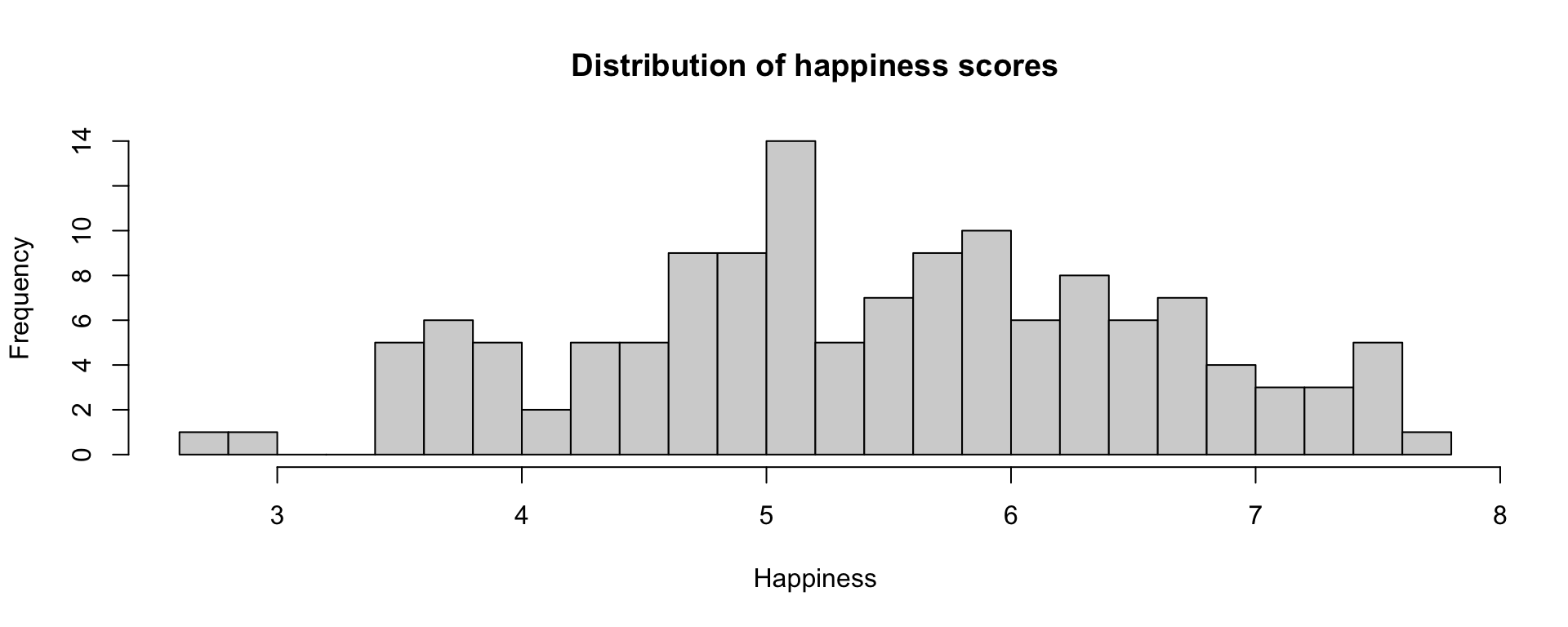
A distribution is a description of the [relative] number of times a variable X will take each of its unique values.
It’s important to remember that the mean of a population (or group) may not represent well some (or any) members of the population.
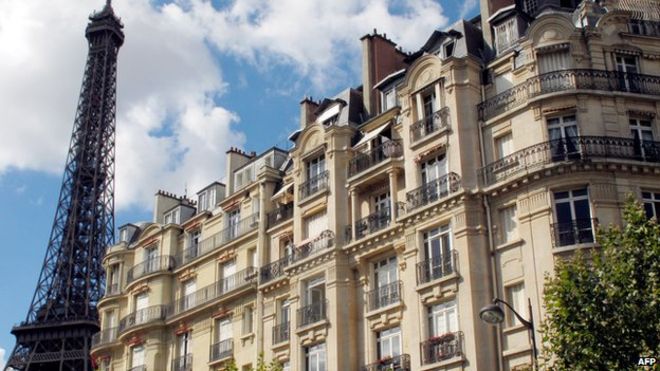
Example: André-François Raffray and the French apartment
Code
world %>% ggplot(aes(x = Happiness)) +
  geom_histogram(fill = "gray") +
  geom_vline(aes(xintercept = mean(Happiness))) +
  geom_vline(aes(xintercept = median(Happiness))) +
  geom_label(aes(x = mean(Happiness), y = maxFreq(Happiness)),
             label = "mean") +
  geom_label(aes(x = median(Happiness), y = maxFreq(Happiness)*2),
             label = "median") +
  labs(y = "Frequency") +
  theme_bw()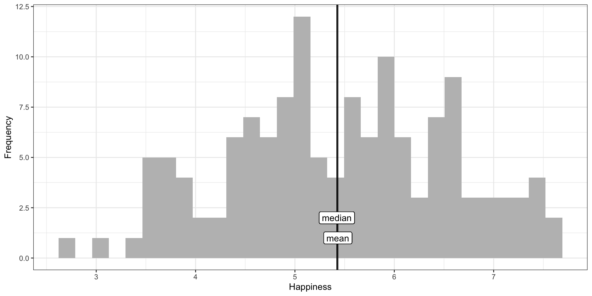
In a normal distribution, the mean, median, and mode are all relatively equal.
Code
world %>% ggplot(aes(x = Corruption)) +
  geom_histogram(fill = "gray") +
  geom_vline(aes(xintercept = mean(Corruption, na.rm=T))) +
  geom_vline(aes(xintercept = median(Corruption, na.rm=T))) +
  geom_label(aes(x = mean(Corruption, na.rm=T), y = maxFreq(Corruption)), label = "mean") +
  geom_label(aes(x = median(Corruption, na.rm=T), y = maxFreq(Corruption)*2), label = "median") +
  labs(y = "Frequency") +
  theme_bw()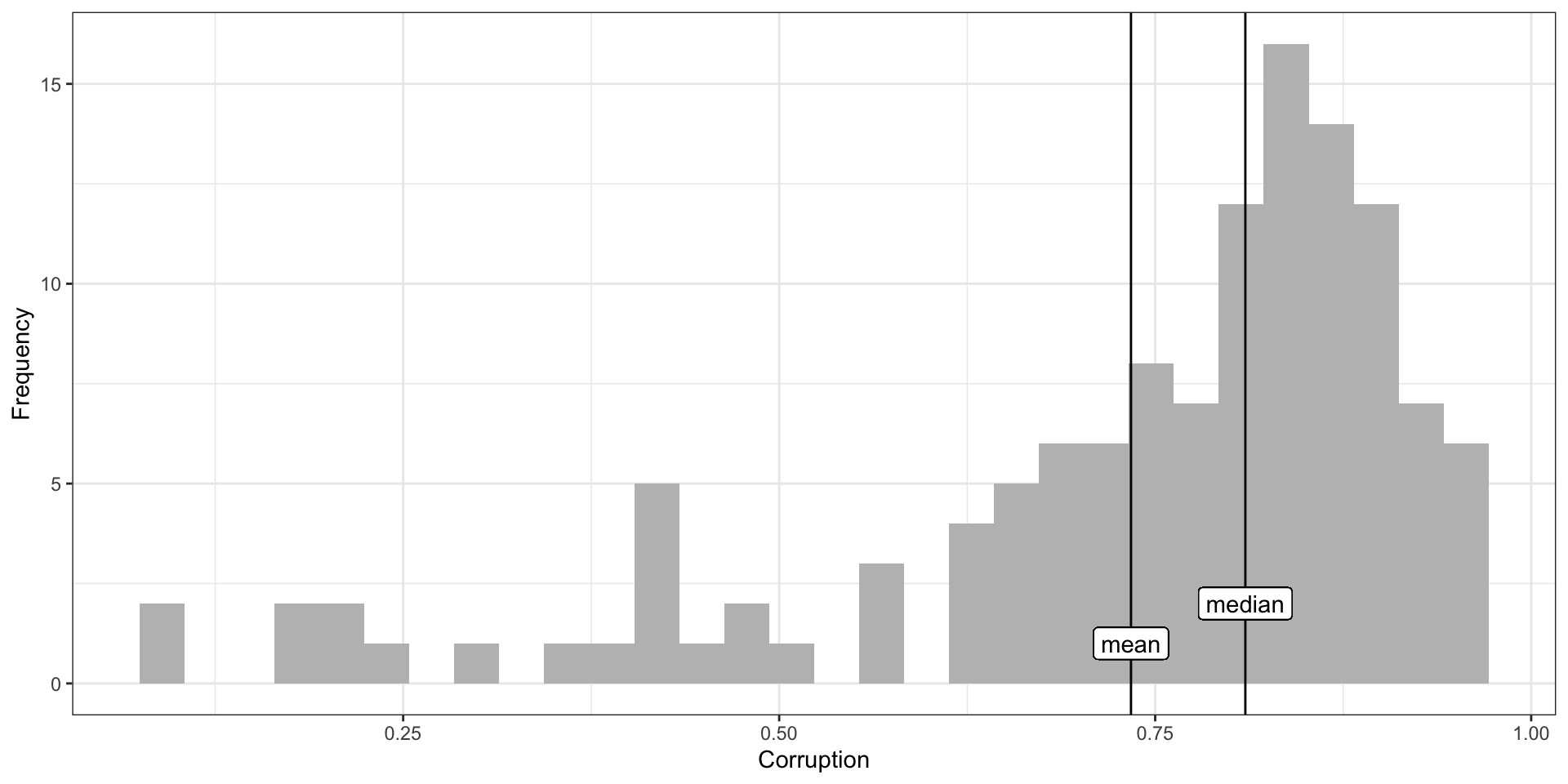
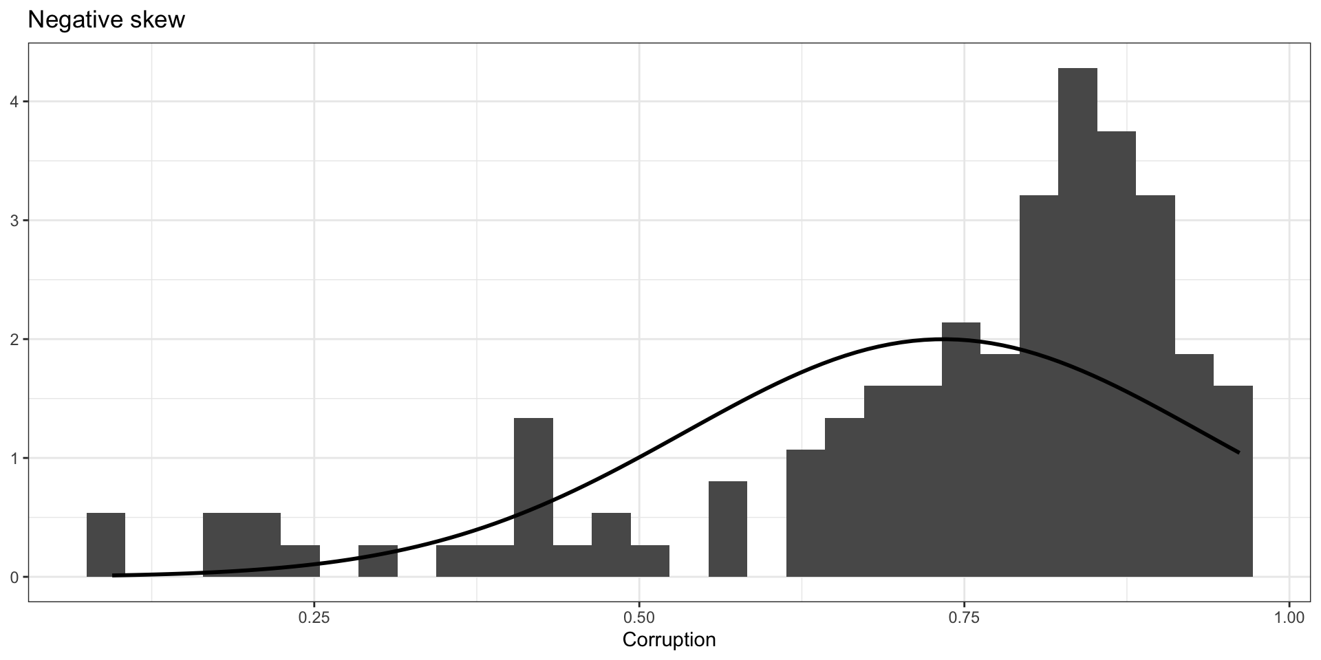
In a skewed distribution, both the mean and median get pulled away from the mode. The mean is pulled further.
Code
world %>% ggplot(aes(x = Corruption)) +
  geom_histogram(fill = "gray") +
  geom_vline(aes(xintercept = median(Corruption, na.rm=T))) +
  geom_label(aes(x = median(Corruption, na.rm=T),
                 y = maxFreq(Corruption)*2),
             label = "median") +
  geom_vline(aes(xintercept = quantile(Corruption,
                                       probs = .25,
                                       na.rm=T)),
             color = "blue") +
  geom_vline(aes(xintercept = quantile(Corruption,
                                       probs = .75,
                                       na.rm=T)),
             color = "blue") +
  geom_label(aes(x = quantile(Corruption,
                              probs = .25,
                              na.rm=T),
                 y = maxFreq(Corruption)*3,
             label = "lower IQR"),
             color = "blue") +
  geom_label(aes(x = quantile(Corruption,
                              probs = .75,
                              na.rm=T),
                 y = maxFreq(Corruption)*4,
             label = "upper IQR"),
             color = "blue") +
  labs(y = "Count") +
  theme_bw()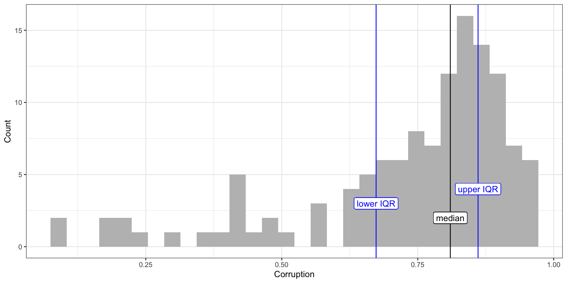
Code
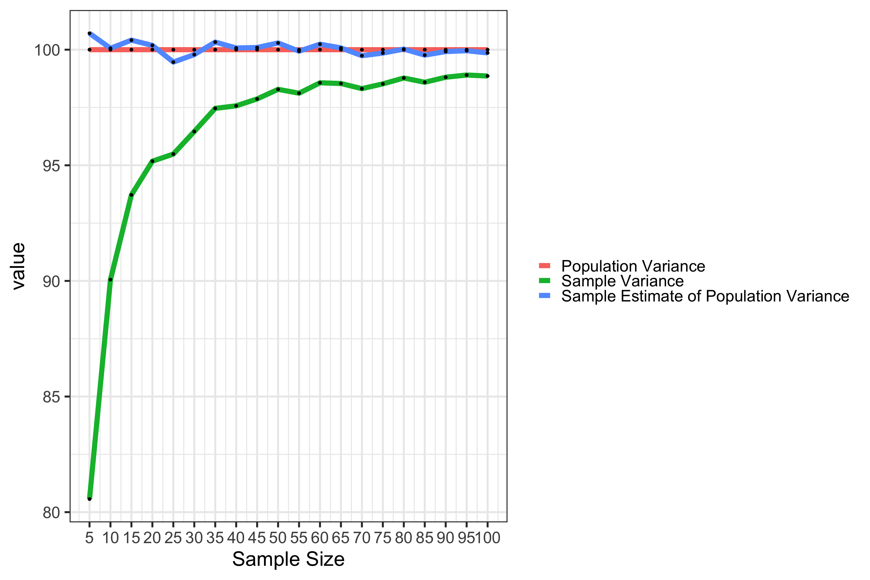
# this is the code that simulates the bias of the variance estimator

# in this simulation, we draw from a known population distribution with
# standard deviation 10.
# for each sample, we calculate the variance using both the population
# formula (dividing by N) and the sample formula (dividing by N-1)

# we repeat this process 10,000 times for each sample size

# for each sample size, we calculate the average estimate of the variance
# using each formula

# this is compared to 100, the true known population variance

set.seed(100917) #so every time I run this, I gets same random draws

# custom function to estimate variance using population formula
sample_var = function(x){
  mx = mean(x, na.rm=T)
  deviations = x-mx
  sq_dev = deviations^2
  ss = sum(sq_dev)
  nx = length(!is.na(x)) #how many not missing
  sample_var = ss/nx
}
#number of samples
draws = 10000
#which sample sizes to test
sample_sizes = seq(from = 5, to = 100, by = 5) # creates c(5, 10, 15, 20, ..., 90, 95, 100)
#data frame to store simulations
var_estimates = data.frame(size = sample_sizes, sample = NA, estimate = NA)

for(i in sample_sizes){ # loop through sample sizes. In each loop, i takes on the next value in the sample_sizes vector
  sample_est = numeric(length = draws) #create empty vector
  estimate = numeric(length = draws) # create empty vector
  for(j in 1:draws){ # loop through draws. In each loop, j takes on new integer
    sample = rnorm(n = i, mean = 1000, sd = 10) # randomly draw sample from pop with variance 100
    sample_est[j] = sample_var(sample) # calculate variance using population formula
    estimate[j] = var(sample) # calculate variance using sample formula
  }
  row = which(var_estimates$size == i) #which row in data frame does this belong to?
  var_estimates$sample[row] = mean(sample_est) # average of variance estimates (using pop) across draws
  var_estimates$estimate[row] = mean(estimate) # average of variances (using sample) across draws
}

var_estimates %>%
  mutate(population = 100) %>% #add population variable
  pivot_longer(cols = c(sample, estimate, population)) %>% # long-form
  mutate(name = factor(name, #lovely labels
                      levels = c("population","sample","estimate"),
                      labels = c("Population Variance",
                                 "Sample Variance",
                                 "Sample Estimate of Population Variance"))) %>%
  ggplot(aes(x = size, y = value)) + # plot, define x and y varibles
  geom_line(aes(color = name), size = 3) + # draw line from each point
  scale_x_continuous("Sample Size", breaks = sample_sizes) + # label x axis
  scale_color_discrete("")+ # no label for color legend
  geom_point() + # add points
  theme_bw(base_size = 25) # nice theme, big font