Describing Data II

Announcements

• Homework 1 due in < two weeks

• Measure yourself for an in-class demo today tinyurl.com/uwn463vj

  • height (inches)
  • length of right forearm (inches)

Population variability

Sums of squares \[ \small SS = \Sigma(X_i-\bar{X})^2 \]

Variance \[ \small \sigma^2 = \frac{\Sigma(X_i-\bar{X})^2}{N} = \frac{SS}{N} \]

Standard deviation \[ \scriptsize \sigma = \sqrt{\frac{\Sigma(X_i-\bar{X})^2}{N}}= \sqrt{\frac{SS}{N}} = \sqrt{\sigma^2} \]

Sample variability

Sums of squares \[ \small SS = \Sigma(X_i-\bar{X})^2 \]

Variance \[ \small \hat{\sigma}^2 = s^2 = \frac{\Sigma(X_i-\bar{X})^2}{N-1} = \frac{SS}{N-1} \] Standard deviation \[ \scriptsize \hat{\sigma} = s = \sqrt{\frac{\Sigma(X_i-\bar{X})^2}{N-1}}= \sqrt{\frac{SS}{N-1}} = \sqrt{s^2} \]

Bi-variate descriptives

Covariation

“Sum of the cross-products”

Population

\[SP_{XY} =\Sigma(X_i−\mu_X)(Y_i−\mu_Y)\] ### Sample

\[ SP_{XY} =\Sigma(X_i−\bar{X})(Y_i−\bar{Y})\]

What does a large, positive SP indicate? A positive relationship, same sign

What does a large, negatve SP indicate? A negative relationship, different sign

What does SP close to 0 indicate? No relationship

Covariance

Sort of like the variance of two variables

Population

\[\sigma_{XY} =\frac{\Sigma(X_i−\mu_X)(Y_i−\mu_Y)}{N}\]

Sample

\[s_{XY} = cov_{XY} =\frac{\Sigma(X_i−\bar{X})(Y_i−\bar{Y})}{N-1}\]

Covariance table

\[\Large \mathbf{K_{XX}} = \left[\begin{array} {rrr} \sigma^2_X & cov_{XY} & cov_{XZ} \\ cov_{YX} & \sigma^2_Y & cov_{YZ} \\ cov_{ZX} & cov_{ZY} & \sigma^2_Z \end{array}\right]\]

Point out that \(cov_{xy}\) is the same as \(cov_{yx}\)

Write on board:

\(cov_{xy} = 126.5\) \(cov_{xz} = 5.2\)

Which variable, Y or Z, does X have greater relationship with? Can’t know because you don’t know what units they’re measured in!

Correlation

• Measure of association

• How much two variables are linearly related

• -1 to 1

• Sign indicates direction of relationship

• Invariant to changes in mean or scaling

Correlation

Pearson product moment correlation

Population

\[\rho_{XY} = \frac{\Sigma z_Xz_Y}{N} = \frac{SP}{\sqrt{SS_X}\sqrt{SS_Y}} = \frac{\sigma_{XY}}{\sigma_X \sigma_Y}\]

Sample \[r_{XY} = \frac{\Sigma z_Xz_Y}{n-1} = \frac{SP}{\sqrt{SS_X}\sqrt{SS_Y}} = \frac{s_{XY}}{s_X s_Y}\]

Why is it called the Pearson Product Moment correlation? Pearson = Karl Pearson Product = multiply Moment = variance is the second moment of a distribution

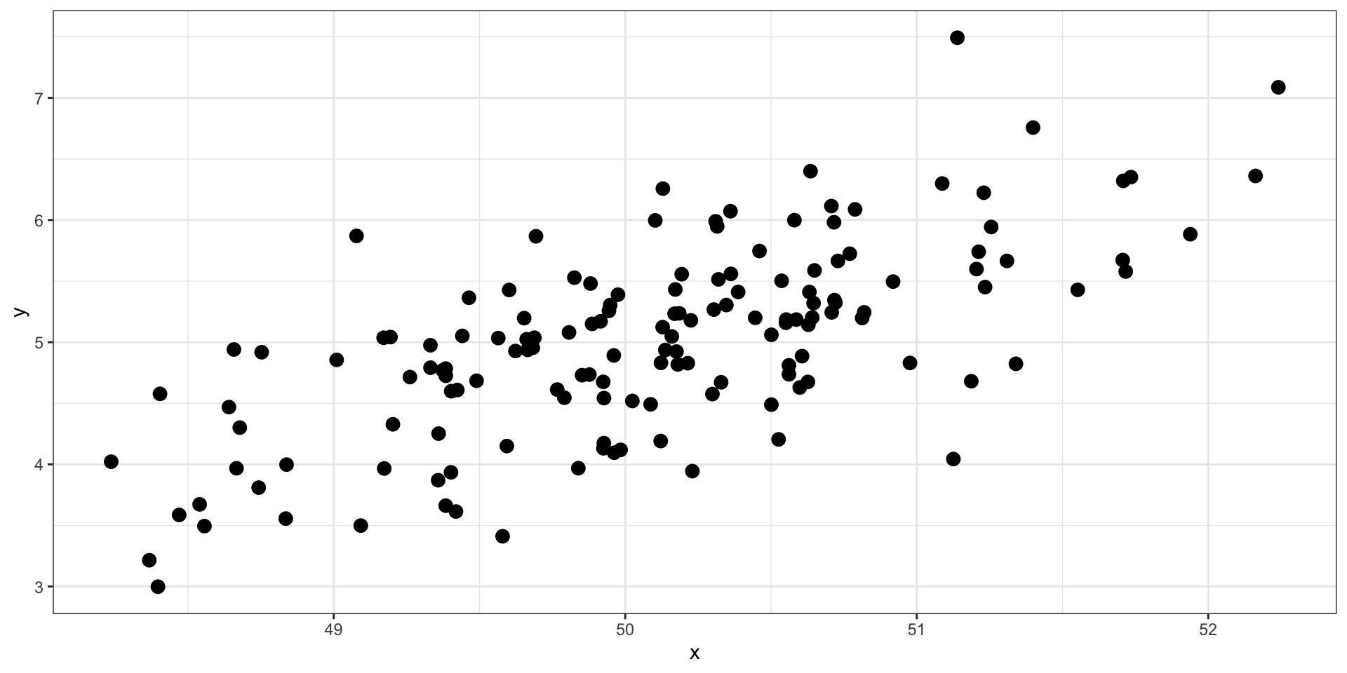
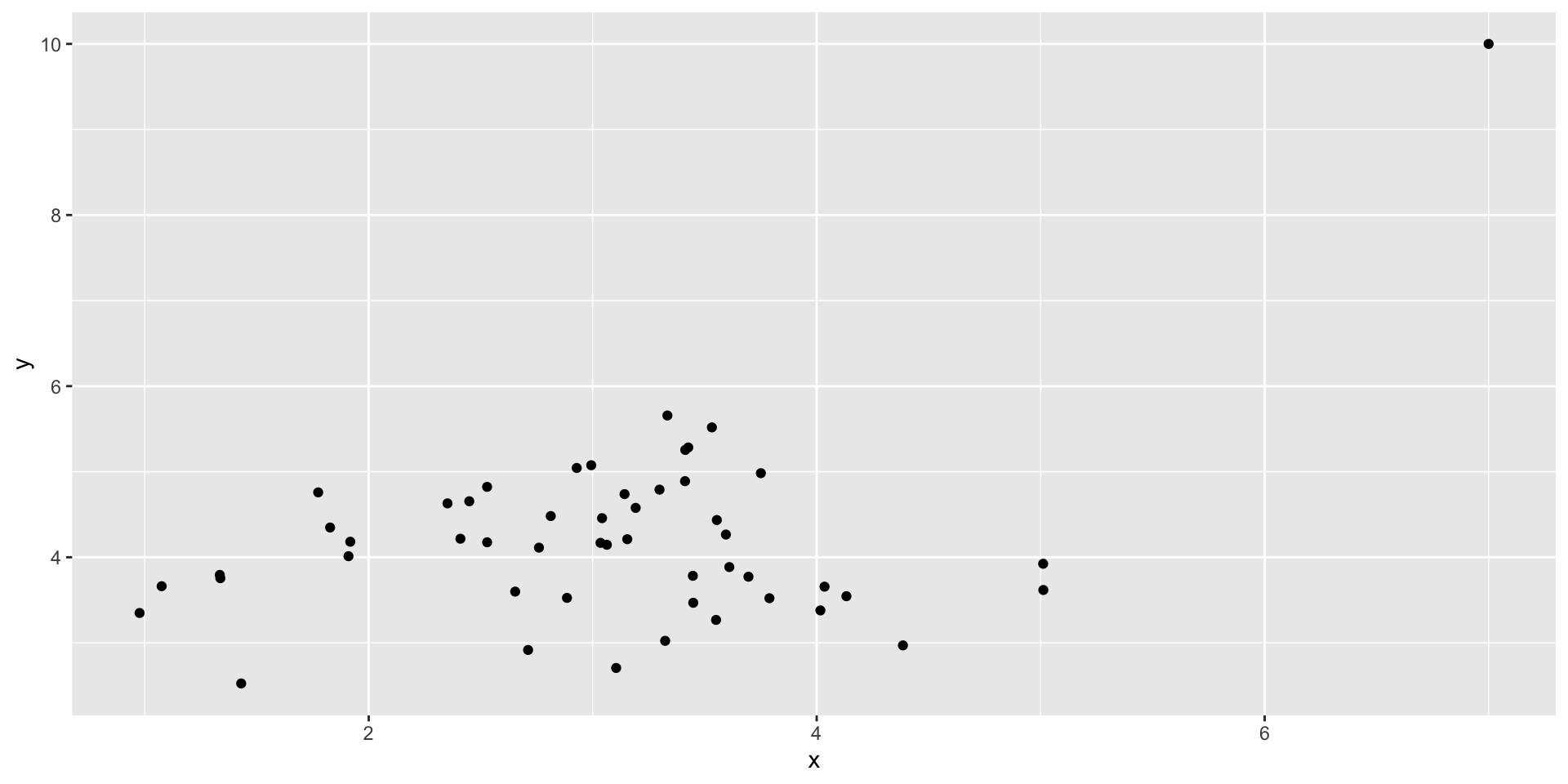
set.seed(101019) # so we all get the same random numbers
mu = c(50, 5) # means of two variables (MX = 50, MY = 5)
Sigma = matrix(c(.8, .5, .5, .7), ncol =2) #diagonals are reliabilites, off-diagonals are correlations
data = mvrnorm(n = 150, mu = mu, Sigma = Sigma)
data = as.data.frame(data)
colnames(data) = c("x", "y")
data %>% ggplot(aes(x = x, y = y)) + geom_point(size = 3) + theme_bw()

What is the correlation between these two variables?

Correlation = 0.68

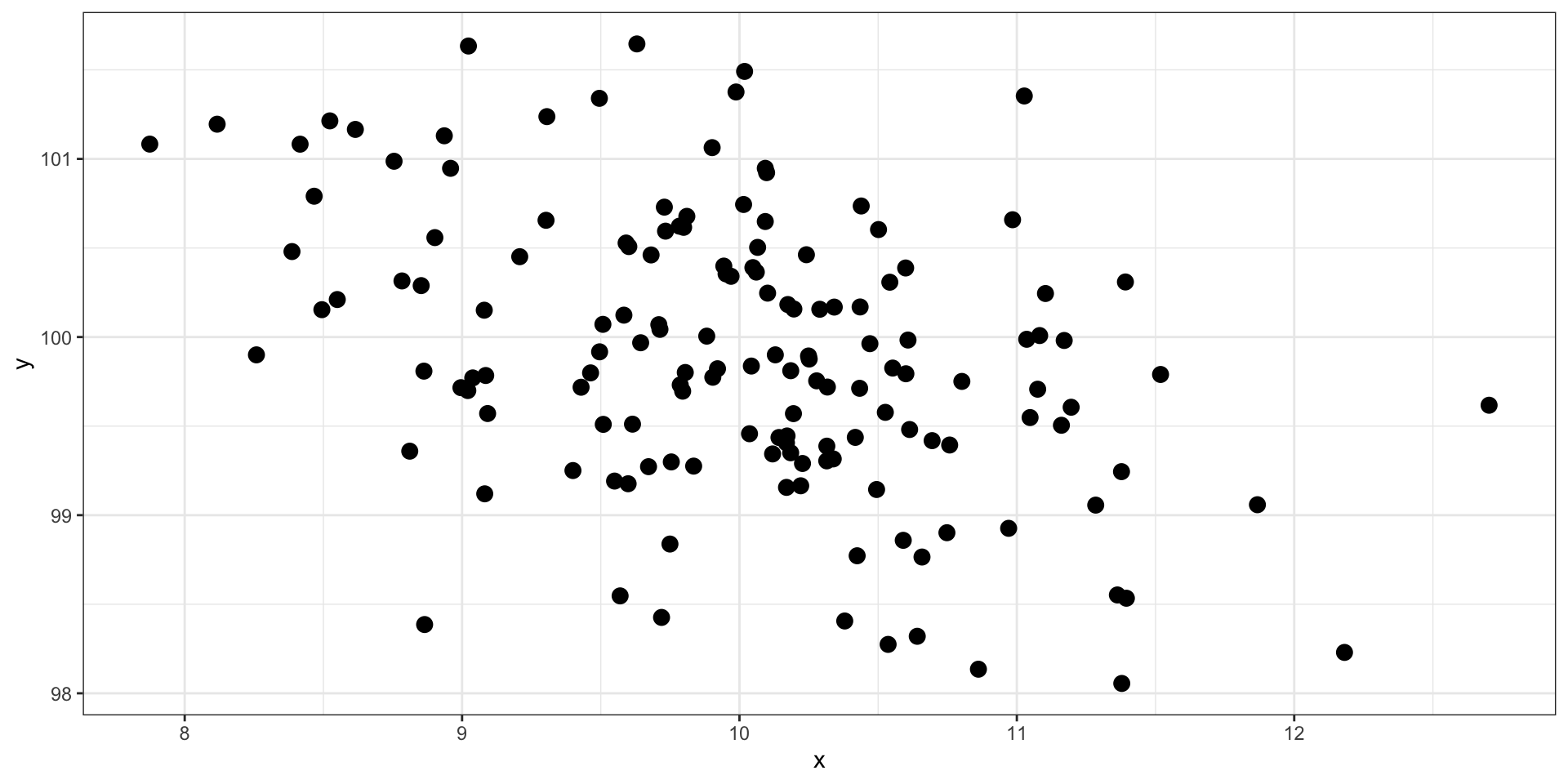
set.seed(101019) # so we all get the same random numbers
mu = c(10, 100)
Sigma = matrix(c(.8, -.3, -.3, .7), ncol =2) #diagonals are reliabilites, off-diagonals are correlations
data = mvrnorm(n = 150, mu = mu, Sigma = Sigma)
data = as.data.frame(data)
colnames(data) = c("x", "y")

data %>% ggplot(aes(x = x, y = y)) + geom_point(size = 3) + theme_bw()

What is the correlation between these two variables?

Correlation = -0.41

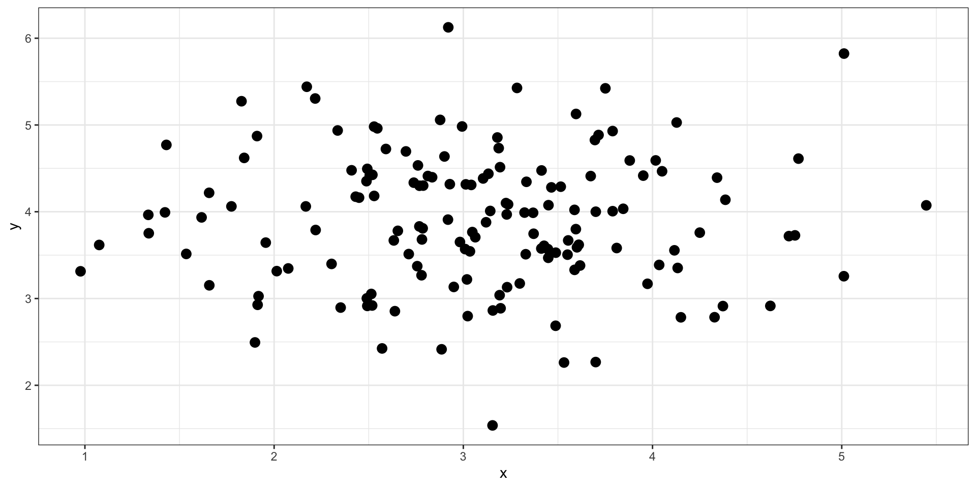
set.seed(101019) # so we all get the same random numbers
mu = c(3, 4)
Sigma = matrix(c(.8, 0, 0, .7), ncol =2) #diagonals are reliabilites, off-diagonals are correlations
data = mvrnorm(n = 150, mu = mu, Sigma = Sigma)
data = as.data.frame(data)
colnames(data) = c("x", "y")
data %>% ggplot(aes(x = x, y = y)) + geom_point(size = 3) + theme_bw()

What is the correlation between these two variables?

Correlation = 0

Effect size

• Recall that z-scores allow us to compare across units of measure; the products of standardized scores are themselves standardized.

• The correlation coefficient is a standardized effect size which can be used communicate the strength of a relationship.

• Correlations can be compared across studies, measures, constructs, time.

• Example: the correlation between age and height among children is \(r = .70\). The correlation between self- and other-ratings of extraversion is \(r = .25\).

What is a large correlation?

- Cohen (1988): .1 (small), .3 (medium), .5 (large)

• Often forgot: Cohen said only to use them when you had nothing else to go on, and has since regretted even suggesting benchmarks to begin with. |

• Rosenthal & Rubin (1982): life and death (the Binomial Effect Size Display)

  • treatment success rate \(= .50 + .5(r)\) and the control success rate \(= .50 - .5(r)\).

What is a large correlation?

• \(r^2\): Proportion of variance “explained”
  • Ozer & Funder (2019) claim this is misleading and nonsensical
  • Fisher (2019) suggests this particular argument is non-scientific (follow up here and then here)

Funder & Ozer (2019)

• Effect sizes are often mis-interpreted. How?

• What can fix this?

• Pitfalls of small effects and large effects

• Recommendations?

“benchmarks” lack context and are arbitrary

fix: - better benchmarks - compare with classic studies or other literature or all literature - compare with non-psychological phenomenon - explain in terms of consequences - BESD - long-run consequences

Recommendations - Report effect sizes - Use large samples – remember bias? - Report effect sizes in context - Stop using empty terminology - Revise guildelines

What affects correlations?

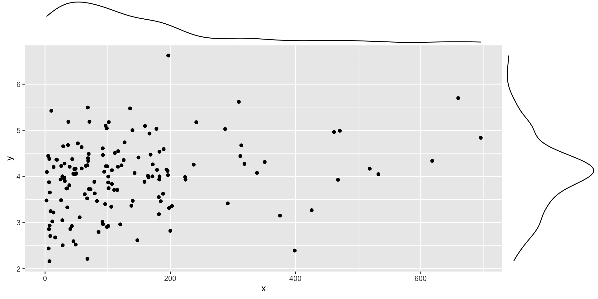
It’s not enough to calculate a correlation between two variables. You should always look at a figure of the data to make sure the number accurately describes the relationship. Correlations can be easily fooled by qualities of your data, like:

• Skewed distributions

• Outliers

• Restriction of range

• Nonlinearity

Skewed distributions

set.seed(101019) # so we all get the same random numbers
mu = c(3, 4)
Sigma = matrix(c(.8, .2, .2, .7), ncol =2) #diagonals are reliabilites, off-diagonals are correlations
data = mvrnorm(n = 150, mu = mu, Sigma = Sigma)
data = as.data.frame(data)
colnames(data) = c("x", "y")
data$x = data$x^4

p = data %>% ggplot(aes(x=x, y=y)) + geom_point()
ggMarginal(p, type = "density")

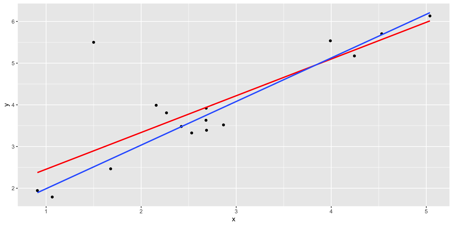
Outliers

set.seed(101019) # so we all get the same random numbers
mu = c(3, 4)
Sigma = matrix(c(.8, 0, 0, .7), ncol =2) #diagonals are reliabilites, off-diagonals are correlations
data = mvrnorm(n = 50, mu = mu, Sigma = Sigma)
data = as.data.frame(data)
colnames(data) = c("x", "y")
data[51, ] = c(7, 10)
data %>% ggplot(aes(x=x, y=y)) + geom_point() 

Outliers

data %>% ggplot(aes(x=x, y=y)) + geom_point() + geom_smooth(method = "lm", se = FALSE, color = "red") + geom_smooth(data = data[-51,], method = "lm", se = FALSE)

Outliers

set.seed(101019) # so we all get the same random numbers
mu = c(3, 4)
n = 15
Sigma = matrix(c(.9, .8, .8, .9), ncol =2) #diagonals are reliabilites, off-diagonals are correlations
data = mvrnorm(n = n, mu = mu, Sigma = Sigma)
data = as.data.frame(data)
colnames(data) = c("x", "y")
data[n+1, ] = c(1.5, 5.5)

data %>% ggplot(aes(x=x, y=y)) + geom_point() + geom_smooth(method = "lm", se = FALSE, color = "red") + geom_smooth(data = data[-c(n+1),], method = "lm", se = FALSE)

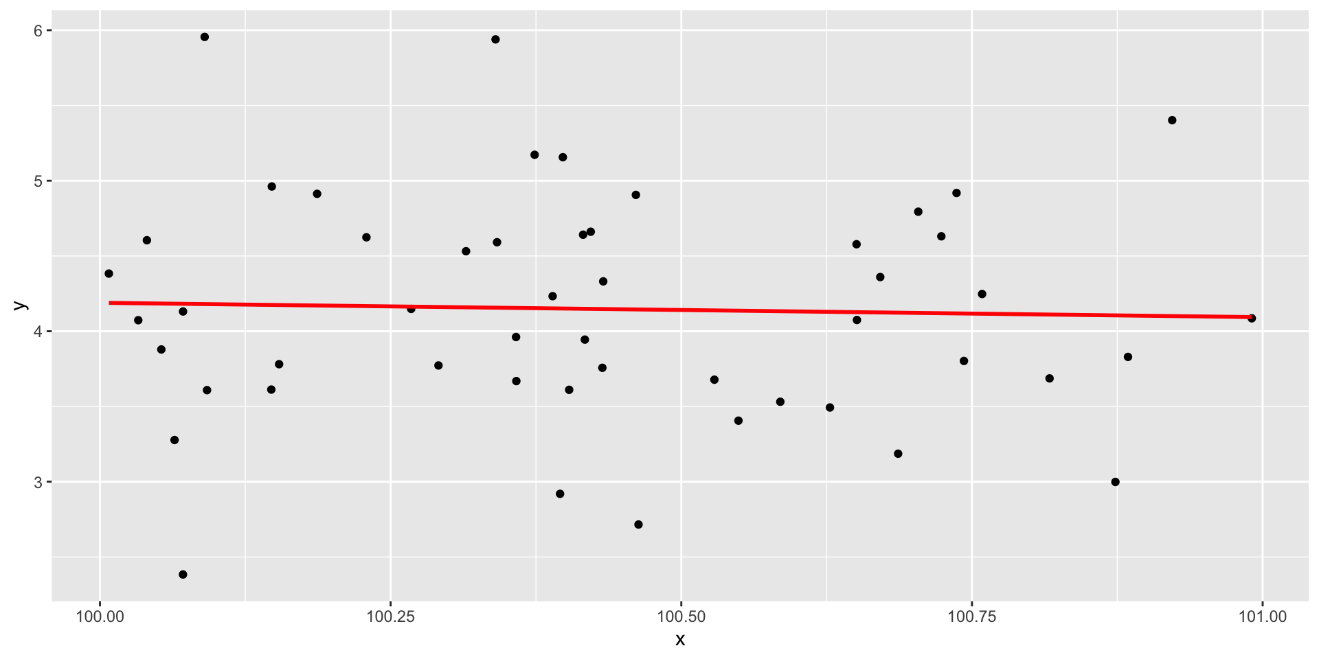
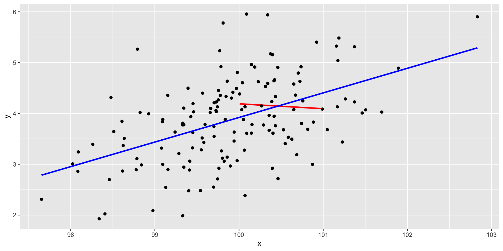
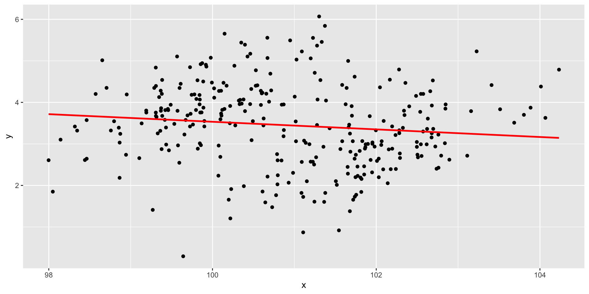
Restriction of range

set.seed(1010191) # so we all get the same random numbers
mu = c(100, 4)
Sigma = matrix(c(.7, .4, 4, .75), ncol = 2) #diagonals are reliabilites, off-diagonals are correlations
data = mvrnorm(n = 150, mu = mu, Sigma = Sigma)
data = as.data.frame(data)
colnames(data) = c("x", "y")
real_data = data
data = filter(data, x >100 & x < 101)

data %>% ggplot(aes(x=x, y=y)) + geom_point() + geom_smooth(method = "lm", se = FALSE, color = "red")

What if I told you there were scores on X could range from 97 to 103?

Restriction of range

data %>% ggplot(aes(x=x, y=y)) + geom_point() + geom_smooth(method = "lm", se = FALSE, color = "red") + geom_point(data = real_data) + geom_smooth(method = "lm", se = FALSE, data = real_data, color = "blue")

Can you think of example where this might occur in psychology? My idea: that many psychology studies only look at undergraduates (restricted age, restricted education) – can’t use these as predictors or covariates

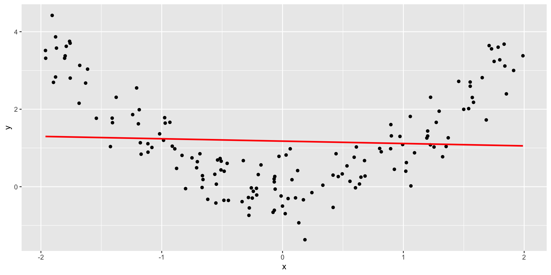
Nonlinearity

x = runif(n = 150, min = -2, max = 2)
y = x^2 +rnorm(n = 150, sd = .5)
data = data.frame(x,y)

data %>% ggplot(aes(x=x, y=y)) + geom_point() + geom_smooth(method = "lm", se = FALSE, color = "red")

It’s not always apparent

Sometimes issues that affect correlations won’t appear in your graph, but you still need to know how to look for them.

• Low reliability

• Content overlap

• Multiple groups

Reliability

\[r_{xy} = \rho_{xy}\sqrt{r_{xx}r_{yy}}\]

Meaning that our estimate of the population correlation coefficient is attenuated in proportion to reduction in reliability.

If you have a bad measure of X or Y, you should expect a lower estimate of \(\rho\).

Content overlap

If your Operation Y of Construct B includes items (or tasks or manipulations) that could also be influenced by Constrct A, then the correlation between X and Y will be inflated.

• Example: SAT scores and IQ tests

• Example: Depression and number of hours sleeping

• Which kind of validity is this associated with?

In-class demo

Add your height (in inches), forearm length (in inches), and gender to this spreadsheet: tinyurl.com/uwn463vj

Correlation in Pearson & Lee (1903) is about .627.

Calculate correlation in class

• Why does Pearson find smaller correlation? Students generate ideas

Show disaggregated correlation by gender (no graph)

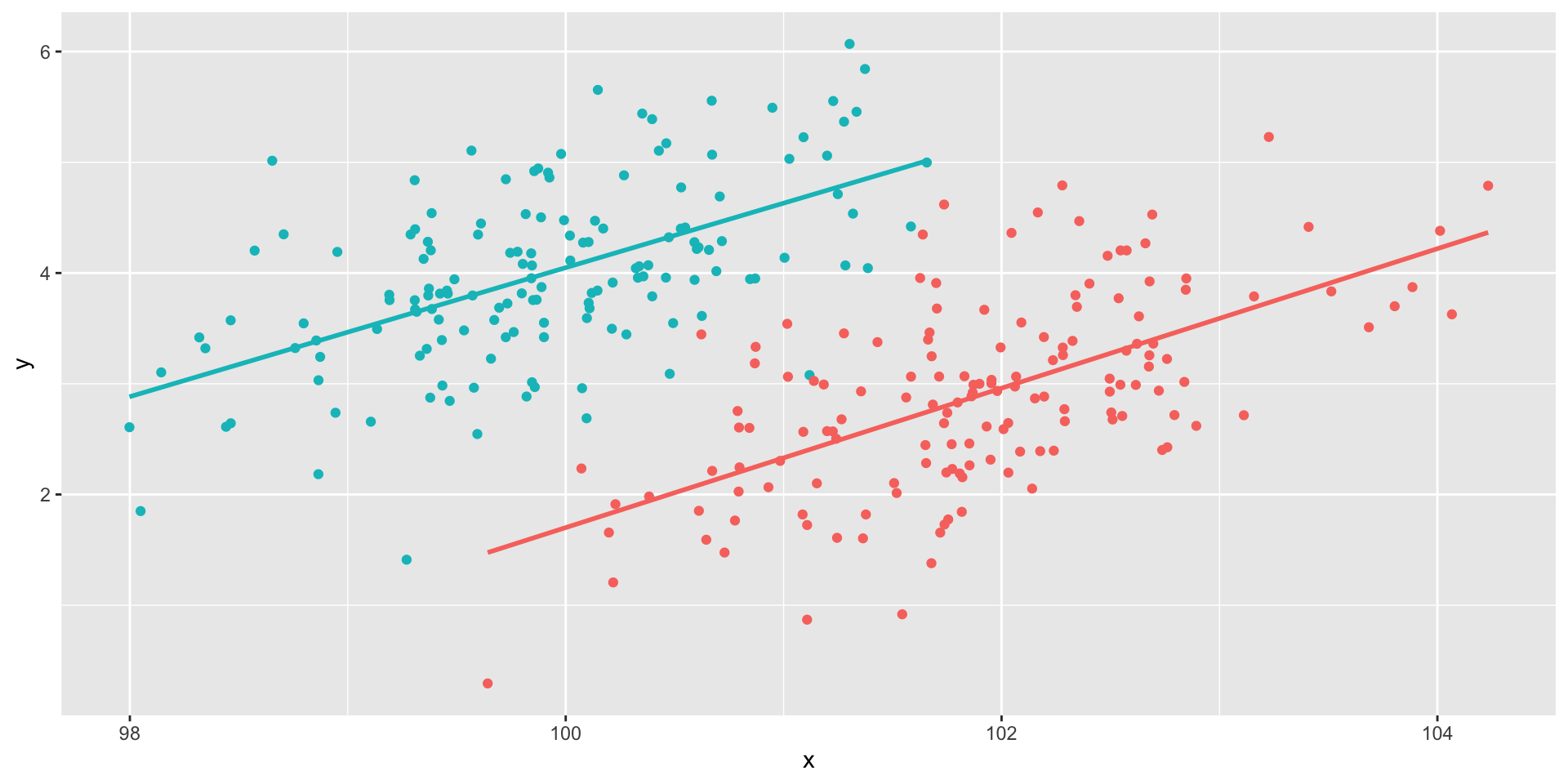
Multiple groups

set.seed(101019) # so we all get the same random numbers
m_mu = c(100, 4)
m_Sigma = matrix(c(.7, .4, 4, .75), ncol = 2) #diagonals are reliabilites, off-diagonals are correlations
m_data = mvrnorm(n = 150, mu = m_mu, Sigma = m_Sigma)
m_data = as.data.frame(m_data)
colnames(m_data) = c("x", "y")

f_mu = c(102, 3)
f_Sigma = matrix(c(.7, .4, 4, .75), ncol = 2) #diagonals are reliabilites, off-diagonals are correlations
f_data = mvrnorm(n = 150, mu = f_mu, Sigma = f_Sigma)
f_data = as.data.frame(f_data)
colnames(f_data) = c("x", "y")

m_data$gender = "male"
f_data$gender = "female"

data = rbind(m_data, f_data)

data %>% ggplot(aes(x=x, y=y)) + geom_point() + geom_smooth(method = "lm", se = FALSE, color = "red")

Multiple groups

data %>% ggplot(aes(x=x, y=y, color = gender)) + geom_point() + geom_smooth(method = "lm", se = FALSE) + guides(color = "none")

Special cases of the Pearson correlation

• Spearman correlation coefficient
  • Applies when both X and Y are ranks (ordinal data) instead of continuous
  • Denoted \(\rho\) by your textbook, although I prefer to save Greek letters for population parameters.
• Point-biserial correlation coefficient
  • Applies when Y is binary.
• Phi ( \(\phi\) ) coefficient
  • Both X and Y are dichotomous.

Do the special cases matter?

For Spearman, you’ll get a different answer.

x = rnorm(n = 10); y = rnorm(n = 10) #randomly generate 10 numbers from normal distribution

Here are two ways to analyze these data

head(cbind(x,y))

              x          y
[1,] -0.6682733 -0.3940594
[2,] -1.7517951  0.9581278
[3,]  0.6142317  0.8819954
[4,] -0.9365643 -1.7716136
[5,] -2.1505726 -1.4557637
[6,] -0.3593537 -1.2175787

cor(x,y, method = "pearson")

[1] 0.2702894

head(cbind(x,y, rank(x), rank(y)))

              x          y     
[1,] -0.6682733 -0.3940594  5 7
[2,] -1.7517951  0.9581278  2 9
[3,]  0.6142317  0.8819954 10 8
[4,] -0.9365643 -1.7716136  4 3
[5,] -2.1505726 -1.4557637  1 4
[6,] -0.3593537 -1.2175787  7 6

cor(x,y, method = "spearman")

[1] 0.3454545

Do the special cases matter?

If your data are naturally binary, no difference between Pearson and point-biserial.

x = rnorm(n = 10); y = rbinom(n = 10, size = 1, prob = .3)
head(cbind(x,y))

               x y
[1,] -0.48974849 1
[2,] -2.53667101 0
[3,]  0.03521883 1
[4,]  0.03043436 0
[5,] -0.27043857 0
[6,] -0.55228283 1

Here are two ways to analyze these data

cor(x,y, method = "pearson")

[1] 0.1079188

ltm::biserial.cor(x,y)

[1] -0.1079188

Do the special cases matter?

If artificially dichotomize data, there can be big differences. This is bad.

x = rnorm(n = 10); y = rnorm(n = 10)

Here are two ways to analyze these data

head(cbind(x,y))

               x          y
[1,]  1.27516603 -0.2012149
[2,] -1.55729177  0.2925842
[3,]  0.09364959  0.0821713
[4,]  0.87343693  0.1879078
[5,]  0.74807054  0.3794815
[6,]  0.02831971 -1.2940189

cor(x,y, method = "pearson")

[1] -0.1584301

d_y = ifelse(y < median(y), 0, 1)
head(cbind(x,y, d_y))

               x          y d_y
[1,]  1.27516603 -0.2012149   0
[2,] -1.55729177  0.2925842   1
[3,]  0.09364959  0.0821713   0
[4,]  0.87343693  0.1879078   0
[5,]  0.74807054  0.3794815   1
[6,]  0.02831971 -1.2940189   0

ltm::biserial.cor(x, d_y)

[1] 0.4079477

Don’t use median splits!

Why? * Median spilts can change relationship of observation to center (observation which is higher than mean may be lower than median) * Correlations are based on moments of distribution (mean and variance), and rescaling to median violates this assumption

Special cases of the Pearson correlation

Why do we have special cases of the correlation?

• Sometimes we get different results

  • If we treat ordinal data like interval/ratio data, our estimate will be incorrect

• Sometimes we get the same result

  • Even when formulas are different

  • Example: Point biserial formula

    • \[r_{pb} = \frac{M_1-M_0}{\sqrt{\frac{1}{n-1}\Sigma(X_i-\bar{X})^2}}\sqrt{\frac{n_1n_0}{n(n-1)}}\]

We don’t have different formulas because the correlation is mathematically different – these formulas were developed when we did things by hand. These formulas are short cuts!

Next time…

Probability!