The binomial distribution is the theoretical probability distribution appropriate when modeling the expected outcome, X, of N trials (or event sequences) that have the following characteristics:
The outcome on every trial is binary
also called a Bernoulli trial
The probability of the target outcome (usually called a “success”) is the same for all N trials
“with replacement” might be necessary
The trials are independent
The number of trials is fixed
If these assumptions hold then X is a binomial random variable representing the expected number of successes over N trials, with expected success on each trial of \(\theta\) .
A common and compact way of stating the same thing is:
\[\large X \sim B(N, \theta)\]
The probability distribution for X is defined by the following probability mass function:
The probability mass function tells us what to expect for any particular X in the sample space.
All theoretical distributions have a mass function (if discrete) or a density function (if continuous). These are the defining equations that tells us the generating process for the behavior of X.
Many texts refer to the probability of success as \(p\) and the probability of not success (or failure) as \(q\):
\[P(X|p, N)= \frac{N!}{X!(N-X)!}p^Xq^{(N-X)}\]
What does the Law of Total Probability require to be true?
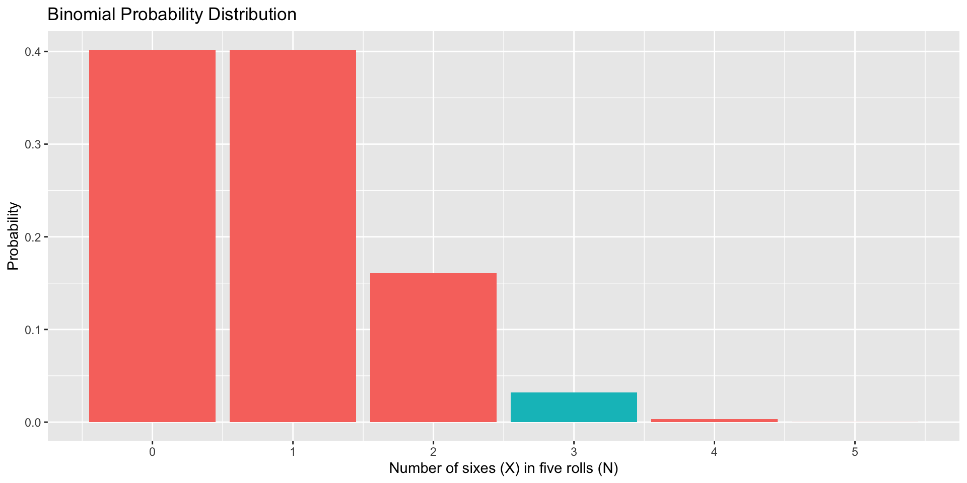
Code
data.frame(num =0:5, p =dbinom(x =0:5, size =5, prob =1/6), three =as.factor(c(0,0,0,1,0,0))) %>%ggplot(aes(x=num, y=p, fill = three)) +geom_bar(stat="identity") +scale_x_continuous("Number of sixes (X) in five rolls (N)", breaks=c(0:5)) +scale_y_continuous("Probability")+guides(fill ="none") +ggtitle("Binomial Probability Distribution")
Every probability distribution has an expected value distribution.
For the binomial distribution:
\[E(X) = N\theta\]
Each probability distribution also has a variance. For the binomial:
\[Var(X) = N\theta(1-\theta)\]
Importantly, this means our mean and variance are related in the binomial distribution, because they both depend on \(\theta\). How are they related?
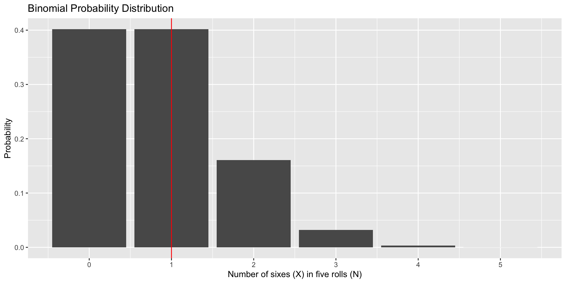
If you have a discrete distribution with a small N, these estimates may not have a sensible meaning.
Later we will use the variance to help us make statements about how confident we are with regard to the location of the mean.
The mean, .835, does not exist in the sample space, and rounding up to 1 and claiming that to be the most typical outcome is not quite right either.
The probability mass (density) function allows us to answer other questions about the sample space that might be more important, or at least realistic.
mass = discrete
density = continuous
I might want to know the value in the sample space at or below which a certain proportion of outcomes fall. This is a percentile or quantile question.
“Most (75%) of five dice rolls yield X or fewer 6’s.”
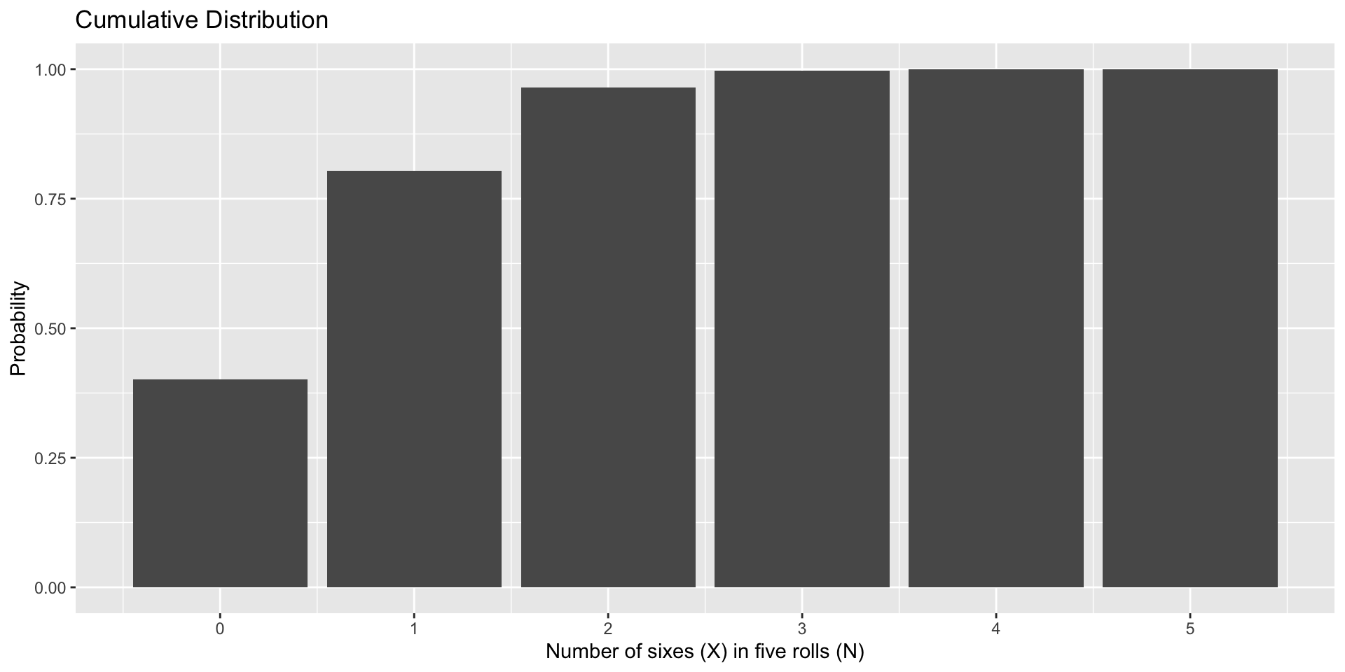
I might want to know the proportion of outcomes in the sample space that fall at or below a particular outcome. This is a cumulative proportion question. - “What percentage of the time will my outcome be less than 3?”
At or below what outcome in the sample space do .75 of the outcomes fall?
What proportion of outcomes in the sample space that fall at or below a given outcome?
In R, we can calculate the cumulative probability (X or lower), using the pbinom function.
# what is probability of rolling two or fewer 6's out of five rolls?pbinom(q =2, size =5, prob =1/6)
[1] 0.9645062
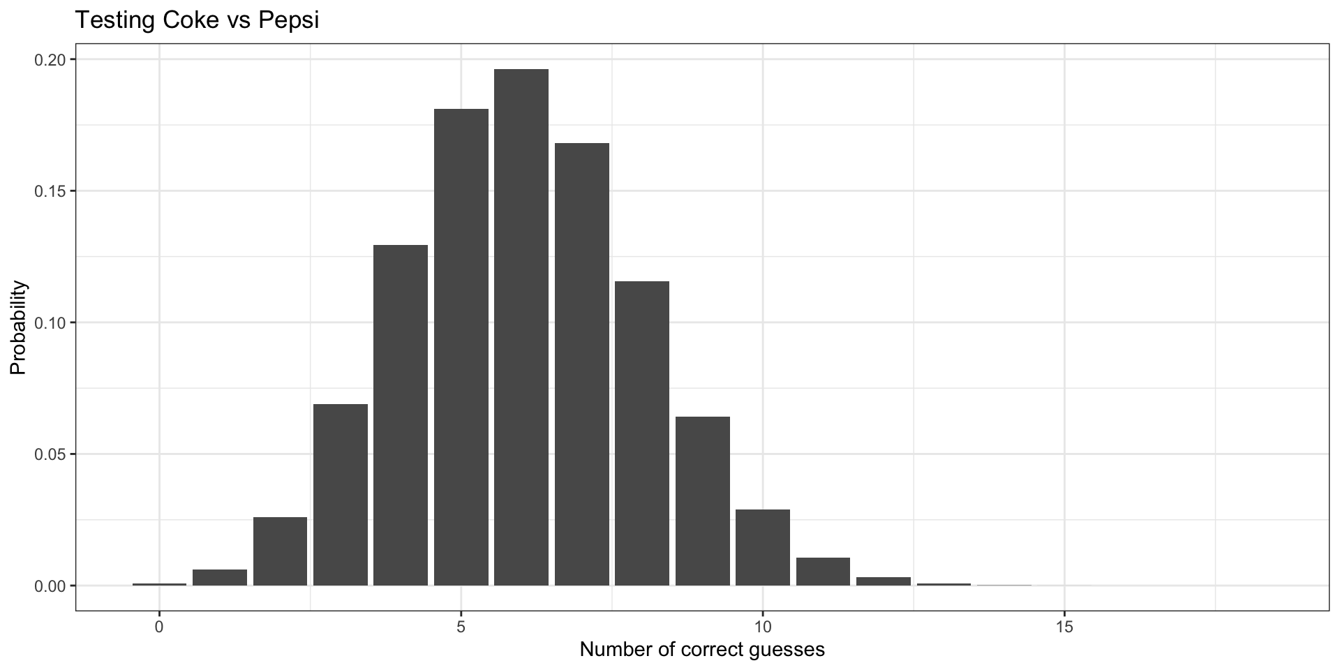
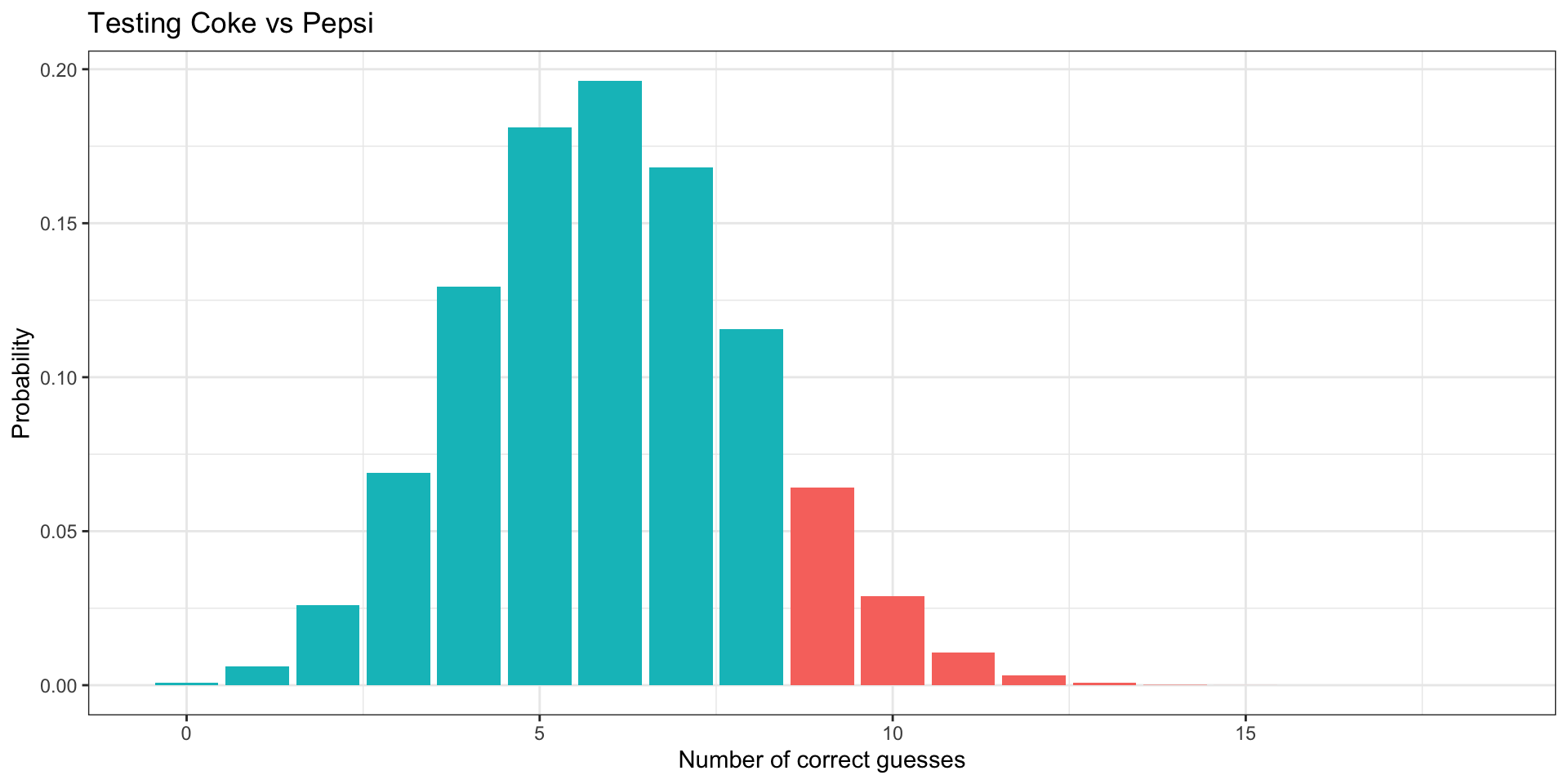
The binomial is of interest beyond describing the behavior of dice and coins.
Many practical outcomes might be best described by a binomial distribution.
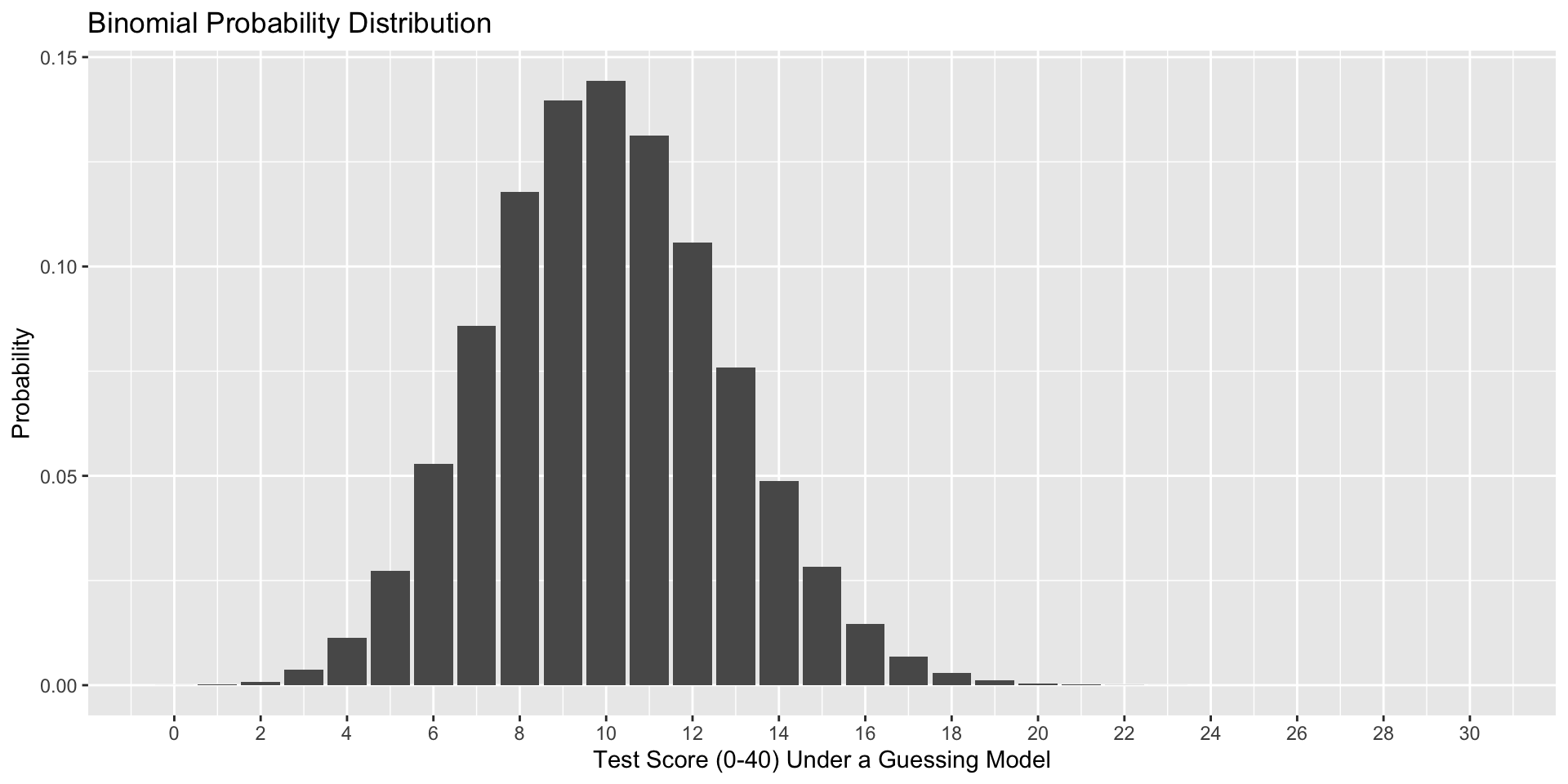
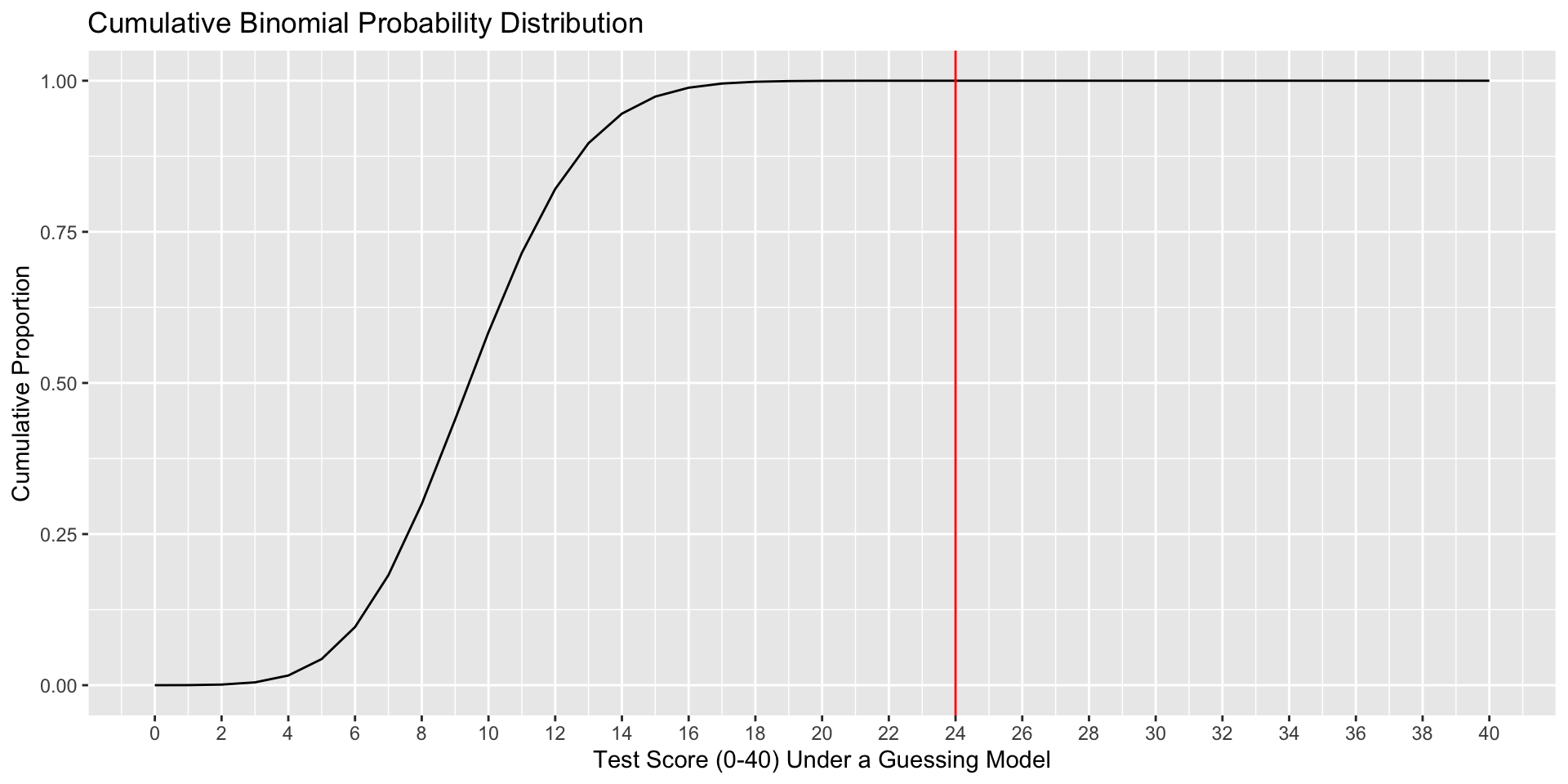
For example, suppose I give a 40-item multiple choice test, with each question having 4 options.
I am worried that students might do well by chance alone. I would not want to pass students in the class if they were just showing up for the exams and guessing for each question.
What are the parameters in the binomial distribution that will help me address this question?
How likely is it that a guesser would score above the threshold (60%) necessary to pass the class by the most minimal standards?
But, what assumptions are we making and what consequences will they have?
The outcome on every trial is binary (also called a Bernoulli trial)
The probability of the target outcome (usually called a “success”) is the same for all N trials (“with replacement” might be necessary)
The trials are independent \(P(A\cap B) = P(A|B)P(B)=P(A)P(B)\)
The number of trials is fixed
We might have viable alternative models:
Geometric distribution: Used if we are interested in the number of trials required for one “success” to occur
“how many times do I start my computer before it fails to start at all?”
We might have viable alternative models:
Negative binomial distribution: Used if we are interested in the number of trials required for a specific number of “successes” to occur
“A child won’t return from trick or treating until they get 5 full-size candy bars. What is the probability that they will have to visit 34 homes to get this?”
We might have viable alternative models:
Poisson distribution: Used when there’s not a fixed number of trials but rather a fixed interval of time.
“What is the expected number of times a solider will be kicked in the head by a horse and die during this one year campaign?”