Make sure your answer shows up in the knitted file.
knit early and often
Homework is for learning, not for testing
Work together
library(tidyverse) #plottinglibrary(ggforce) # for plotting circleslibrary(ggpubr) #prettier figures
Last time…
Normal distributions!
Why is the normal distribution useful?
Follows a specific shape
Defined by 2 parameters
Area under the curve = 1
Law of Total Probability
How likely is any range of values?
Cool, but can we assume our statistics follow a normal distribution? Today… sampling!
To this point, we have assumed that features of the population – the parameters – are known. That is rarely the case.
The major goal that we have in statistical inference is to make confident claims about the population based on a small representation of it, the sample.
Our confidence in the sample as a representation of the population relies on sampling theory.
Terms
Sample: The particular units from a population on which measures are collected (the data).
Population: The complete set of units (e.g., people, countries, etc.) from which a sample is selected.
Sampling method: The procedure used to create a sample.
Ideally we would like to believe that there is nothing special about a sample. Any other sample from the same population should be interchangeable with the one we have in hand. Any sample should be able to “stand for” or be a good proxy for the population.
Interchangeable or representative samples allow us to make confident claims about the population.
Samples are representative to the extent the population is clearly defined and the sample is selected using an appropriate sampling method.
Probability sampling methods maintain a defensible link between a sample and population. This link is based on statistical theory and rules of probability.
Nonprobability sampling methods provide only a weak link between a sample and population. This link is based on appeals to common sense and reason. Maybe only blind faith.
Despite the clear distinction, it is not unusual for researchers to use a nonprobability sampling method and then draw inferences in a way that implies a strong link from the sample to some population.
Probability sampling methods have the following simple features:
Define the population so that all population units can be identified (i.e., become candidates for selection).
Select a sample from among those units using a random selection method.
Common random sampling methods:
Simple random sampling: Each of the units in the population has an equal chance of being selected.
Stratified random sampling: Identify nonoverlapping strata and carry out simple random sampling within each strata.
Cluster random sampling: Divide the population into nonoverlapping clusters. Randomly select clusters and use all of the units within the selected clusters.
Multistage random sampling: A combination of the other random sampling methods (stratified random sampling within clusters).
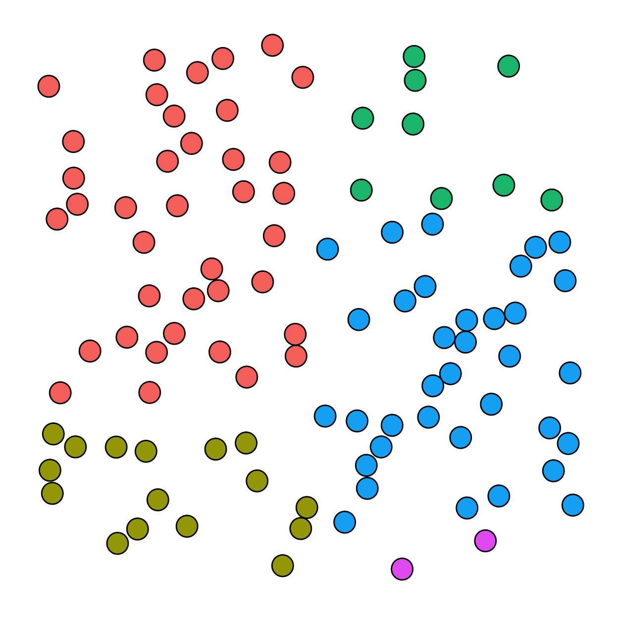
Simple random sampling
In simple random sampling, each object would have an equal probability of being selected (1/100). For simple random sampling, any object characteristics (e.g., color) are irrelevant.
Stratified random sampling
In stratified random sampling, the objects are first categorized into strata (e.g., color) and random sampling occurs within strata. The probability of being selected depends on the size of the strata (1/38 in the red strata; 1/2 in the purple strata).
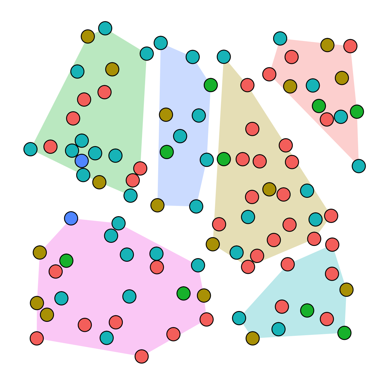
Cluster Random Sampling
In cluster random sampling, clusters of units are selected at random and then all of the units within the chosen clusters are part of the sample. The probability of a particular unit being sampled is a function of the number of clusters.
No matter what probability method we use, we know the probability that a unit from the population will be selected. This allows us to determine the sampling error so that we can know how well the sample represents the population.
Any sample will be off the mark in how well it captures the important features of the population. With probability sampling methods we can estimate how far off the mark we are likely to be.
Nonprobability sampling methods
Nonprobability sampling methods select the sample on some basis other than a random process. As a consequence, how well the sample represents the population can be difficult to know and the argument depends on common sense and appeals to reason. These methods include:
Convenience sampling
Purposive sampling
Modal instance sampling
Expert sampling
Quota sampling
Heterogeneity sampling
Snowball sampling
The strength of probability sampling methods is that the representativeness of a sample can be known with precision. Probability sampling methods, however, are often quite costly.
Under what circumstances are we safe in generalizing from a sample to a population if a nonprobability method was used (e.g., convenience sampling)? We need to give this careful consideration because statistical inference, strictly speaking, assumes random sampling from a clearly defined population.
How is random sampling different from random assignment? In what sense are they alike (besides the “random” part)?
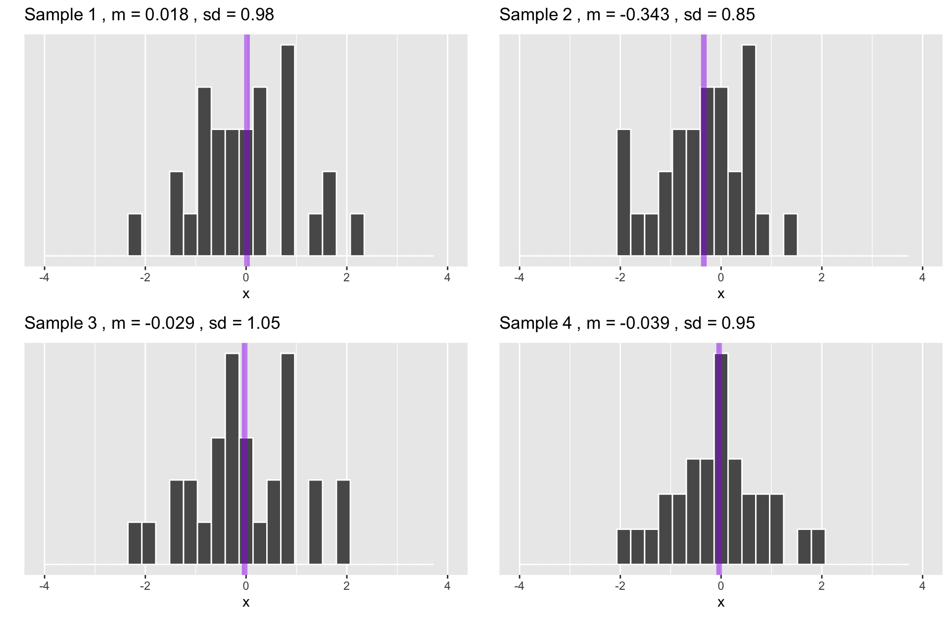
We use features of the sample (statistics) to inform us about features of the population (parameters). The quality of this information goes up as sample size goes up – the Law of Large Numbers. The quality of this information is easier to defend with random samples.
All sample statistics are wrong (they do not match the population parameters exactly) but they become more useful (better matches) as sample size increases.
An important practical question is “how big does the sample need to be?” Stated another way, “for a given sample size, how precise is a sample statistic as a representation of the population?”
The sampling distribution provides the answers.
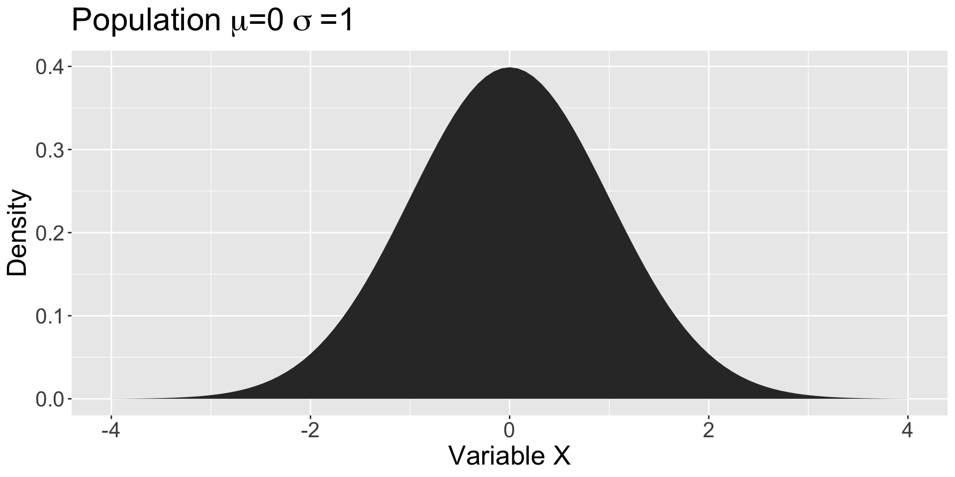
Population distribution
The parameters of this distribution are unknown. We use the sample to inform us about the likely characteristics of the population.
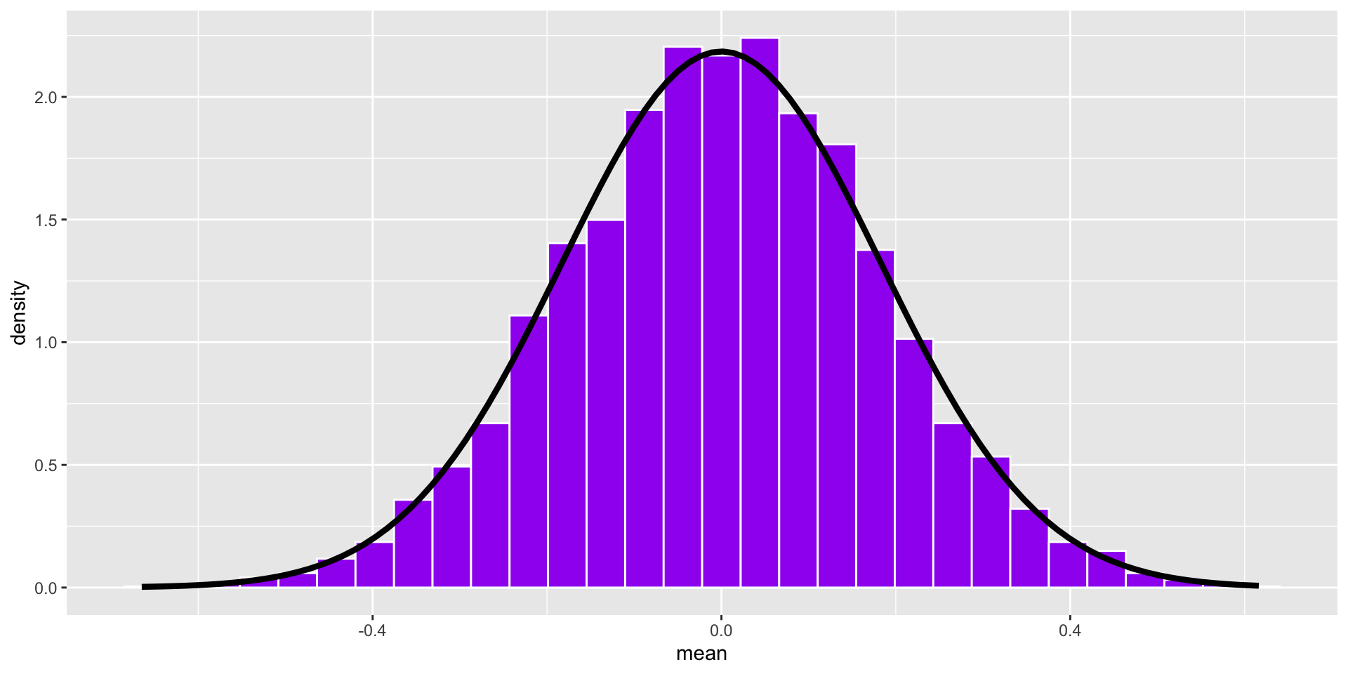
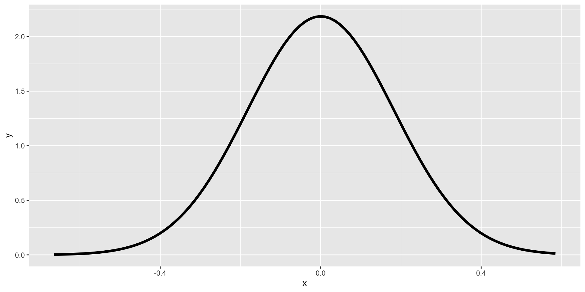
We don’t actually have to take a large number of random samples to construct the sampling distribution. It is a theoretical result of the Central Limit Theorem. We just need an estimate of the population parameter, \(s\), which we can get from the sample.
We don’t actually have to take a large number of random samples to construct the sampling distribution. It is a theoretical result of the Central Limit Theorem. We just need an estimate of the population parameter, \(s\), which we can get from the sample.
Code
ggplot(data.frame(x =seq(min(means), max(means), by = .05)), aes(x)) +stat_function(fun =function(x) dnorm(x, mean =0, sd = se), size =1.5)
The sampling distribution of means can be used to make probabilistic statements about means in the same way that the standard normal distribution is used to make probabilistic statements about scores.
For example, we can determine the range within which the population mean is likely to be with a particular level of confidence.
Or, we can propose different values for the population mean and ask how typical or rare the sample mean would be if that population value were true. We can then compare the plausibility of different such “models” of the population.
The key is that we have a sampling distribution of the mean with a standard deviation (the SEM) that is linked to the population:
\[SEM = \sigma_M = \frac{\sigma}{\sqrt{N}}\]
We do not know \(\sigma\) but we can estimate it based on the sample statistic:
\[\hat{\sigma} = s = \sqrt{\frac{1}{N-1}\sum_{i=1}^N(X-\bar{X})^2}\]
\[\hat{\sigma} = s = \sqrt{\frac{1}{N-1}\sum_{i=1}^N(X-\bar{X})^2}\]
This is the sample estimate of the population standard deviation. This is an unbiased estimate of \(\sigma\) and relies on the sample mean, which is an unbiased estimate of \(\mu\).
\[SEM = \sigma_M = \frac{\hat{\sigma}}{\sqrt{N}} = \frac{\text{Estimate of pop SD}}{\sqrt{N}}\] (Most methods of calculating standard deviation assume you’re estimating the population \(\sigma\) from a sample and correct for bias.)
The sampling distribution of the mean has variability, represented by the SEM, reflecting uncertainty in the sample mean as an estimate of the population mean.
The assumption of normality allows us to construct an interval within which we have good reason to believe a sample mean will fall if it comes from a particular population:
This is referred to as a 95% confidence interval (CI). Note the assumption of normality, which should hold by the Central Limit Theorem, if N is sufficiently large.
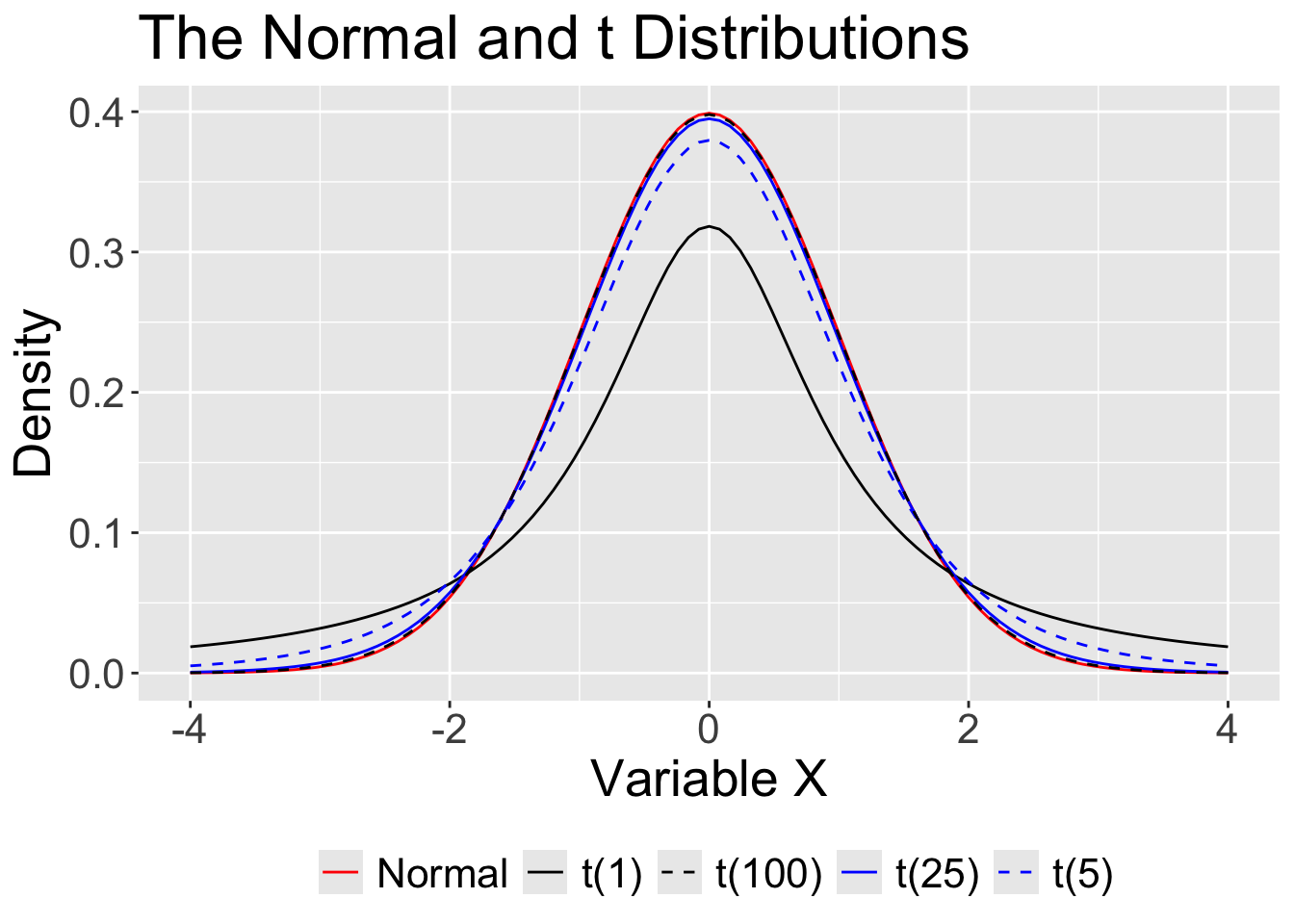
What if N is not “sufficiently large?” The normal distribution assumes we know the population mean and standard deviation. But we don’t. We only know the sample mean and standard deviation, and those have some uncertainty about them.
That uncertainty is reduced with large samples, so that the normal is “close enough.” In small samples, the t distribution provides a better approximation.
For small samples, we need to use the t distribution with its fatter tails. This produces wider confidence intervals—the penalty we have to pay for our ignorance about the population. The form of the confidence interval remains the same. We simply substitute a corresponding value from the t distribution (using df = \(N -1\)).
The meaning of the confidence interval can be a bit confusing and arises from the peculiar language forced on us by the frequentist viewpoint.
The CI DOES NOT mean “there is a 95% probability that the true mean lies inside the confidence interval.”
It means that if we carried out random sampling from the population a large number of times, and calculated the 95% confidence interval each time, then 95% of those intervals can be expected to contain the population mean. (Ugh, maybe those smug Bayesians are on to something.)
Maybe less tortured: We have good reason to believe the true mean lies in this interval because 95% of the time such intervals contain the true mean.
And even that interpretation is problematic, because it assumes our estimate of the standard deviation is error-free.
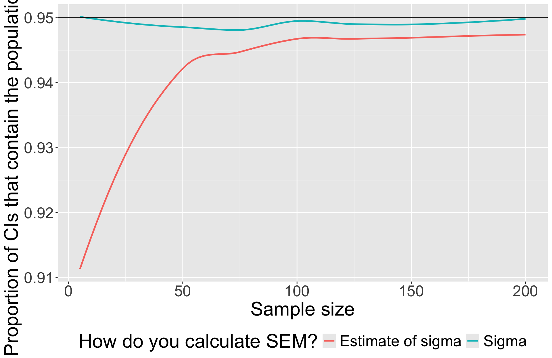
Simulation
At each sample size, draw 5000 samples from known population ( \(\mu = 0\) , \(\sigma = 1\) ). Calculate CI for each sample using \(s\) and record whether or not 0 was in that interval. Calculate CI using for each sample using \(\sigma\).
Code
reps =5000sizes =seq(5,200,5)prop =rep(0, length(sizes))prop_sig =rep(0, length(sizes))set.seed(101919)for(n in1:length(sizes)){ sample_size = sizes[n] correct =vector(length = reps) correct_sig =vector(length = reps)for(i in1:reps){ sample =rnorm(sample_size) m =mean(sample) s =sd(sample) sm = s/sqrt(sample_size) lb = m-(1.96*sm) ub = m+(1.96*sm) missed = lb >0| ub <0 correct[i] =!missed sigma =1 sm_sig = sigma/sqrt(sample_size) lb_sig = m-(1.96*sm_sig) ub_sig = m+(1.96*sm_sig) missed_sig = lb_sig >0| ub_sig <0 correct_sig[i] =!missed_sig } prop[n] =sum(correct)/reps prop_sig[n] =sum(correct_sig)/reps}data.frame(n = sizes, p = prop, ps = prop_sig) %>%gather("estimate", "value", -n) %>%mutate(estimate =ifelse(estimate =="p", "Estimate of sigma", "Sigma")) %>%ggplot(aes(x = n, y = value, color = estimate)) +geom_smooth( se = F) +geom_hline(aes(yintercept = .95), color ="black") +scale_color_discrete("How do you calculate SEM?") +labs(x ="Sample size", y ="Proportion of CIs that contain the population mean") +theme(text =element_text(size =25), legend.position ="bottom")
In the past, my classroom exams (aggregating over many classes) have a mean of 90 and a standard deviation of 8.
My next class will have 100 students. What range of exam means would be plausible if this class is similar to past classes (comes from the same population)?
M =90SD =8N =100sem = SD/sqrt(N)ci_lb_z = M - sem *qnorm(p = .975)ci_ub_z = M + sem *qnorm(p = .975)print(c(ci_lb_z, ci_ub_z))
[1] 88.43203 91.56797
ci_lb_z = M - sem *qt(p = .975, df = N-1)ci_ub_z = M + sem *qt(p = .975, df = N-1)print(c(ci_lb_z, ci_ub_z))
[1] 88.41263 91.58737
I give a classroom exam that produces a mean of 83.4 and a standard deviation of 10.6. A total of 26 students took the exam.
What is the 95% confidence interval around the mean?
What kinds of population inferences can I draw?
M =83.4SD =10.6N =26sem = SD/sqrt(N)ci_lb_z = M - sem *qnorm(p = .975)ci_ub_z = M + sem *qnorm(p = .975)print(c(ci_lb_z, ci_ub_z))
[1] 79.32557 87.47443
ci_lb_z = M - sem *qt(p = .975, df = N-1)ci_ub_z = M + sem *qt(p = .975, df = N-1)print(c(ci_lb_z, ci_ub_z))