More NHST
We collect a sample and compare this to a null hypothesis: \(H_0: \mu_0 = 100\). Holding our sample mean \((\bar{X} = 105)\) constant, how does our \(p\)-value change as our sample size gets larger?
Code
x_vals = seq(85, 115, by = .05)

data.frame(
  m = 100,
  s = 15,
  n = seq(5, 150, 5)) %>%
  mutate(
    X = map(n, ~x_vals),
    density = map(n, ~dnorm(x = x_vals, m = 100, s = 15/sqrt(.x))),
    pvalue = map(n, ~pnorm(5/(15/sqrt(.x)), lower.tail = F)*2),
    pvalue = map_chr(pvalue, papaja::printp)) %>%
  unnest(cols = c(X, density)) %>%
ggplot(aes(x=X, y=density, frame=n)) +
  geom_line() +
  geom_vline(aes(xintercept = 105), color = "purple") +
  geom_label(aes(x = 107, y = .2, label = paste("p:", pvalue)), hjust = 0) +
  labs(x = "X",
       y = "density",
       title = "N = {closest_state}") +
  transition_states(n,
                    transition_length = 10,
                    state_length = 2) +
  theme_pubr()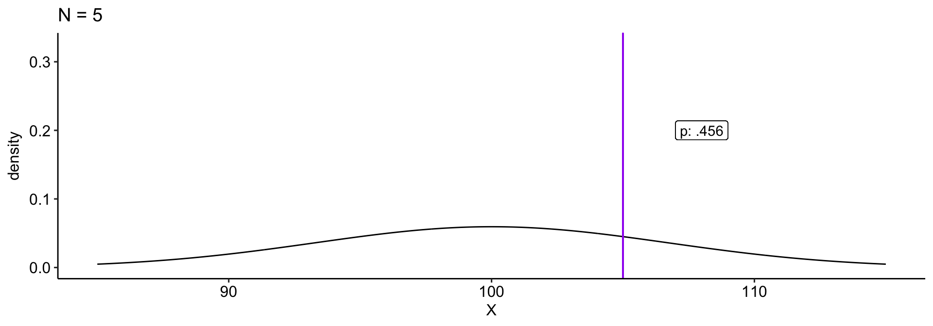
We begin by defining the location in the null hypothesis distribution beyond which empirical results would be considered sufficiently unusual to lead us to reject the null hypothesis. We control these mistakes (Type I errors) at the chosen level of significance ( \(\alpha = .05\) ).
Code
mu = 100
xbar = 110
s = 20
n = 25
sem = s/sqrt(n)
cv = qnorm(mean = mu, sd = sem, p = .025, lower.tail = F)
cv2 = qnorm(mean = mu, sd = sem, p = .025, lower.tail = T)

ggplot(data.frame(x = seq(70, 130)), aes(x)) +
  stat_function(fun = function(x) dnorm(x, m = mu, sd = sem)) +
  stat_function(fun = function(x) dnorm(x, m = mu, sd = sem),
                geom = "area", xlim = c(cv, 130), fill = "red") +
  geom_vline(aes(xintercept = cv), color = "red")+
  stat_function(fun = function(x) dnorm(x, m = mu, sd = sem),
                geom = "area", xlim = c(cv2, 70), fill = "red") +
  geom_vline(aes(xintercept = mu))+
  geom_hline(aes(yintercept = 0))+
  scale_x_continuous("Means", breaks = seq(70,130,10)) +
  scale_y_continuous(NULL, breaks = NULL)+
  theme_pubr() +
  theme(text = element_text(size = 20))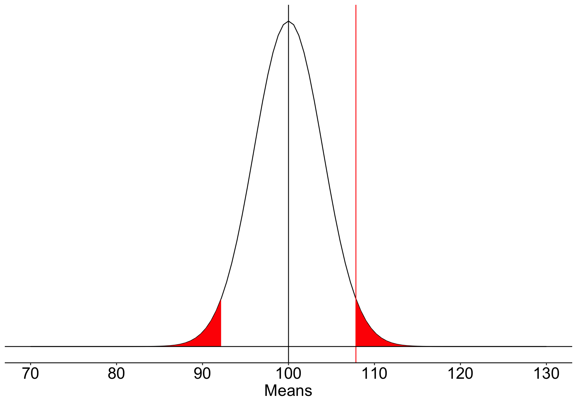
\[\small \text{Critical Value} \\= \mu_0 + Z_{.975}\frac{\sigma}{\sqrt{N}}\\= 100 + 1.96\frac{20}{\sqrt{25}} \\= 107.84\]
What if the null hypothesis is false? How likely are we to correctly reject the null hypothesis in the long run?
Code
mu = 100
xbar = 110
s = 20
n = 25
sem = s/sqrt(n)
cv = qnorm(mean = mu, sd = sem, p = .025, lower.tail = F)
cv2 = qnorm(mean = mu, sd = sem, p = .025, lower.tail = T)

ggplot(data.frame(x = seq(70, 130)), aes(x)) +
  stat_function(fun = function(x) dnorm(x, m = mu, sd = sem)) +
  stat_function(fun = function(x) dnorm(x, m = mu, sd = sem),
                geom = "area", xlim = c(cv, 130), fill = "red") +
  geom_vline(aes(xintercept = cv), color = "red")+
  stat_function(fun = function(x) dnorm(x, m = mu, sd = sem),
                geom = "area", xlim = c(cv2, 70), fill = "red") +
  geom_vline(aes(xintercept = mu))+
  geom_hline(aes(yintercept = 0))+
  scale_x_continuous("Means", breaks = seq(70,130,10)) +
  scale_y_continuous(NULL, breaks = NULL)+
  theme_pubr() +
  theme(text = element_text(size = 20))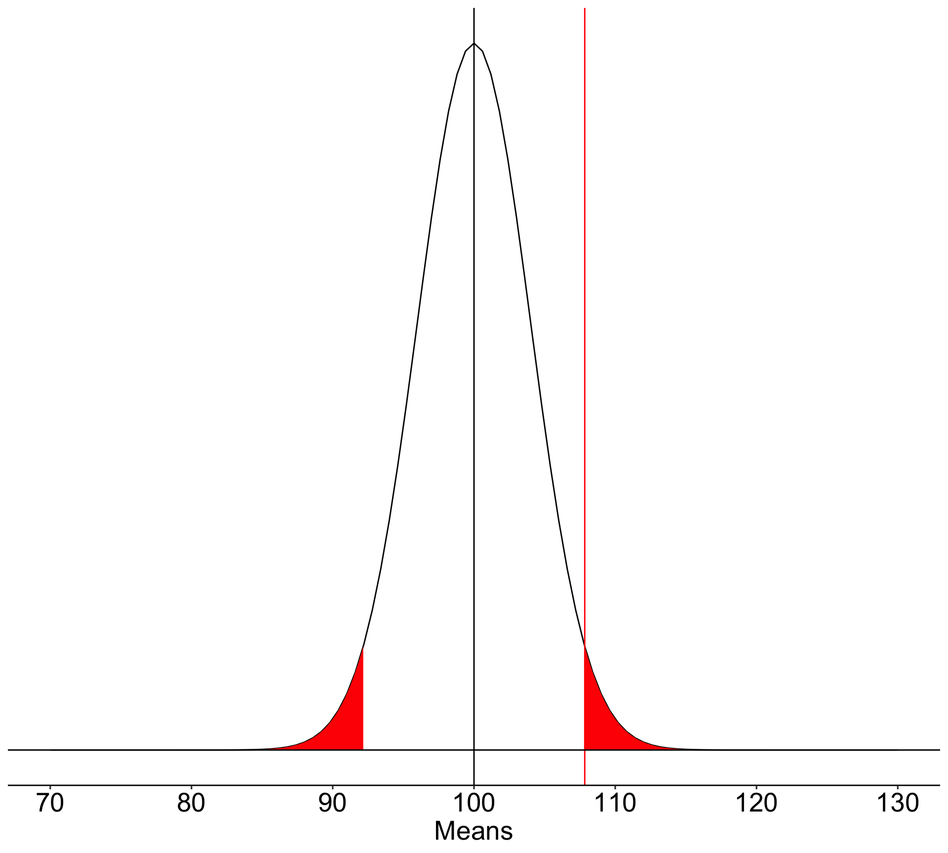
Code
data.frame(x = seq(70, 140)) %>%
  ggplot(aes(x = x)) +
  stat_function(fun = function(x) dnorm(x, mean = mu, sd = sem),
                 geom = "line") +
  stat_function(aes(fill = "Type I error"), fun = function(x) dnorm(x, mean = mu, sd = sem),
                 geom = "area", xlim = c(cv, 140),
                alpha = .5) +
  stat_function(aes(fill = "Type I error"), fun = function(x) dnorm(x, mean = mu, sd = sem),
                 geom = "area", xlim = c(70, cv2),
                alpha = .5) +
  geom_vline(aes(xintercept = cv, color = "Critical Value")) +
  guides(color = "none") +
  scale_x_continuous(limits = c(70,140), breaks = seq(70, 140, 10)) +
  scale_y_continuous(breaks = NULL) +
  labs(x = "Mean", y = "density", fill = NULL)+
  theme_pubr()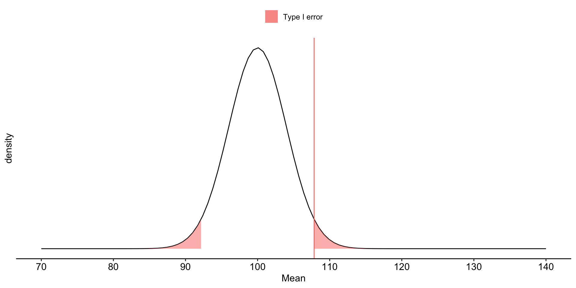
Code
data.frame(x = seq(70, 140)) %>%
  ggplot(aes(x = x)) +
  stat_function(fun = function(x) dnorm(x, mean = mu, sd = sem),
                 geom = "line", alpha = .2) +
  geom_vline(aes(xintercept = cv, color = "Critical Value")) +
  guides(color = "none") +
  scale_x_continuous(limits = c(70,140), breaks = seq(70, 140, 10)) +
  scale_y_continuous(breaks = NULL) +
  labs(x = "Mean", y = "density", fill = NULL)+
  theme_pubr()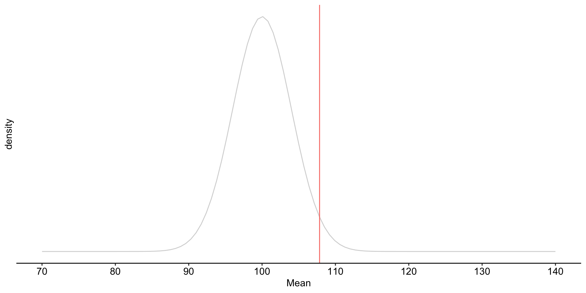
Code
data.frame(x = seq(70, 140)) %>%
  ggplot(aes(x = x)) +
  stat_function(fun = function(x) dnorm(x, mean = mu, sd = sem),
                 geom = "line", alpha = .2) +
  stat_function(fun = function(x) dnorm(x, mean = xbar, sd = sem),
                 geom = "line") +
  geom_vline(aes(xintercept = cv, color = "Critical Value")) +
  guides(color = "none") +
  scale_x_continuous(limits = c(70,140), breaks = seq(70, 140, 10)) +
  scale_y_continuous(breaks = NULL) +
  labs(x = "Mean", y = "density", fill = NULL)+
  theme_pubr()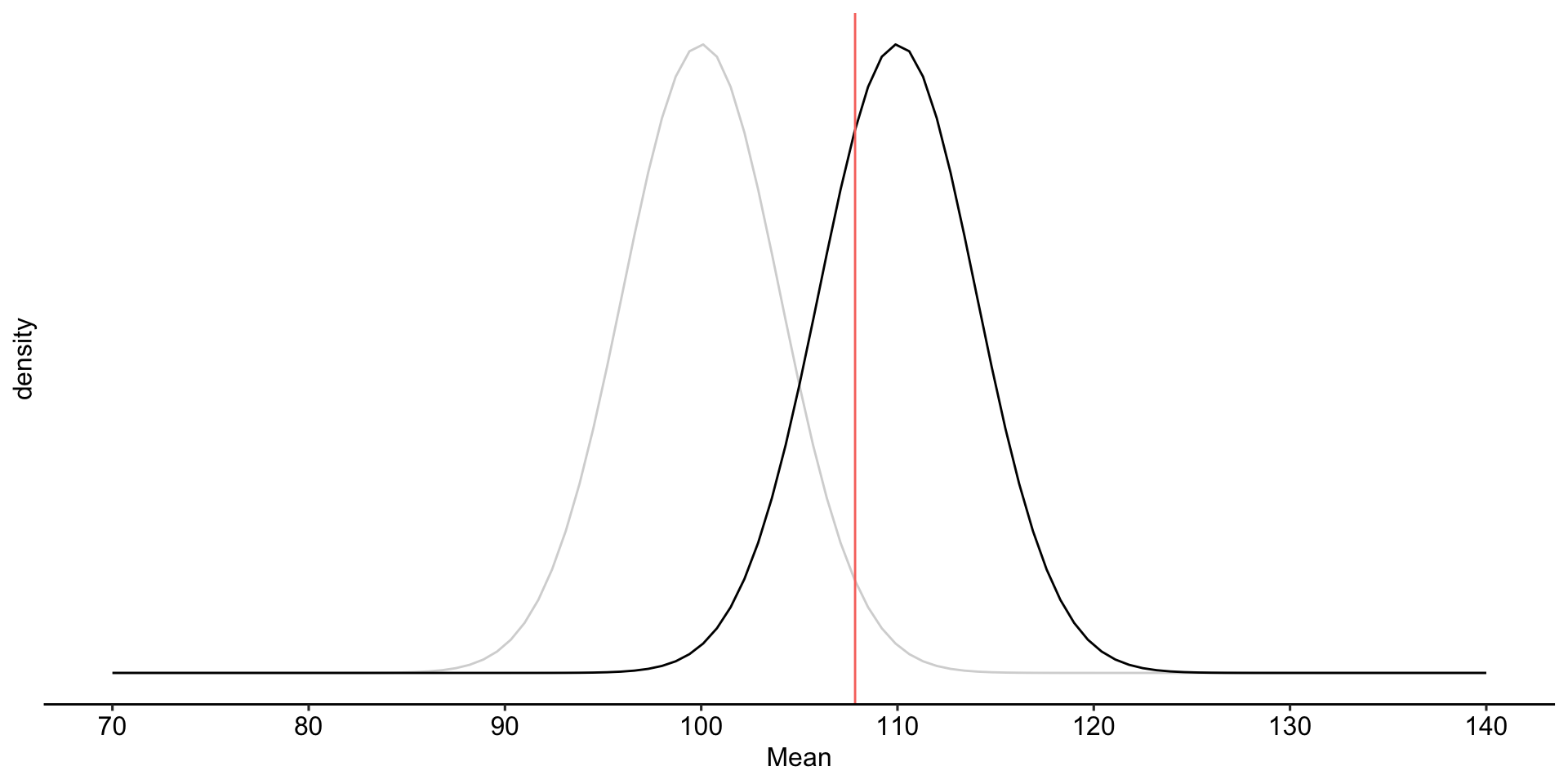
Code
data.frame(x = seq(70, 140)) %>%
  ggplot(aes(x = x)) +
  stat_function(fun = function(x) dnorm(x, mean = mu, sd = sem),
                 geom = "line", alpha = .2) +
  stat_function(fun = function(x) dnorm(x, mean = xbar, sd = sem),
                 geom = "line") +
  stat_function(aes(fill = "Power"), fun = function(x) dnorm(x, mean = xbar, sd = sem),
                 geom = "area", xlim = c(cv, 140),
                alpha = .5) +
  stat_function(aes(fill = "Type II error"), fun = function(x) dnorm(x, mean = xbar, sd = sem),
                 geom = "area", xlim = c(70, cv),
                alpha = .5) +
  geom_vline(aes(xintercept = cv, color = "Critical Value")) +
  guides(color = "none") +
  scale_x_continuous(limits = c(70,140), breaks = seq(70, 140, 10)) +
  scale_y_continuous(breaks = NULL) +
  labs(x = "Mean", y = "density", fill = NULL)+
  theme_pubr()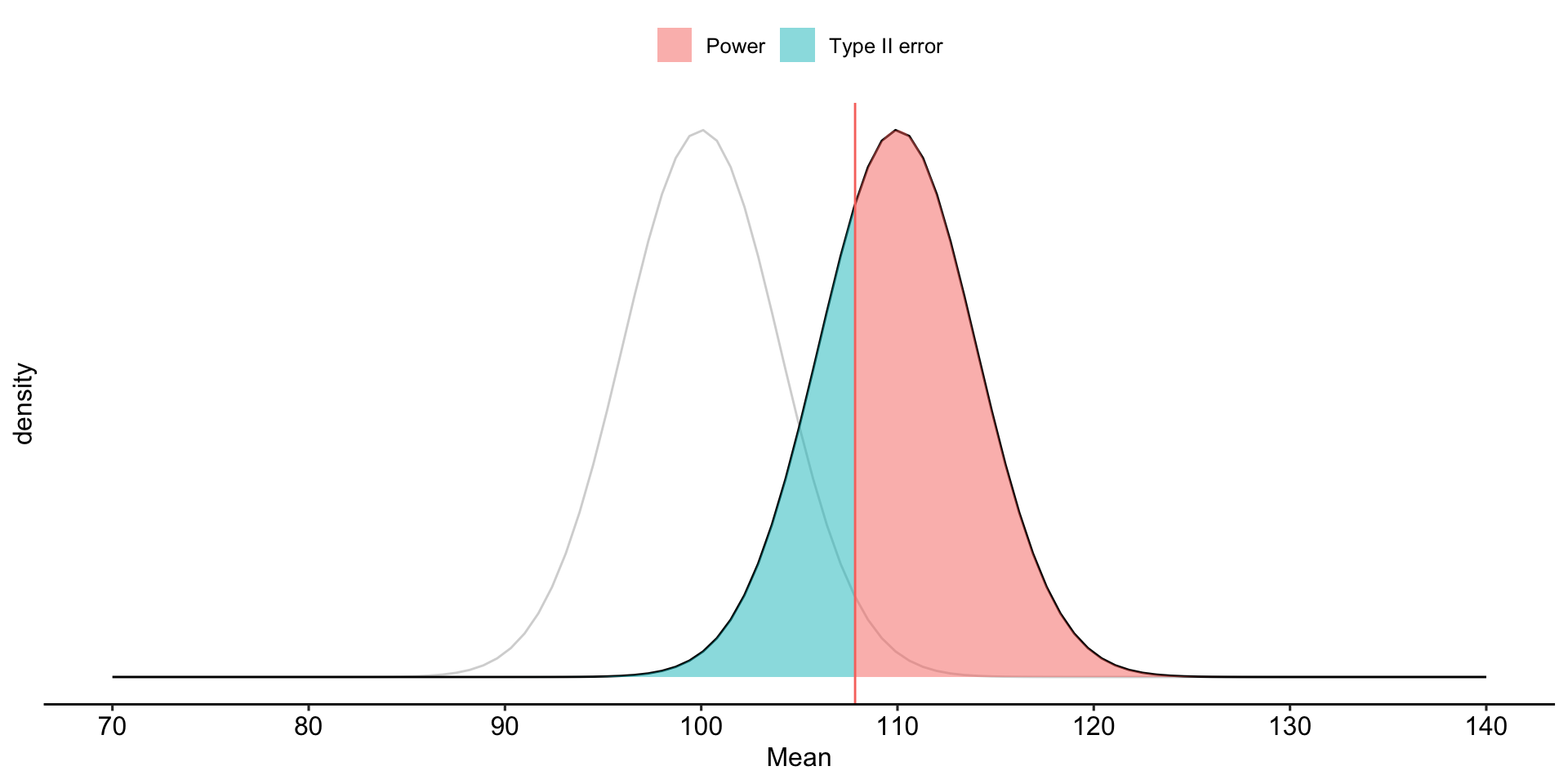
To determine the probability of a Type II error, we must specify a value for the alternative hypothesis. We will use the sample mean of 110.
In the long run, if psychology samples have a mean of 110 ( \(\sigma = 20\), \(N = 25\) ), we will correctly reject the null with probability of 0.71 (power). We will incorrectly fail to reject the null with probability of 0.29 ( \(\beta\) ).
Once the critical value and alternative value is established, we can determine the location of the critical value in the alternative distribution.
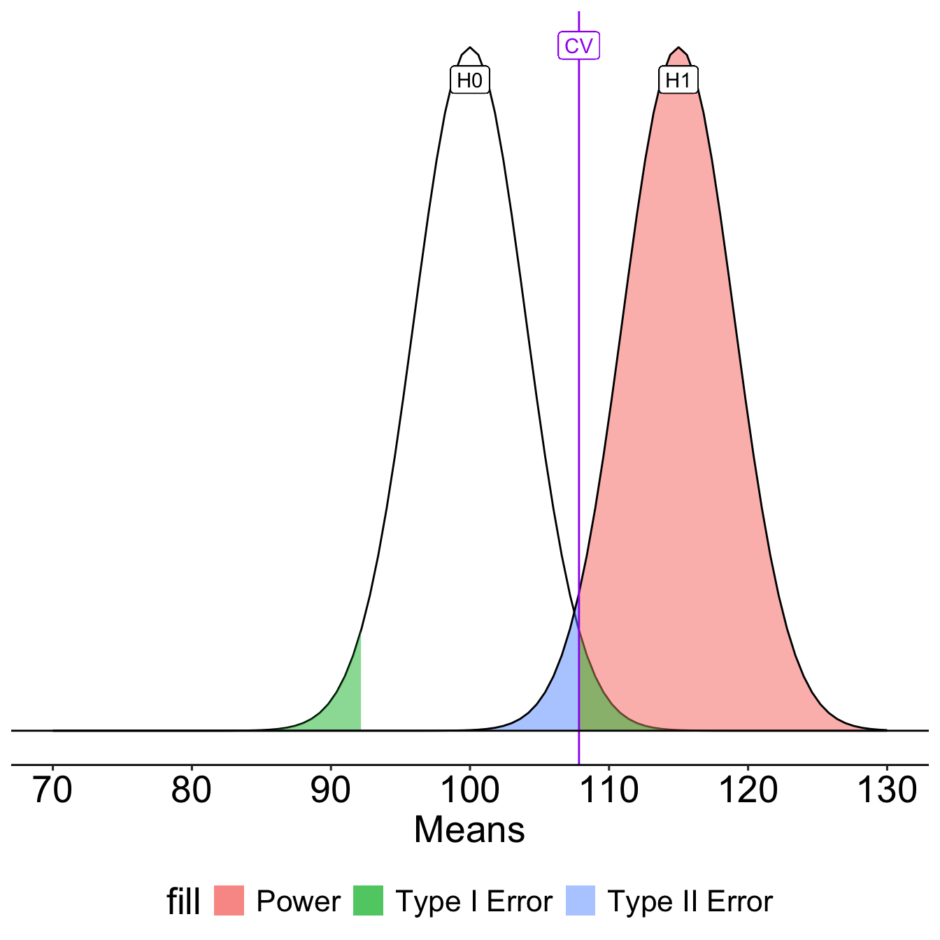
[1] -0.540036The choice of 110 as the mean of \(H_1\) is completely arbitrary. What if we believe that the alternative mean is 115? This larger signal should be easier to detect.
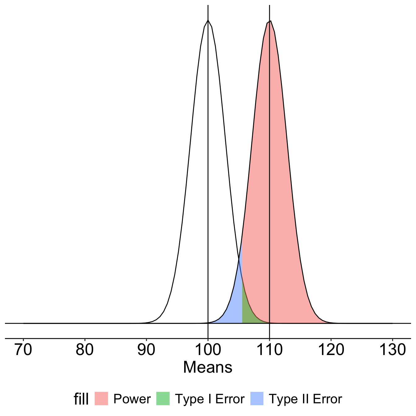
What if instead we increase the sample size? This will reduce variability in the sampling distribution, making the difference between the null and alternative distributions easier to see. (New \(N\) is 50.)
What if we decrease the significance level to .01?
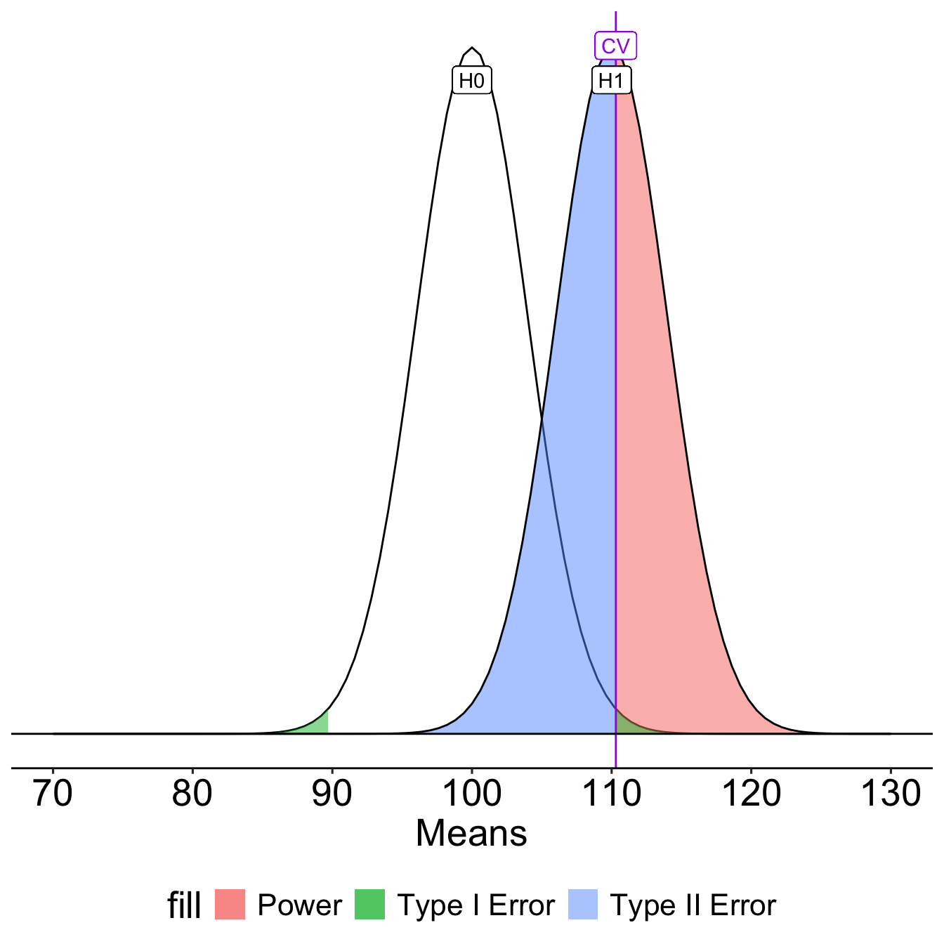
Oops, we’ve been ignoring the other tail. So far it hasn’t mattered (the area has been so small) but it makes a difference when \(H_0\) and \(H_1\) overlap significantly.
More generally we can determine the relationship between effect size and power for a constant \(\alpha\) (.05) and sample size ( \(N = 20\) ).
Code
pwr_fun = function(m1, m2, alpha, n, sd){
  sem = sd/sqrt(n)
  cv = qnorm(p = 1-(alpha/2), mean = m1, sd = sem)
  z_1 = (cv-m2)/sem
  power = pnorm(q = z_1, lower.tail = F)
  return(power)
}

size = seq(100, 120, 1)

data.frame(effect = size, power = sapply(size, function(x) pwr_fun(m1 = 100, m2 = x, alpha = .05, n = 20, sd = 20))) %>%
  ggplot(aes(x = effect, y = power)) +
  geom_line(size = 1.5) +
  scale_x_continuous(expression(H[1]~Mean)) +
  ggtitle("Power to detect significant effect by mean") +
  theme_pubr() +
  theme(text = element_text(size = 20))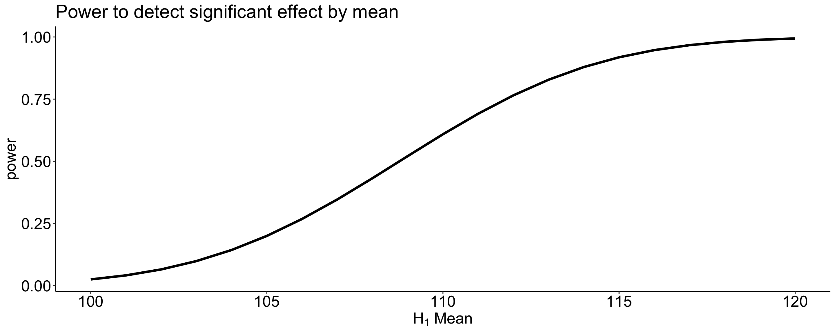
Likewise, we can display the relationship between sample size and power for a constant \(\alpha\) and effect size.
Code
size = seq(5,200,5)

data.frame(size = size, power = sapply(size, function(x) pwr_fun(m1 = 100, m2 = 110, alpha = .05, n = x, sd = 20))) %>%
  ggplot(aes(x = size, y = power)) +
  geom_line(size = 1.5) +
  scale_x_continuous("Sample Size") +
  ggtitle("Power to detect significant effect by sample size") +
  theme_pubr() +
  theme(text = element_text(size = 20))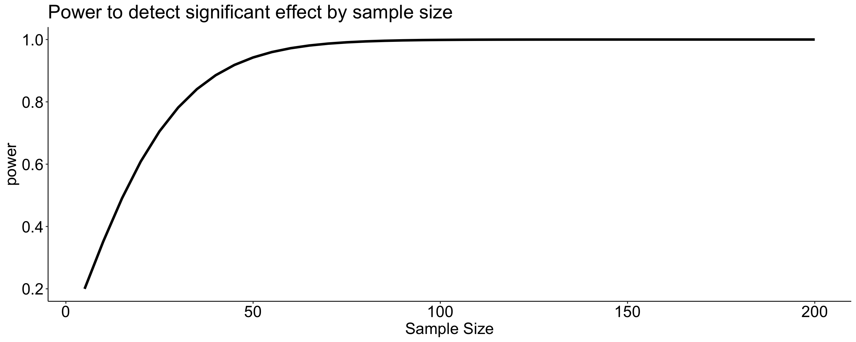
Power changes as a function of significance level for a constant effect size and sample size.
Code
size = seq(.01,.20,.01)

data.frame(alpha = size,
           power = sapply(size, function(x) pwr_fun(m1 = 100,
                                                    m2 = 110,
                                                    alpha = x,
                                                    n = 20,
                                                    sd = 20))) %>%
  ggplot(aes(x = alpha, y = power)) +
  geom_line(size = 1.5) +
  scale_x_continuous(expression(alpha)) +
  ggtitle("Power to detect significant effect by alpha") +
  theme_pubr() +
  theme(text = element_text(size = 20))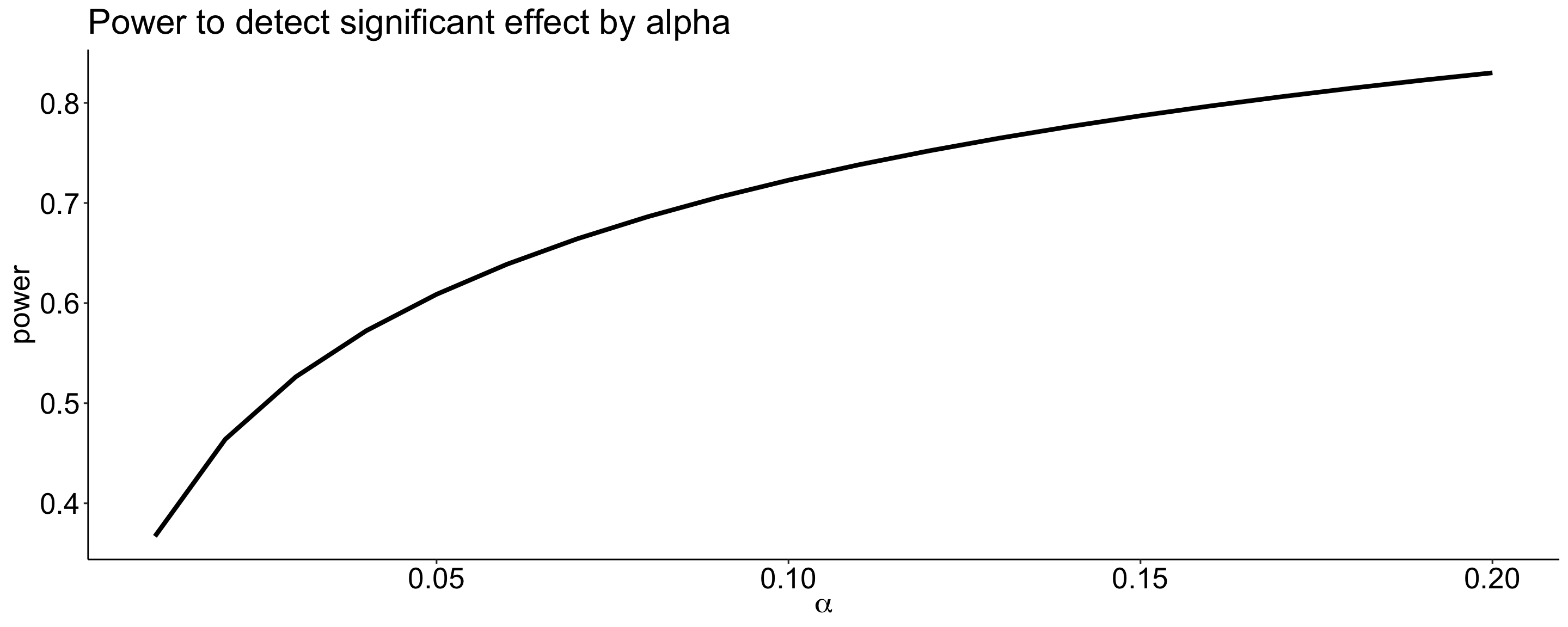
For a one-tailed test, we put the entire rejection area into a single tail. If \(\alpha = .05\), then one tail contains .05 and critical values will be either 1.64 or -1.64 standard errors away from the null mean.
Code
mu = 100
x = 110
s = 20
n = 25
sem = s/sqrt(n)
cv_sngle = qnorm(mean = mu, sd = sem, p = .05, lower.tail = F)

ggplot(data.frame(x = seq(70, 130)), aes(x)) +
  stat_function(fun = function(x) dnorm(x, m = mu, sd = sem)) +
  stat_function(fun = function(x) dnorm(x, m = mu, sd = sem),
                geom = "area", xlim = c(cv_sngle, 130), fill = "red") +
  geom_vline(aes(xintercept = cv_sngle), color = "red")+
  geom_vline(aes(xintercept = mu))+
  geom_hline(aes(yintercept = 0))+
  scale_x_continuous("Means", breaks = seq(70,130,10)) +
  scale_y_continuous(NULL, breaks = NULL) +
  theme_pubr() +
  theme(text = element_text(size = 20))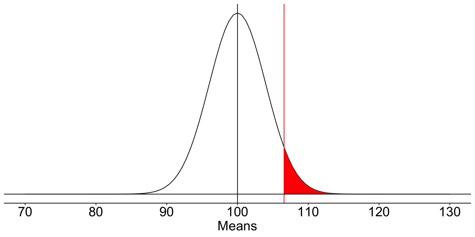
A two-tailed test is less powerful (more conservative) than a one-tailed test for the same sample size.
Code
pwr1_fun = function(m1, m2, alpha, n, sd){
  sem = sd/sqrt(n)
  cv = qnorm(p = 1-(alpha), mean = m1, sd = sem)
  z_1 = (cv-m2)/sem
  power = pnorm(q = z_1, lower.tail = F)
  return(power)
}
pwr2_fun = function(m1, m2, alpha, n, sd){
  sem = sd/sqrt(n)
  cv_1 = qnorm(p = 1-(alpha/2), mean = m1, sd = sem)
  cv_2 = qnorm(p = (alpha/2), mean = m1, sd = sem)
  z_1 = (cv_1-m2)/sem
  z_2 = (cv_2-m2)/sem
  power = pnorm(q = z_1, lower.tail = F) + pnorm(q = z_2, lower.tail = T)
  return(power)
}

size = seq(5,100,5)

data.frame(effect = size,
           power_1 = sapply(size, function(x) pwr1_fun(m1 = 100, m2 = 110, alpha = .05, n = x, sd = 20)),
           power_2 = sapply(size, function(x) pwr2_fun(m1 = 100, m2 = 110, alpha = .05, n = x, sd = 20))) %>%
  ggplot(aes(x = effect)) +
  geom_line(aes(y = power_1, color = "one-tail"), size = 1.5) +
  geom_line(aes(y = power_2, color = "two-tail"), size = 1.5) +
  scale_x_continuous("Sample Size") +
  scale_y_continuous("power")+
  ggtitle("Power to detect significant effect by mean") +
  theme_pubr() +
  theme(text = element_text(size = 20))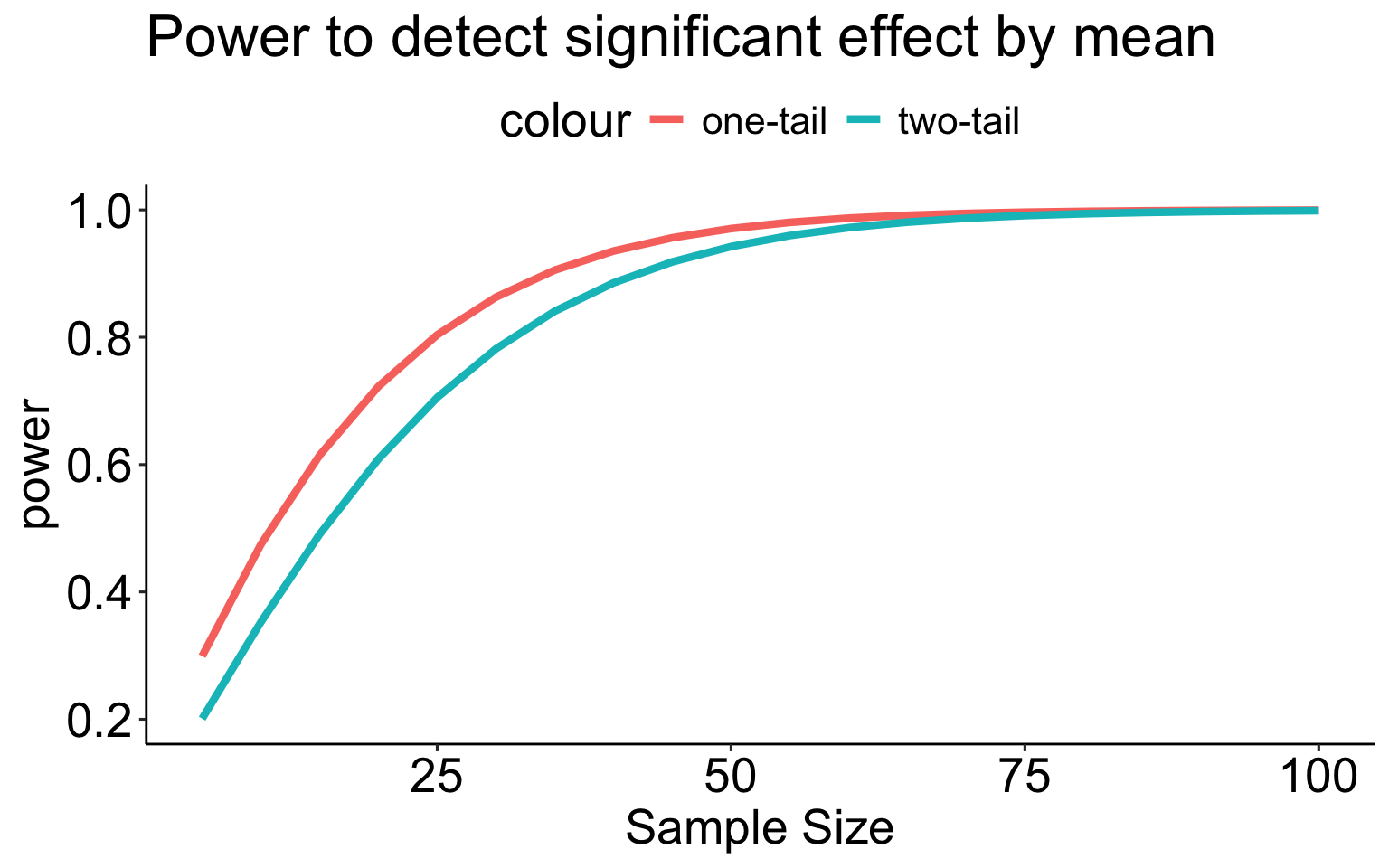
Code
means = data.frame(means = seq(101, 115, .2)) %>%
  mutate(d = abs(means-100)/20)
means$power_1 = sapply(means$d, function(x) pwr.norm.test(d = x, sig.level = .05, power = .80, alternative = "greater")$n)
means$power_2 = sapply(means$d, function(x) pwr.norm.test(d = x, sig.level = .05, power = .80, alternative = "two.sided")$n)

means %>%
  ggplot(aes(x = means)) +
  geom_line(aes(y=power_1, color = "one-tailed"), size = 1.5) +
  geom_line(aes(y=power_2, color = "two-tailed"), size = 1.5) +
  scale_x_continuous(expression(H[1]~Mean))+
  scale_y_continuous("Sample size needed") +
  theme_pubr() +
  theme(text = element_text(size = 20))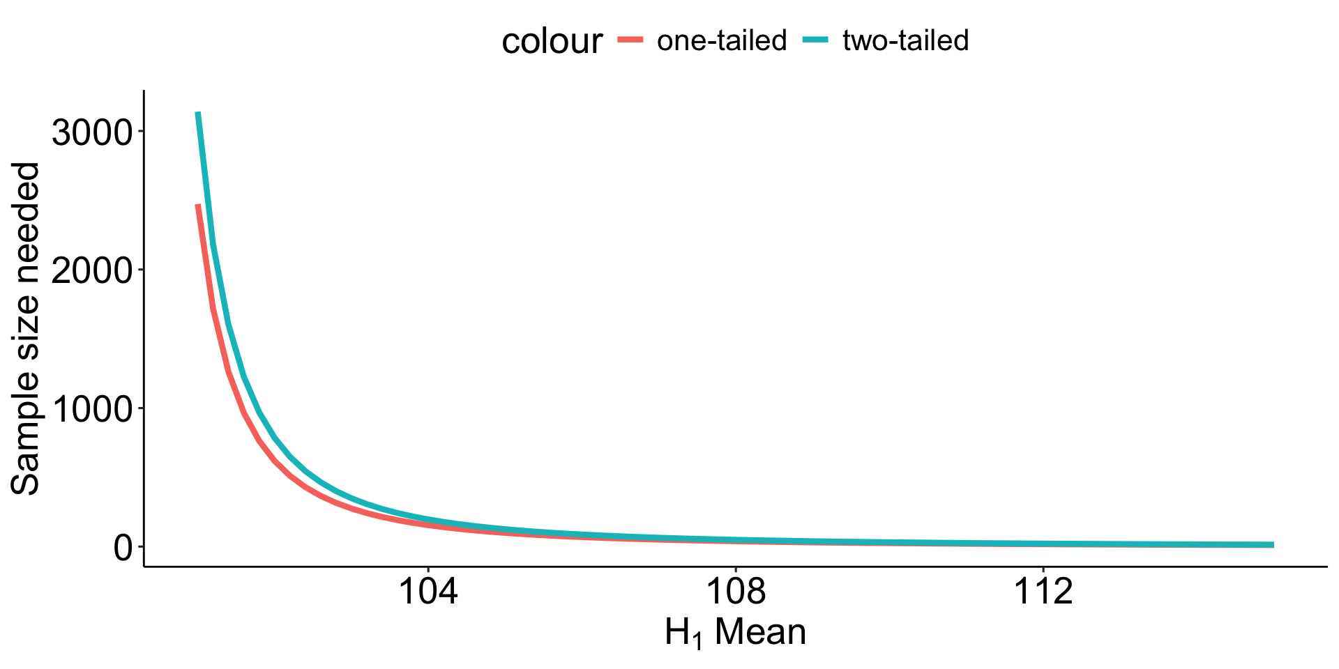
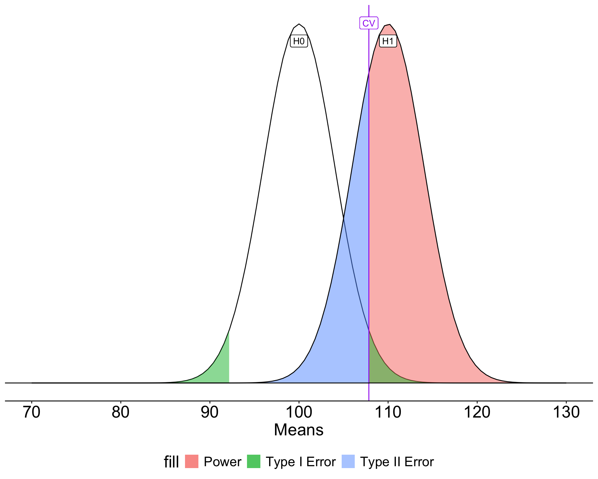
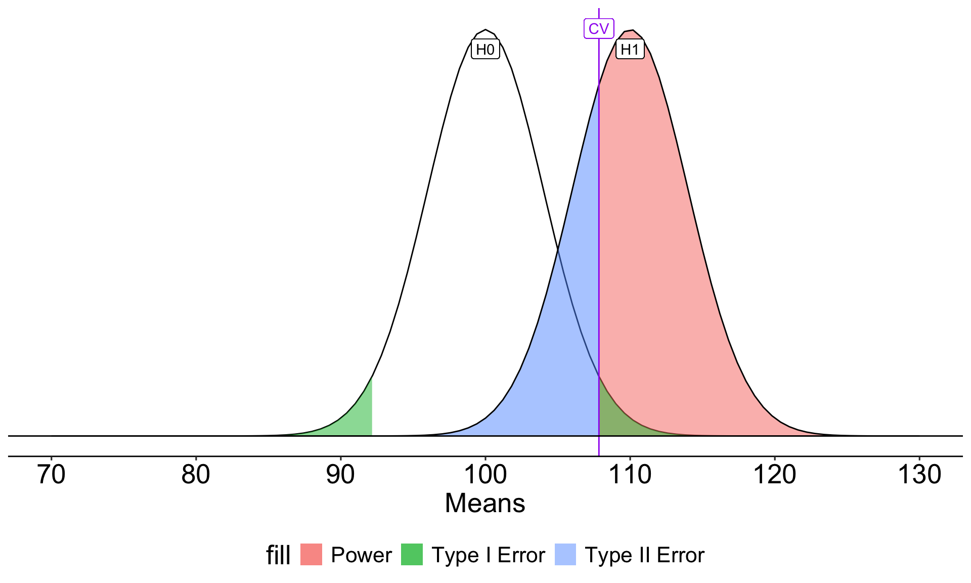
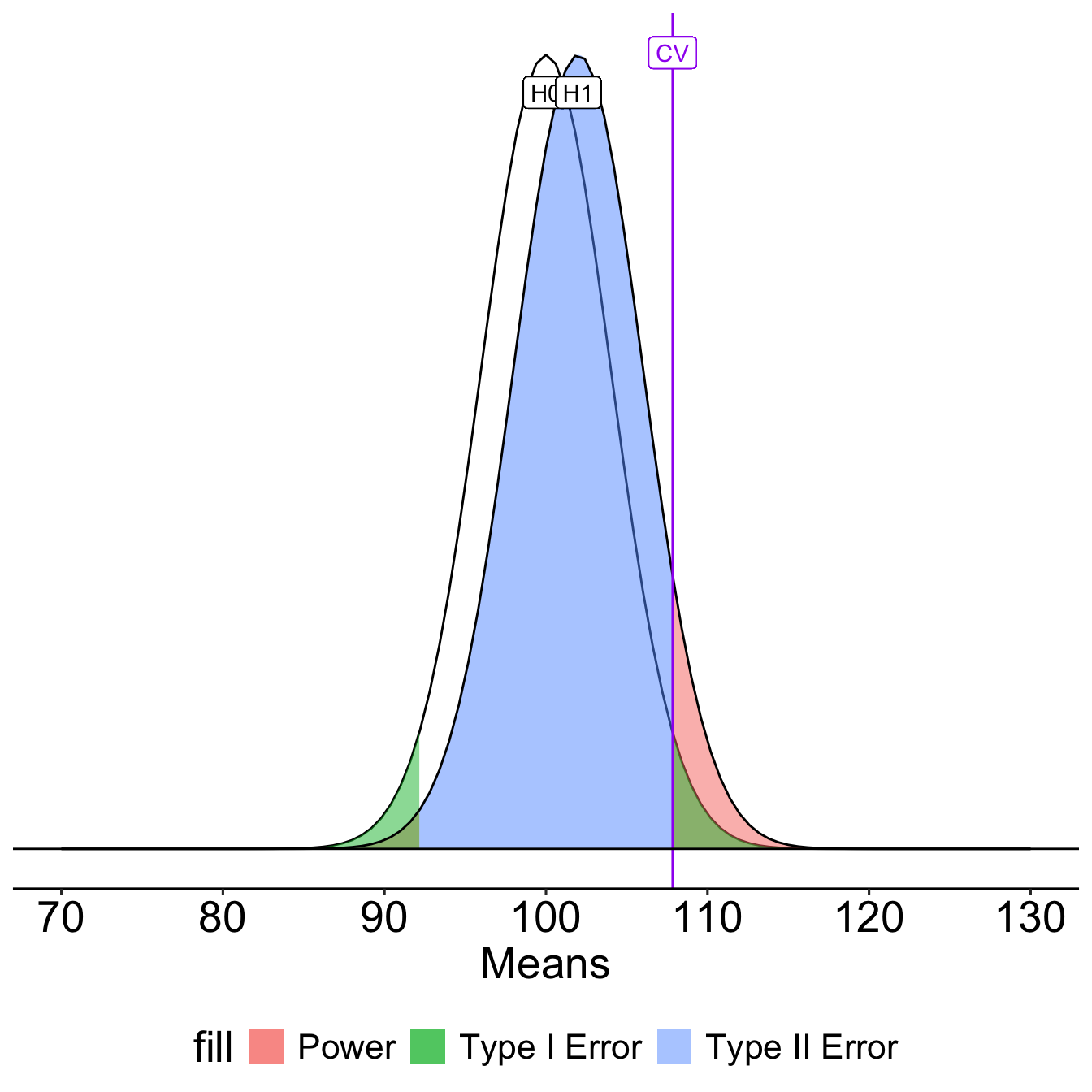
How can power be increased?
Code
#|
ggplot(data.frame(x = seq(70, 130)), aes(x)) +
  stat_function(fun = function(x) dnorm(x, m = mu, sd = sem)) +

  stat_function(fun = function(x) dnorm(x, m = mean, sd = sem),
                geom = "area", xlim = c(cv, 130),
                aes(fill = "Power"), alpha = .5) +
  stat_function(fun = function(x) dnorm(x, m = mean, sd = sem),
                geom = "area", xlim = c(70, cv2),
                aes(fill = "Power"), alpha = .5) +
  stat_function(fun = function(x) dnorm(x, m = mean, sd = sem),
                geom = "area", xlim = c(cv2, cv),
                aes(fill = "Type II Error"), alpha = .5) +
  stat_function(fun = function(x) dnorm(x, m = mu, sd = sem),
                geom = "area", xlim = c(cv, 130),
                aes(fill = "Type I Error"), alpha = .5) +
  stat_function(fun = function(x) dnorm(x, m = mu, sd = sem),
                geom = "area", xlim = c(cv2, 70),
                aes(fill = "Type I Error"), alpha = .5) +
  stat_function(fun = function(x) dnorm(x, m = mean, sd = sem)) +
  geom_vline(aes(xintercept = cv), color = "purple")+
  geom_label(aes(x = mu, y = .095, label = "H0")) +
  geom_label(aes(x = mean, y = .095, label = "H1")) +
  geom_label(aes(x = cv, y = .1, label = "CV"), color = "purple") +
  geom_hline(aes(yintercept = 0))+
  scale_x_continuous("Means", breaks = seq(70,130,10)) +
  scale_y_continuous(NULL, breaks = NULL) +
  theme_pubr() +
  theme( text = element_text(size = 20),
    legend.position = "bottom")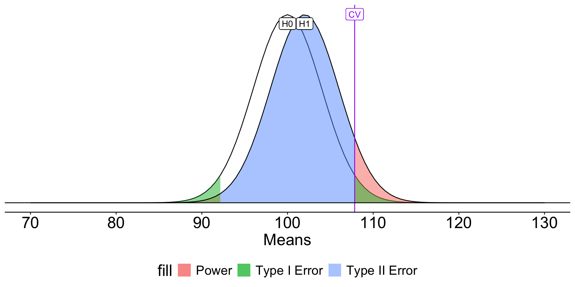
\[Z_1 = \frac{CV_0 - \mu_1}{\frac{\sigma}{\sqrt{N}}}\]
- increase \(\mu_1\)
- decrease \(CV_0\)
- increase \(N\)
- reduce \(\sigma\)
I strongly recommend playing around with different configurations of \(N\), \(\alpha\) and the difference in means ( \(d\) ) in this online demo.