Paired-sample tests

Announcements

• Oral Exam questions posted next week
• Oral exam time slots open next week – please sign up before Monday Dec 2!
• Send requests for Tuesday’s lecture.

Previously…

• chi-square \((\chi^2) tests\)
• One-sample t-tests

Today

• Paired-samples t-tests

library(here)
library(tidyverse)
library(ggpubr)
library(knitr)
library(kableExtra)

In longitudinal research, the same people provide responses to the same measure on two occasions (the individuals in the two groups are the same).

In paired-sample research, the individuals in the two groups are different, but they are related and their responses are assumed to be correlated. Examples would be responses by children and their parents, members of couples, twins, etc.

In paired-measures research, the same people provide responses to two different measures that assess closely related constructs. This resembles longitudinal research, but data collection occurs at one time.

All of these are instances of repeated measures designs.

The advantage of repeated measures designs is that, compared to an independent groups design of the same size, the repeated measures design is more powerful.

• Two groups are more alike than in simple randomization

• The correlated sampling units will have less variability on “nuisance variables” because those are either the same over time (longitudinal) or over measures (paired measures), or very similar over people (paired samples).

• Nuisance variables – anything that isn’t relevant to the study.

Each of these repeated measures problems can be viewed as a transformation of the original two measures into a single measure: a difference score. This reduces the analysis to a one-sample t-test on the difference score, with null mean = 0.

If the repeated measures are \(X_1\) and \(X_2\), then their difference is \(D = X_1 – X_2\). This new measure has a mean and standard deviation, like any other single measure, making it appropriate for a one-sample t-test.

\[t_{df = N-1} = \frac{\bar{\Delta}-\mu}{\frac{\hat{\sigma}_\Delta}{\sqrt{N}}}\]

\[H_0: \bar{\Delta} = \mu\] \[H_1: \bar{\Delta} \neq \mu\]

\[H_0: \bar{\Delta} = 0\] \[H_1: \bar{\Delta} \neq 0\]

Note here the signal to noise ratios

Example 1: Gulls

Human-wildlife conflict in urban areas endangers wildlife species. One species under threat is the Larus argentatus or herring gull, which is considered a nuisance owing to food-snatching and other behaviors. A recent study examined whether herring gull behavior is influenced by human behavior cues and whether this could be used to reduce human-gull conflict.

Example 1: Gulls

In this study, experimenters visited coastal towns in the UK and found locations with multiple gulls. They placed a bag of potato chips (250 g) in front of them and measured how long it took gulls to peck at the food.

“We adopted a repeated measures design… We randomly assigned individuals to receive Looking At or Looking Away first, and trial order was counterbalanced across individuals. Second trials commenced 180 s after the completion of the first trial to allow normal behaviour to resume.”

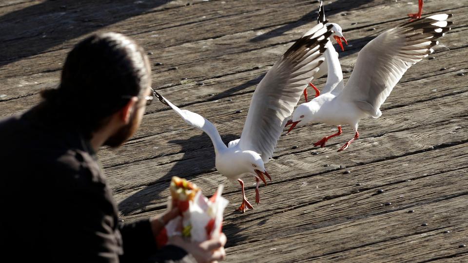
In the Looking At treatment, the experimenter directed her gaze towards the eye(s) of the gull and turned her head, if necessary, to follow its approach path until the gull completed the trial by pecking at the food bag.

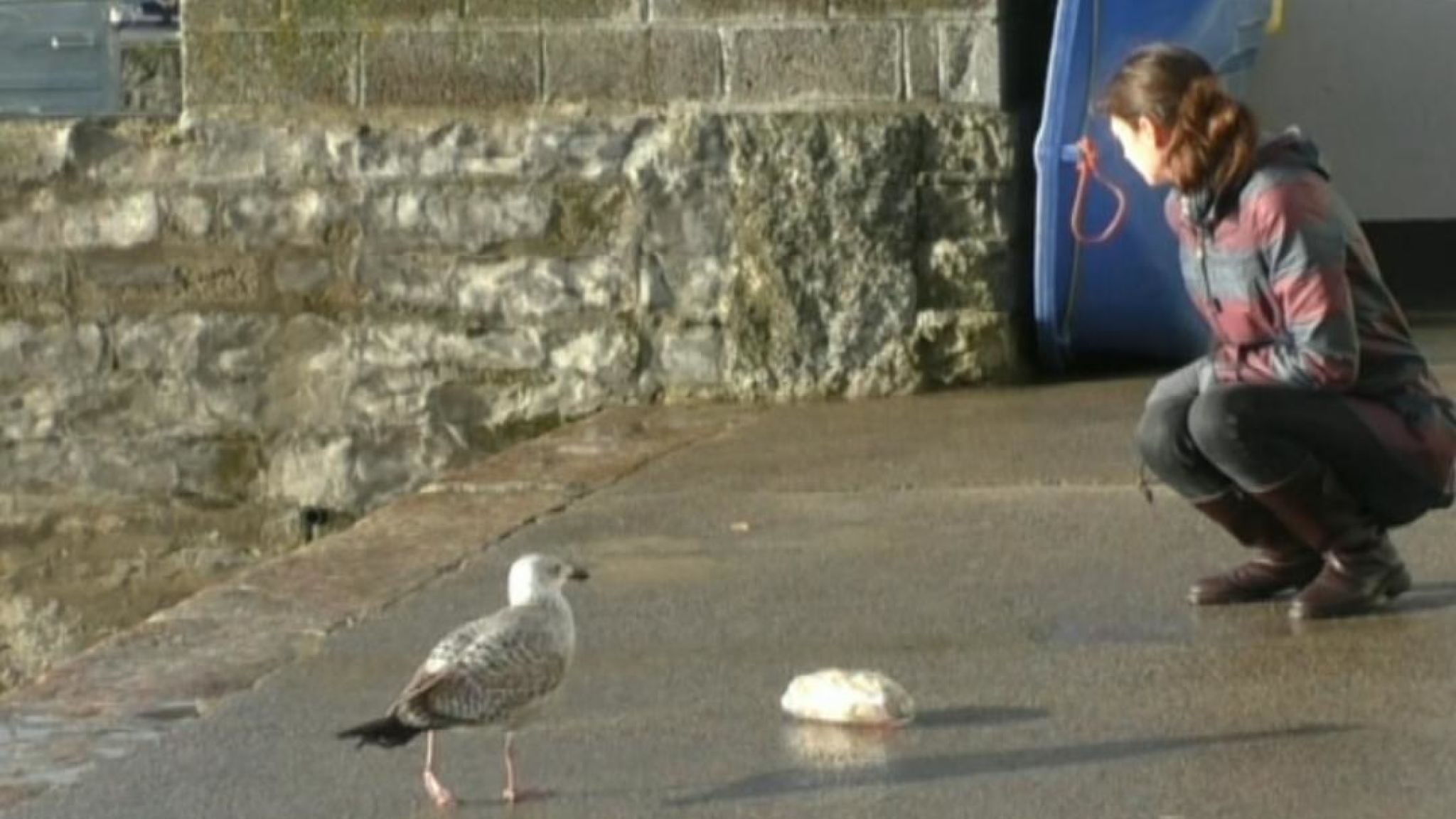
In the Looking Away treatment, the experimenter turned her head and eyes approximately 60° (randomly left or right) away from the gull and maintained this position until she heard the gull peck at the food bag.

gulls = read.delim("https://raw.githubusercontent.com/uopsych/psy611/refs/heads/master/data/gulls/pairs.txt")
gulls

   GullID  At Away
1   FAL01 210   35
2   FAL03 300   80
3   FAL04   6    3
4   PEN03  18   21
5   W120M  47   13
6    W019  25    4
7   PNZ01   4   13
8   PNZ02   9    8
9   STI01 300   18
10  STI02 300    6
11   W186  11    8
12  STI03   4    3
13  STI04   4    6
14  HEL02  12   19
15  NEW01 300    6
16  NEW02  63   16
17  NEW03 300  166
18  PER01  24   66
19  TRU01 300  167

FAL = Falmouth PEN = Penryn

Hypothesis testing

Use a paired-samples t-test because we have the same gulls in both conditions.

\(\large H_0\): There is no difference in how long it takes gulls to approach food between conditions.

\(\large H_1\): Gulls take longer to approach food in one of the conditions.

Sampling distribution

t-distribution requires two parameters, a mean and a standard deviation.

The mean of our sampling distribution comes from our null hypothesis, so

\[\large \mu = 0\]

Sampling distribution

Our standard deviation of our sampling distribution is the standard error of difference scores. This is calculated via the following steps

1. calculating difference scores \((X_{1i}-X_{2i} = D_i)\)
2. calculating the standard deviation of the difference scores \((s_D = \hat{\sigma}_D)\), and
3. dividing the standard deviation by the square root of the number of pairs in your study \((se_D = \frac{\hat{\sigma}_D}{\sqrt{N}})\).

(difference = gulls$At - gulls$Away)

 [1] 175 220   3  -3  34  21  -9   1 282 294   3   1  -2  -7 294  47 134 -42 133

We can take the mean of this new variable:

(m_delta = mean(difference))

[1] 83.10526

And we can calculate the standard deviation

(s_delta = sd(difference))

[1] 115.8485

To calculate the standard error of difference scores, we simply divide the standard deviation by the square root of the number of pairs or, if repeated measures, the number of subjects.

(se_delta = s_delta/sqrt(nrow(gulls)))

[1] 26.57747

\[\frac{\hat{\sigma}_\Delta}{\sqrt{N}} = \frac{115.85}{\sqrt{19}} = 26.58\]

df = nrow(gulls)-1
cv_t = qt(df = df, p = .975)
t_x = seq(-3.76, 3.76)
plot_t = data.frame(t_x) %>%
  ggplot(aes(x=t_x)) +
  stat_function(fun = function(x) dt(x, df), geom = "line") +
  stat_function(fun = function(x) dt(x, df), geom = "area", 
                xlim = c(cv_t, 3.76), fill = "purple") +
  stat_function(fun = function(x) dt(x, df), geom = "area", 
                xlim = c(-3.76, -1*cv_t), fill = "purple") +
  labs(title = "Sampling distribution \n(in t)", y = "density", x = "t")+
  theme_pubr(base_size = 20)

cv_x = cv_t*se_delta 
x = t_x*se_delta
plot_x = data.frame(x) %>%
  ggplot(aes(x=x)) +
  stat_function(fun = function(x) dt(x = x/se_delta, df = df), geom = "line") +
  stat_function(fun = function(x) dt(x/se_delta, df = df), geom = "area", 
                xlim = c(cv_x, max(x)), fill = "purple") +
  stat_function(fun = function(x) dt(x/se_delta, df = df), geom = "area", 
                xlim = c(min(x), -1*cv_x), fill = "purple") +
  labs(title = "Sampling distribution \n(in difference in seconds)", y = "density", x = "difference seconds")+
  theme_pubr(base_size = 20)

ggarrange(plot_t, plot_x, ncol = 2)

Test statistic

\[t_{df = N-1} = \frac{\bar{\Delta}-\mu}{\frac{\hat{\sigma}_\Delta}{\sqrt{N}}}\]

In this case, N refers to the number of pairs, not the total sample size.

\[t_{df = N-1} = \frac{83.11-0}{26.58} = 3.13\]

Note: A paired-samples t-test is exactly the same as a one-sample t-test on the difference scores.

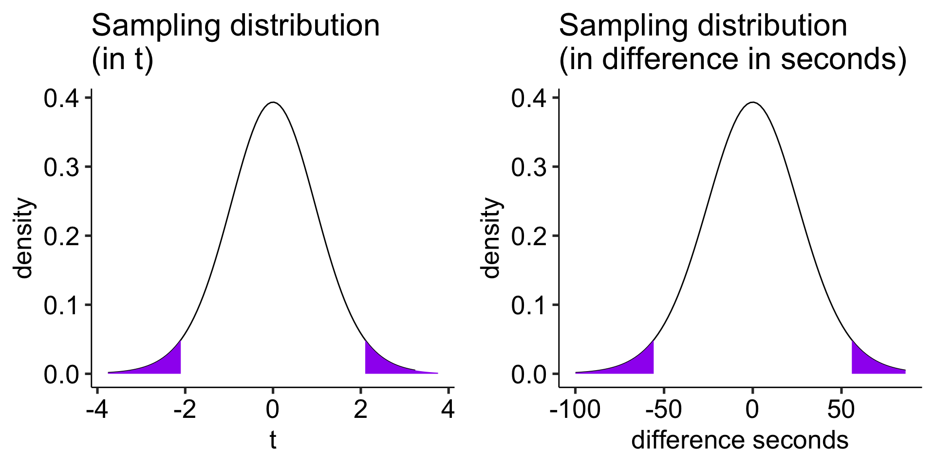
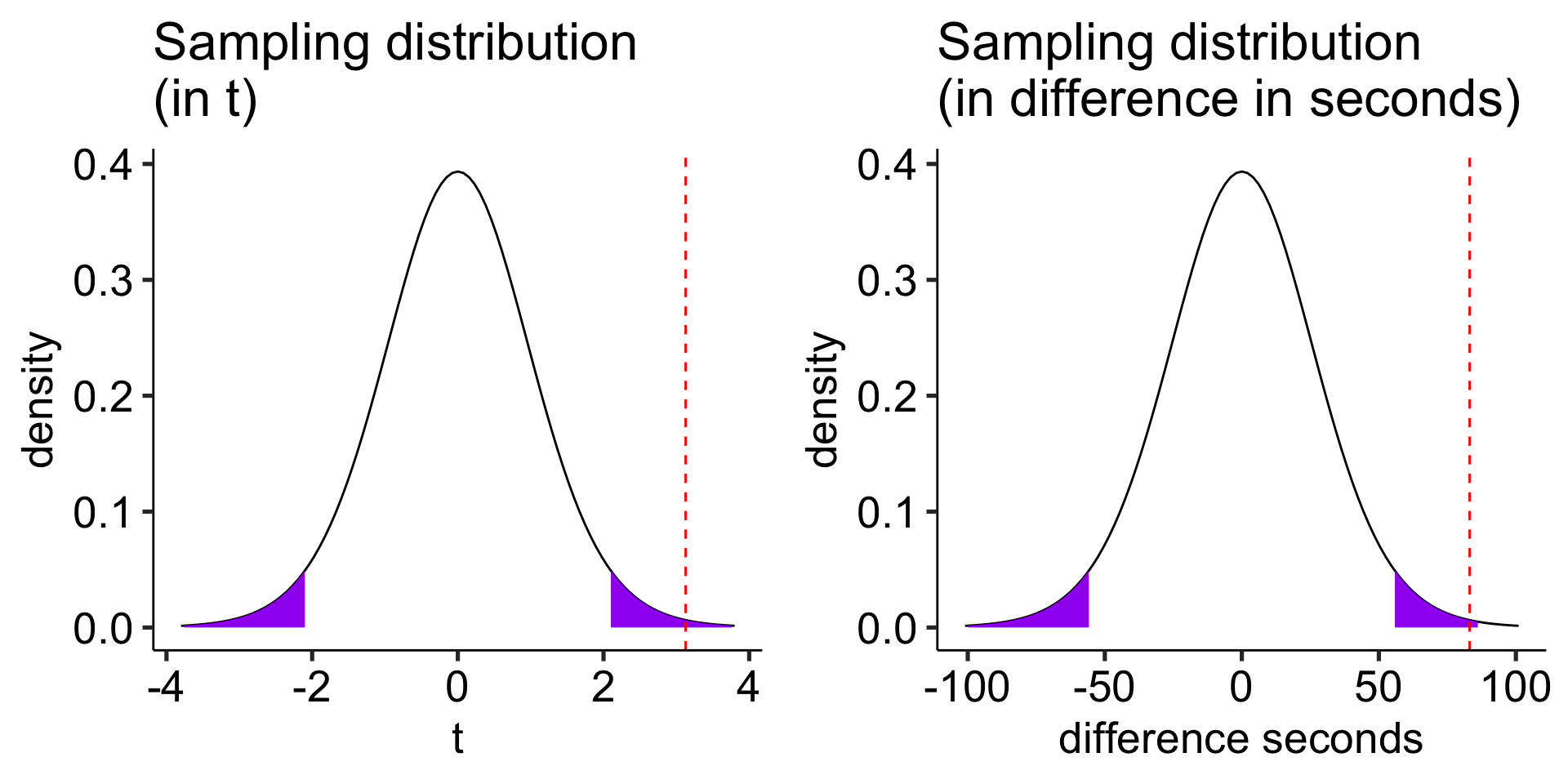
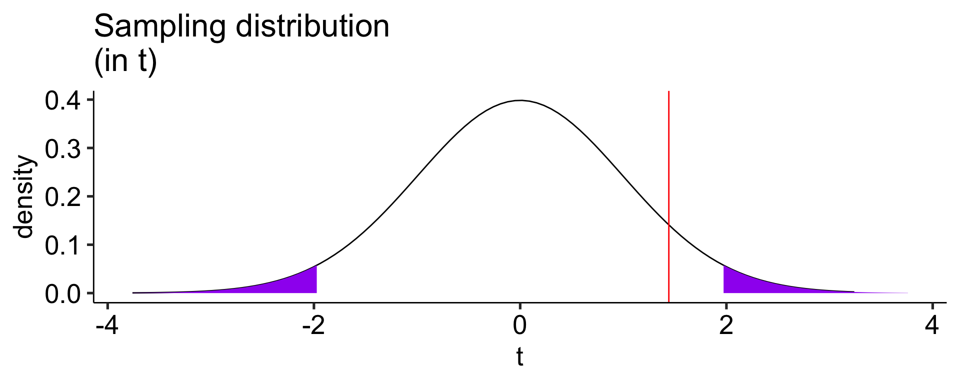
df = nrow(gulls)-1
cv_t = qt(df = df, p = .975)
t_x = seq(-3.76, 3.76)
statistic_t = m_delta/se_delta
plot_t = data.frame(t_x) %>%
  ggplot(aes(x=t_x)) +
  stat_function(fun = function(x) dt(x, df), geom = "line") +
  stat_function(fun = function(x) dt(x, df), geom = "area", 
                xlim = c(cv_t, 3.76), fill = "purple") +
  stat_function(fun = function(x) dt(x, df), geom = "area", 
                xlim = c(-3.76, -1*cv_t), fill = "purple") +
  geom_vline(aes(xintercept = statistic_t), linetype = 2, color = "red")+
  labs(title = "Sampling distribution \n(in t)", y = "density", x = "t")+
  scale_x_continuous(limits = c(-3.8, 3.8))+
  theme_pubr(base_size = 20)

cv_x = cv_t*se_delta 
x = t_x*se_delta
statistic_x = statistic_t*se_delta
plot_x = data.frame(x) %>%
  ggplot(aes(x=x)) +
  stat_function(fun = function(x) dt(x = x/se_delta, df = df), geom = "line") +
  stat_function(fun = function(x) dt(x/se_delta, df = df), geom = "area", 
                xlim = c(cv_x, max(x)), fill = "purple") +
  stat_function(fun = function(x) dt(x/se_delta, df = df), geom = "area", 
                xlim = c(min(x), -1*cv_x), fill = "purple") +
  geom_vline(aes(xintercept = statistic_x), linetype = 2, color = "red")+
  labs(title = "Sampling distribution \n(in difference in seconds)", y = "density", x = "difference seconds")+
  scale_x_continuous(limits = c(-3.8*se_delta, 3.8*se_delta))+
  theme_pubr(base_size = 20)

ggarrange(plot_t, plot_x, ncol = 2)

Another option is to calculate the area above the absolute value of the test statistic and multiply that by two – this estimates the probability of finding this test statistic or more extreme.

(t_statistic = m_delta/se_delta)

[1] 3.126906

pt(t_statistic, df = 19-1, lower.tail = F)

[1] 0.002912942

pt(t_statistic, df = 19-1, lower.tail = F)*2

[1] 0.005825884

t-test functions

t.test(x = gulls$At, 
       y = gulls$Away, 
       paired = TRUE)

    Paired t-test

data:  gulls$At and gulls$Away
t = 3.1269, df = 18, p-value = 0.005826
alternative hypothesis: true mean difference is not equal to 0
95 percent confidence interval:
  27.26807 138.94246
sample estimates:
mean difference 
       83.10526 

t-test functions

lsr::pairedSamplesTTest(formula = ~Away + At, data = gulls)

   Paired samples t-test 

Variables:  Away , At 

Descriptive statistics: 
              Away      At difference
   mean     34.632 117.737    -83.105
   std dev. 50.897 135.166    115.849

Hypotheses: 
   null:        population means equal for both measurements
   alternative: different population means for each measurement

Test results: 
   t-statistic:  -3.127 
   degrees of freedom:  18 
   p-value:  0.006 

Other information: 
   two-sided 95% confidence interval:  [-138.942, -27.268] 
   estimated effect size (Cohen's d):  0.717 

Example 2: Larks and Owls

People differ in their optimal time of day to perform a task (morning people = larks, evening people = owls). One study tested whether mind-wandering was more likely at one time of day and as a function of chronotype. Participants completed an attention task twice: once in the morning and once in the evening.

For this example, we’ll be ignoring individual differences (weep) and focus only on the mind-wandering task variable.

lao = read.csv("https://raw.githubusercontent.com/uopsych/psy611/refs/heads/master/data/Larks%20and%20Owls.csv")

lao %>% select(Subject, TimeOfDay, MWCount) %>% head()

  Subject TimeOfDay MWCount
1       1   Evening      15
2       1   Morning       5
3       2   Morning      11
4       2   Evening      13
5       3   Evening      29
6       3   Morning      26

lsr::pairedSamplesTTest(formula = MWCount~TimeOfDay, data = lao, id = "Subject")

   Paired samples t-test 

Outcome variable:   MWCount 
Grouping variable:  TimeOfDay 
ID variable:        Subject 

Descriptive statistics: 
            Evening Morning difference
   mean      19.692  21.431     -1.738
   std dev.   8.827   9.545      8.486

Hypotheses: 
   null:        population means equal for both measurements
   alternative: different population means for each measurement

Test results: 
   t-statistic:  -2.336 
   degrees of freedom:  129 
   p-value:  0.021 

Other information: 
   two-sided 95% confidence interval:  [-3.211, -0.266] 
   estimated effect size (Cohen's d):  0.205 

Visualizing this test

What is important to convey in a visualization of these data?

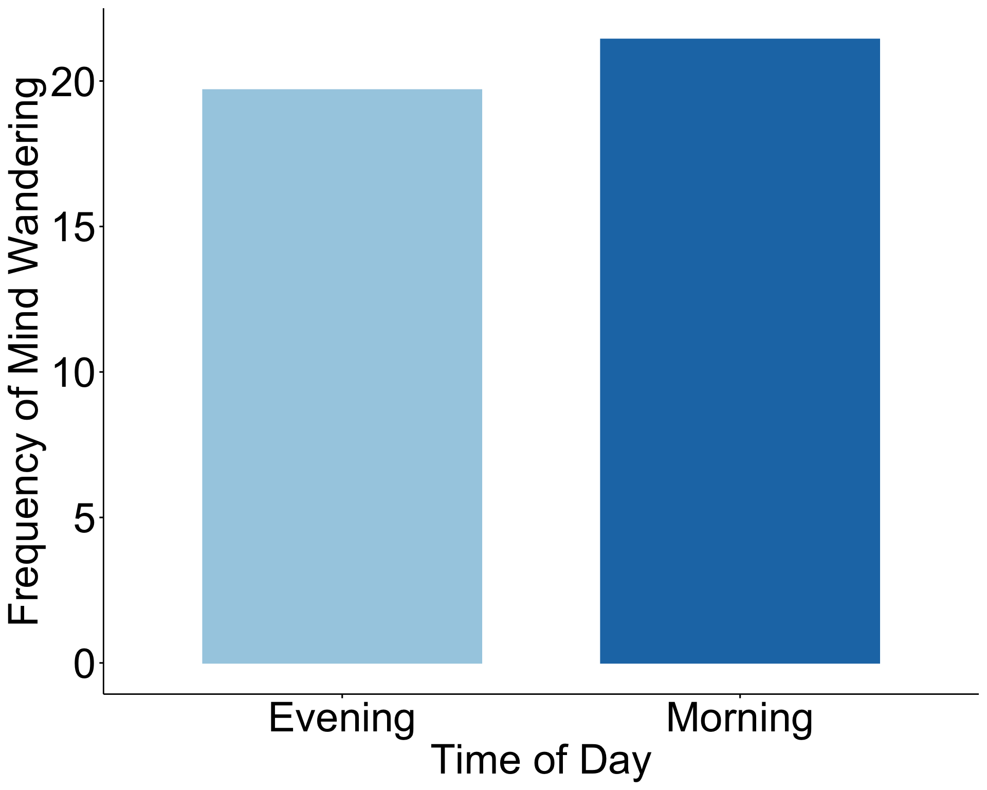
• The most obvious piece of information are means. (This is a test of the difference of means).
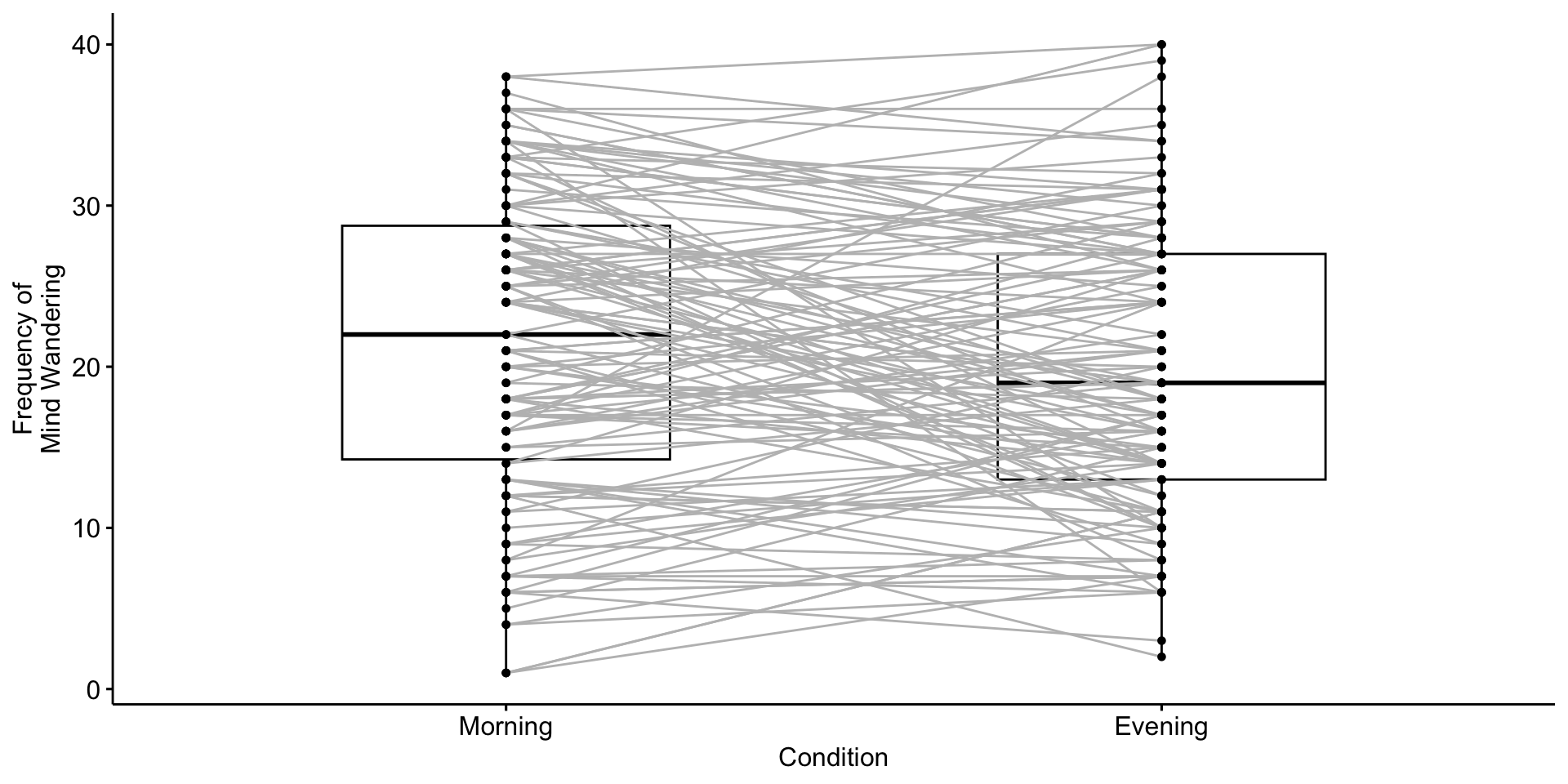
• Why is this a bad plot?

ggpubr::ggbarplot(data = lao,
                    x = "TimeOfDay", 
                    y = "MWCount", 
                    add = "mean", 
                    fill = "TimeOfDay",
                    color = "TimeOfDay",
                    palette = "Paired", 
                    xlab = "Time of Day",
                    ylab = "Frequency of Mind Wandering") +
  rremove("legend") +
  theme(
    axis.title = element_text(size = 30),
    axis.text = element_text(size = 30))

Viz: show the mean tested

lao_wide = lao %>% 
  select(Subject, TimeOfDay, MWCount) %>% 
  pivot_wider(names_from = TimeOfDay, values_from = MWCount) %>% 
  mutate(diff = Evening-Morning) 

se = sd(lao_wide$diff)/sqrt(nrow(lao_wide))
moe = se*qt(p = .975, df = nrow(lao_wide) - 1)
lower_ci = mean(lao_wide$diff) - moe
upper_ci = mean(lao_wide$diff) + moe

lao_wide %>% 
  ggplot(aes(x = diff)) +
  geom_rect(aes(xmin = lower_ci,
                xmax = upper_ci,
                ymin = -Inf,
                ymax = Inf),
            fill = "#85D4C8") +
  geom_histogram(fill = "grey70",
                 color = "black") +
  geom_vline(
    aes(xintercept = mean(diff)),
    linetype = "dashed") +
  labs(
    x = "Difference in Mind Wandering",
    y = "Count"
  ) +
  theme_minimal()

Viz: show the individual people

ggpubr::ggpaired(data = lao_wide, 
                 cond1 = "Morning", 
                 cond2 = "Evening", 
                 line.color = "grey",
                 ylab = "Frequency of\nMind Wandering")

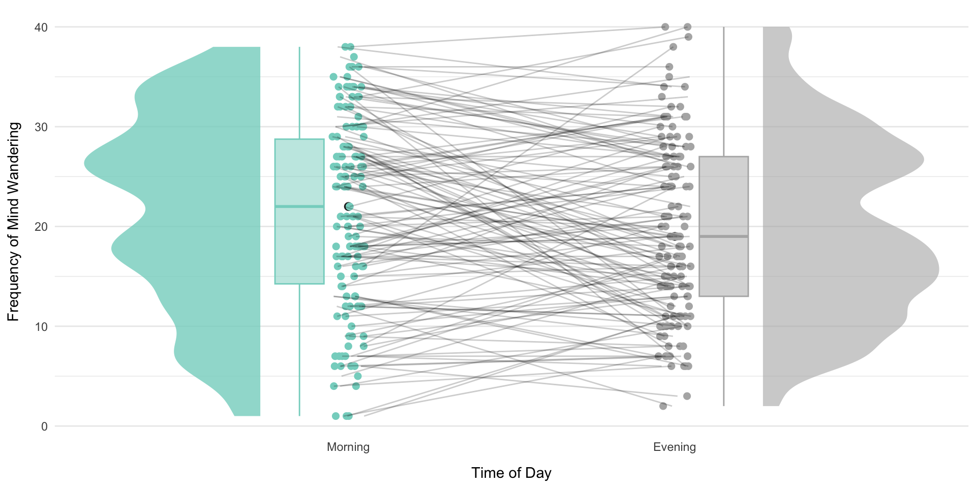
library(ggdist)
library(gghalves)

#without this line of code, R will organize things alphabetically.
# but i think it makes more sense for morning to come first
lao$TimeOfDay = factor(lao$TimeOfDay, levels = c("Morning", "Evening"))

# Create plot
ggplot(lao, aes(x = TimeOfDay, y = MWCount)) +
  # Add violin plots on opposite sides
  stat_halfeye(
    data = subset(lao, TimeOfDay == "Morning"),
    adjust = 0.5,
    width = 0.6,
    justification = 1.5,
    .width = 0,
    fill = "#85D4C8",
    alpha = 0.8,
    side = "left"
  ) +
  stat_halfeye(
    data = subset(lao, TimeOfDay == "Evening"),
    adjust = 0.5,
    width = 0.6,
    justification = -0.5,
    .width = 0,
    fill = "grey70",
    alpha = 0.6
  ) +
  # Add boxplots
  geom_boxplot(
    data = subset(lao, TimeOfDay == "Morning"),
    aes(fill = TimeOfDay, color = TimeOfDay),
    position = position_nudge(x = -.15),
    width = 0.15,
    outlier.shape = NA,
    alpha = 0.5
  ) +
  geom_boxplot(
    data = subset(lao, TimeOfDay == "Evening"),
    aes(fill = TimeOfDay, color = TimeOfDay),
    position = position_nudge(x = .15),
    width = 0.15,
    outlier.shape = NA,
    alpha = 0.5
  ) +
  # Add points and lines
  geom_point(aes(group = Subject, color = TimeOfDay),
             size = 2,
             position = position_jitter(width = 0.05, height = 0, seed = 123)) +
  geom_line(aes(group = Subject),
            position = position_jitter(width = 0.05, height = 0, seed = 123),
            alpha = 0.2) +
  # Customize theme
  scale_fill_manual(values = c("#85D4C8", "grey70")) +
  scale_color_manual(values = c("#85D4C8", "grey70")) +
  theme_minimal() +
  theme(
    panel.grid.major.x = element_blank(),
    panel.grid.minor.x = element_blank(),
    axis.title.x = element_text(margin = margin(t = 10)),
    axis.title.y = element_text(margin = margin(r = 10))
  ) +
  labs(
    x = "Time of Day",
    y = "Frequency of Mind Wandering"
  ) +
  guides(
    fill = "none",
    color = "none"
  )

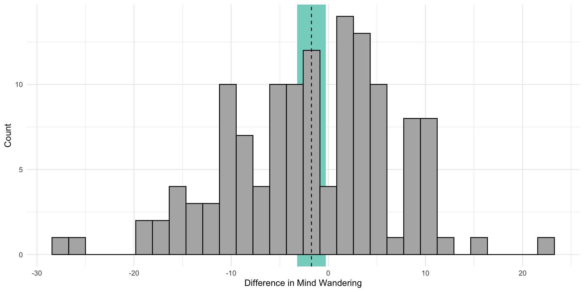
Visualizing paired-samples t-test

There’s a choice between displaying the statistics being tested (the mean and standard error of the difference scores) and displaying the data in its original units (two points per subject, means of individual conditions). You can’t have both. Pick the one that best conveys the information you want a reader to walk away with.

Better yet, put one in your manuscript and the other in supplemental material!

Also, making good data visualizations can take some work. But it’s really worth it. This is where AI can be a great friend!

The variance of difference scores

With the raw data, the calculation of the variance of the standard deviation scores \(\large (\hat{\sigma}_\Delta)\) is intuitive. Sometimes you will not have access to the raw data, but will want to conduct the test.

For example, you read a study that compares a sample of Oregon students to known US benchmarks on several variables using multiple one-sample t-tests; you want to know whether OR students respond more to one variable than the other.

school = read_csv(here("data/census_at_school.csv"))
school = school %>% filter(ClassGrade >= 9) %>%
  filter(!is.na(Importance_reducing_pollution)) %>%
  filter(!is.na(Importance_recycling_rubbish)) 
psych::describe(school[,c("Importance_reducing_pollution", "Importance_recycling_rubbish")], fast = T) %>%
  select(n, mean, sd) %>%
  kable(., col.names = c("N", "Mean", "SD"),
        digits = 2) %>%
  kable_styling()

	N	Mean	SD
Importance_reducing_pollution	194	792.15	937.03
Importance_recycling_rubbish	194	714.85	652.65

cor_12 = cor(school$Importance_reducing_pollution, 
             school$Importance_recycling_rubbish, 
             use = "pairwise")

The correlation between these variables is 0.61.

It turns out that the mean difference score is the same as the difference in means, so that’s an easy part of the calculation.

But the calculation of the standard deviation becomes a little more complicated:

\[\large \hat{\sigma}_\Delta = \sqrt{\hat{\sigma}^2_{X_1} + \hat{\sigma}^2_{X_2} - 2r(\hat{\sigma}_{X_1}\hat{\sigma}_{X_2})}\]

sd_1 = 937.03
sd_2 = 652.65
cor_12 = .61
var_d = sd_1^2 + sd_2^2 -2*cor_12*sd_1*sd_2
sqrt(var_d)

[1] 746.9157

Now you have all the information you need for the statistical test!

(t = (792.15-714.85)/(746.92/sqrt(194)))

[1] 1.441472

pt(t, df = 193, lower.tail = F)*2

[1] 0.1510719

Useful for meta-analysis or getting more information from articles you read.

What else can this equation tell us?

What happens if the two variables are highly correlated with each other?

\[\large \hat{\sigma}_\Delta = \sqrt{\hat{\sigma}^2_{X_1} + \hat{\sigma}^2_{X_2} - 2r(\hat{\sigma}_{X_1}\hat{\sigma}_{X_2})}\]

• What happens if \(\large r\) is large and positive?

• What happens if \(\large r\) is small and positive?

• What happens if \(\large r\) is negative?

large and postive: se is very small small and positive: se is smaller but not so much negative: se is bigger

take away: likely to find differences when two measures are positively associated, but hurt if negatively may consider reverse scoring measures…

Assumptions

• Independence (between pairs)
• Normality

Note: These are the same assumptions as a one-sample t-test.

Next time…

Dealer’s choice!