Assumptions and Effect Sizes
Announcements
- Graded Quiz 9 will be returned tomorrow during lab.
- Next week, submit quiz corrections in my mailbox (Straub front office).
Last time
Introduction to independent samples t-tests
Standard error of the difference of means
Pooled variance, \(\hat{\sigma}_P\)
Confidence intervals around the difference in means
Confidence intervals around different means
Review of independent samples t-tests
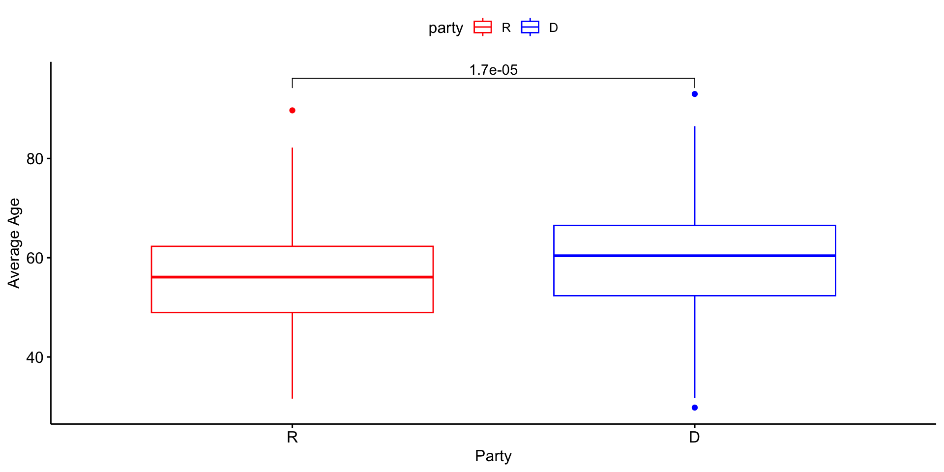
It’s generally argued that Republicans have an age problem – but are they substantially older than Democrats?
In 2014 (midterm election before the most recent presidential election), Five Thirty Eight did an analysis of the ages of elected members of Congress. They’ve provided their data, so we can run analyses on our own.
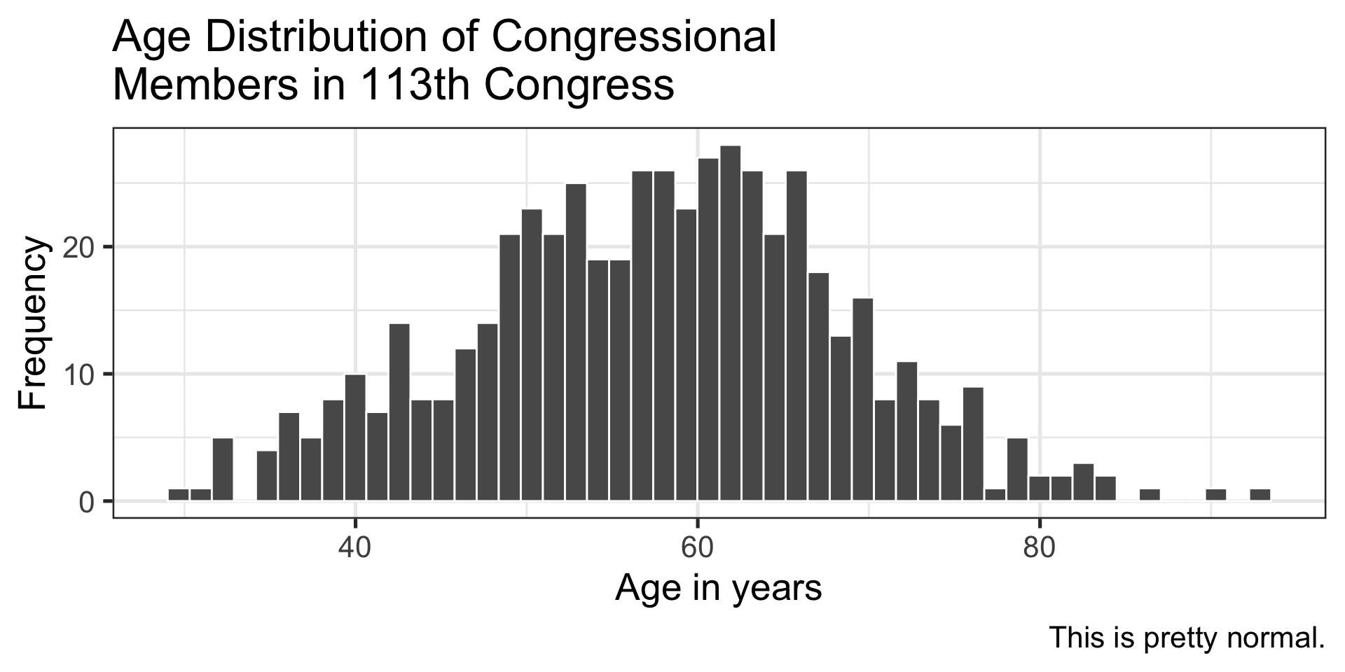
Code
congress %>% ggplot(aes(x = age, fill = party)) + geom_histogram(bins = 50, color = "white", position = "dodge") + labs(x = "Age in years", y = "Frequency", title = "Age Distribution of Congressional \nMembers in 113th Congress", caption = "This is pretty normal.") + scale_fill_manual(values = c("blue", "red")) + theme_bw(base_size = 20)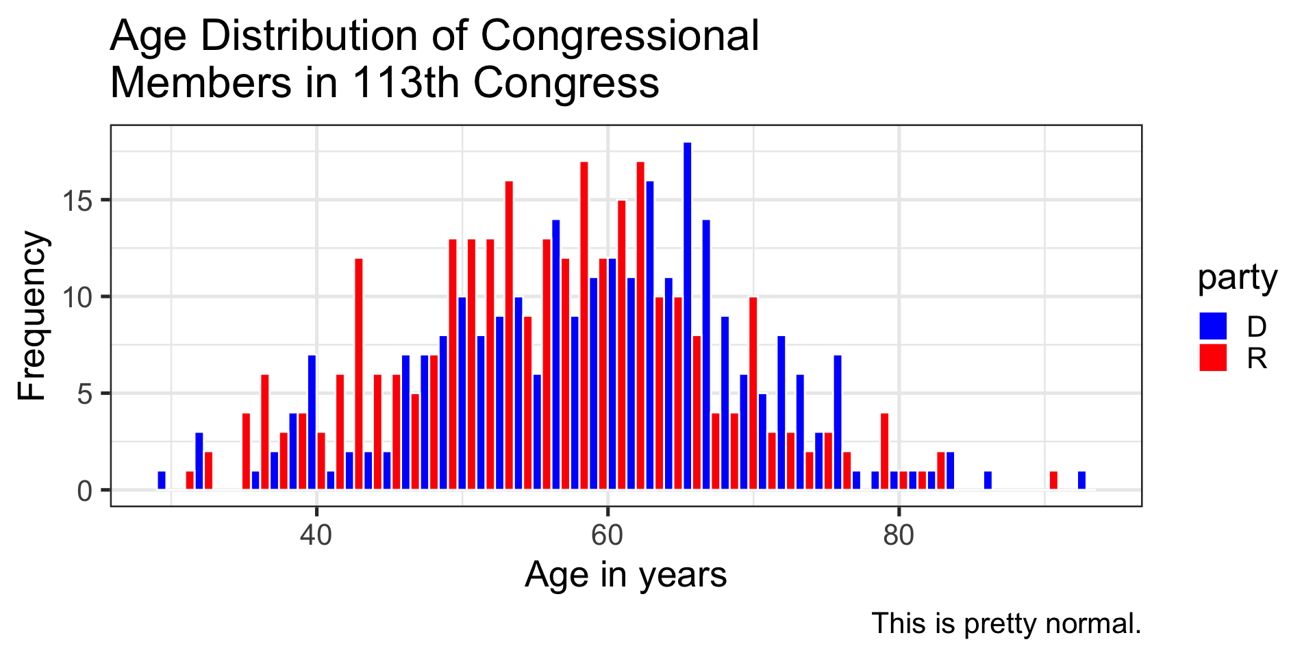
Descriptive statistics by group
group: D
vars n mean sd median min max range skew kurtosis se
X1 1 259 59.55 10.85 60.4 29.8 93 63.2 -0.19 0.02 0.67
------------------------------------------------------------
group: R
vars n mean sd median min max range skew kurtosis se
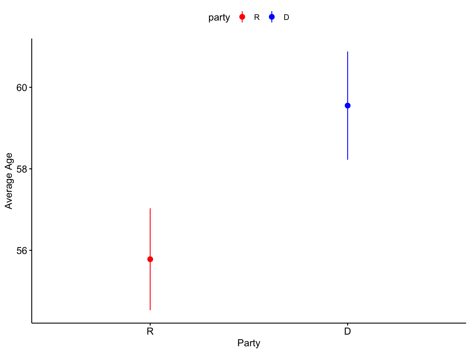
X1 1 283 55.78 10.68 56.1 31.6 89.7 58.1 0.13 -0.11 0.64\[ \bar{X}_1 = 59.55 \] \[ \hat{\sigma}_1 = 10.85 \] \[ N_1 = 259 \]
\[ \bar{X}_2 = 55.78 \] \[ \hat{\sigma}_2 = 10.68 \] \[ N_2 = 283 \]
Next we build the sampling distribution under the null hypotheses.
\[ \mu = 0 \\\] \[\sigma_D = \sqrt{\frac{(259-1){10.85}^2 + (283-1){10.68}^2}{259+283-2}} \sqrt{\frac{1}{259} + \frac{1}{283}}\] \[= 10.76\sqrt{\frac{1}{259} + \frac{1}{283}} = 0.93\] \[df = 540\] ————————————————————————
Code
x = c(-5:5)

data.frame(x) %>%
  ggplot(aes(x=x)) +
  stat_function(fun= function(x) dt(x, df = df), geom = "area",
                xlim = c(cv, 5), fill = "purple") +
  stat_function(fun= function(x) dt(x, df = df), geom = "area",
                xlim = c(-5, cv*-1), fill = "purple") +
  stat_function(fun= function(x) dt(x, df = df), geom = "line") +
  geom_vline(aes(xintercept = t), color = "black")+
  labs(x = "Difference in means", y = "density") +
  theme_light(base_size = 20)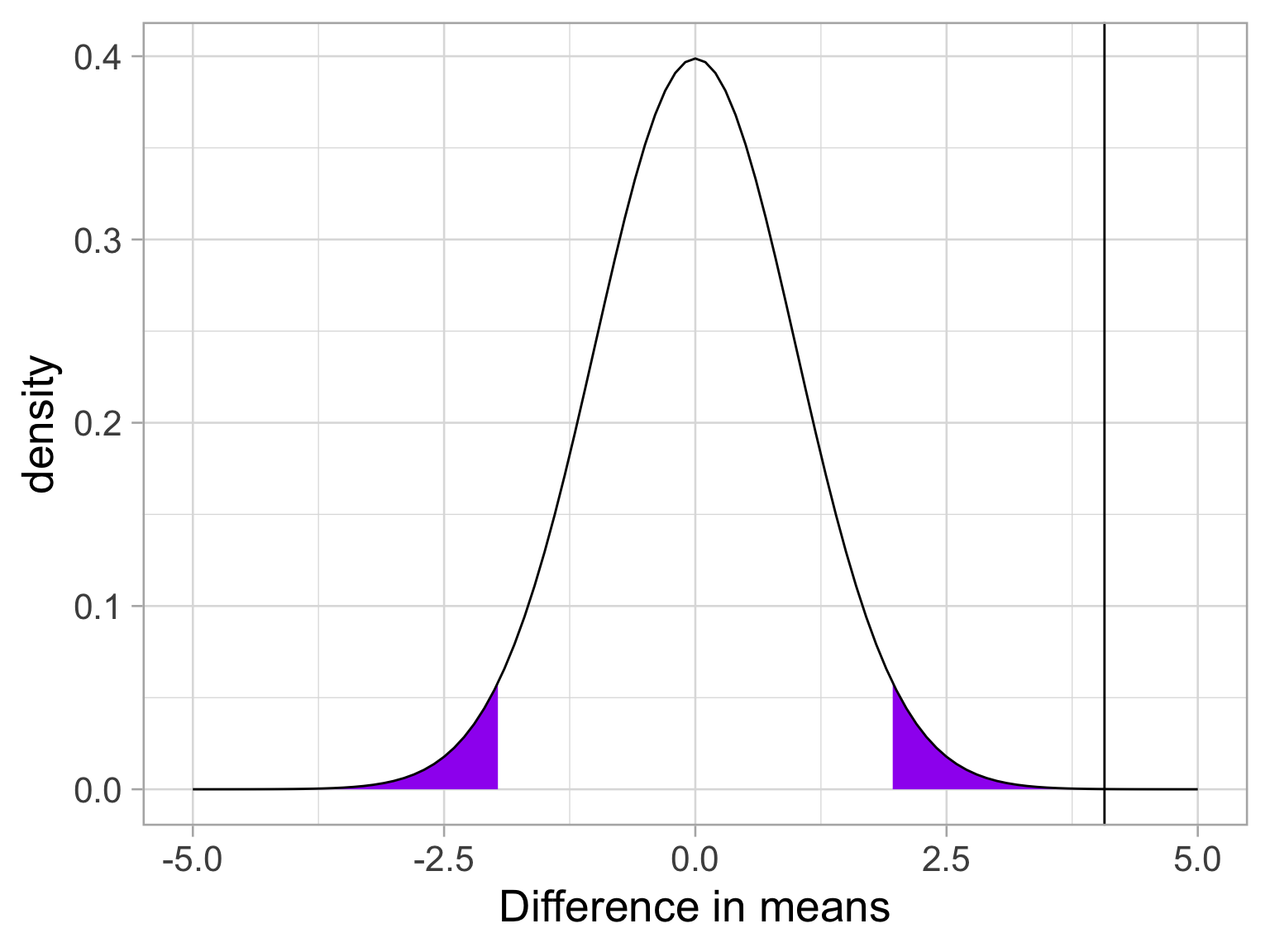
Effect sizes
Cohen suggested one of the most common effect size estimates—the standardized mean difference—useful when comparing a group mean to a population mean or two group means to each other. This is referred to as Cohen’s d.
\[\delta = \frac{\mu_1 - \mu_0}{\sigma} \approx d = \frac{\bar{X}_1-\bar{X}_2}{\hat{\sigma}_p}\]
Cohen’s d is in the standard deviation (Z) metric.
What happens to Cohen’s d as sample size gets larger?
Let’s go back to our politics example:
Democrats
\[\small \bar{X}_1 = 59.55 \] \[\small \hat{\sigma}_1 = 10.85 \] \[\small N_1 = 259 \]
Republicans \[\small \bar{X}_2 = 55.78 \] \[\small \hat{\sigma}_2 = 10.68 \] \[\small N_2 = 283 \]
Let’s go back to our politics example:
\[\hat{\sigma}_p = \sqrt{\frac{(259-1){10.85}^2 + (283-1){10.68}^2}{259+283-2}} = 10.76\]
\[d = \frac{59.55-55.78}{10.76} = 0.35\]
How do we interpret this? Is this a large effect?
Cohen1 suggests the following guidelines for interpreting the size of d:
- .2 = Small
- .5 = Medium
- .8 = Large
An aside, to calculate Cohen’s D for a one-sample t-test: \[d = \frac{\bar{X}-\mu}{\hat{\sigma}}\]
Cohen’s D (Paired-samples t)
Recall our gull example from the paired-samples t-test lecture. The average difference in seconds was \(83.11 (SD = 115.85)\).
Calculating a standardized effect size for a paired samples t-test (and research design that includes nesting or dependency) is slightly complicated, because there are two levels at which you can describe results.
The first level is the within-subject (or within-pair, or within-gull) level, and this communicates effect size in the unit of differences (of units).
\[d = \frac{\bar{\Delta}}{\hat{\sigma_\Delta}} = \frac{83.11}{115.85} = 0.72\]
The interpretation is that, on average, variability within a single gull is about .72 standard deviations of differences of seconds.
Cohen’s D (Paired-samples t)
The second level is the between-conditions variance, which is in the units of your original outcome and communicates how the means of the two conditions differ.
For that, you can use the Cohen’s d calculated for independent samples t-tests.
Which one should you use?
The first thing to recognize is that, unlike hypothesis testing, there are no standards for effect sizes. When Cohen developed his formula in 1988, he never bothered to precisely define \(\large \sigma\). Interpretations have varied, but no single method for within-subjects designs has been identified.
Most often, textbooks will argue for the within-pairs version, because this mirrors the hypothesis test.
Which one should you use?
Some1 argue the between-conditions version is actually better because the paired-design is used to reduce noise by adjusting our calculation of the standard error. But that shouldn’t make our effect bigger, just easier to detect. The other argument is that using the same formula (the between-conditions version) allows us to compare effect sizes across many different designs, which are all trying to capture the same effect.
When you have meaningful units, also express the effect size in terms of those units. This is the most interpretable effect size available to you.
Democrats are, on average, 3.77 years older than Republicans.
Gulls take, on average, 83.11 seconds longer to approach chips when people stare at them than when people are looking away.
Assumptions: When can you not use Student’s t-test?
Recall the three assumptions of Student’s t-test:
- Independence
- Normality
- Homogeneity of variance
Assumptions: When can you not use Student’s t-test?
There are no good statistical tests to determine whether you’ve violated the assumption of independence – it depends on how you sampled your population.
- Draw phone numbers at random from a phone book?
- Recruit random sets of fraternal twins?
- Randomly select houses in a city and interview the person who answers the door?
Homogeneity of variance
Homogeneity of variance can be checked with Levene’s procedure. It tests the null hypothesis that the variances for two or more groups are equal (or within sampling variability of each other):
\[H_0: \sigma^2_1 = \sigma^2_2\]
Levene’s test can be expanded to more than two variances; in this case, the alternative hypothesis is that at least one variance is different from at least one other variance.
Levene’s produces a statistic, W, that is F distributed with degrees of freedom of \(k-1\) and \(N-k\).
Levene's Test for Homogeneity of Variance (center = "mean")
       Df F value Pr(>F)
group   1  0.0663  0.797
      540
Like other tests of significance, Levene’s test gets more powerful as sample size increases. So unless your two variances are exactly equal to each other (and if they are, you don’t need to do a test), your test will be “significant” with a large enough sample. Part of the analysis has to be an eyeball test – is this “significant” because they are truly different, or because I have many subjects.
Homogeneity of variance
The homogeneity assumption is often the hardest to justify, empirically or conceptually. If we suspect the means for the two groups could be different (H1), that might extend to their variances as well.
Treatments that alter the means for the groups could also alter the variances for the groups.
Welch’s t-test removes the homogeneity requirement, but uses a different calculation for the standard error of the mean difference and the degrees of freedom. One way to think about the Welch test is that it is a penalized t-test, with the penalty imposed on the degrees of freedom in relation to violation of variance homogeneity (and differences in sample size).
Welch’s t-test
\[t = \frac{\bar{X}_1-\bar{X_2}}{\sqrt{\frac{\hat{\sigma}^2_1}{N_1}+\frac{\hat{\sigma}^2_2}{N_2}}}\]
So that’s a bit different – the main difference here is the way that we weight sample variances. It’s true that larger samples still get more weight, but not as much as in Student’s version. Also, we divide variances here by N instead of N-1, making our standard error larger.
Welch’s t-test
The degrees of freedom are different:
\[df = \frac{[\frac{\hat{\sigma}^2_1}{N_1}+\frac{\hat{\sigma}^2_2}{N_2}]^2}{\frac{[\frac{\hat{\sigma}^2_1}{N1}]^2}{N_1-1}+\frac{[\frac{\hat{\sigma}^2_2}{N2}]^2}{N_2-1}}\]
These degrees of freedom can be fractional. As the sample variances converge to equality, these df approach those for Student’s t, for equal N.
    Welch Two Sample t-test

data:  age by party
t = 4.0688, df = 534.2, p-value = 5.439e-05
alternative hypothesis: true difference in means between group D and group R is not equal to 0
95 percent confidence interval:
 1.949133 5.588133
sample estimates:
mean in group D mean in group R
       59.55097        55.78233
Normality
Finally, there’s the assumption of normality. Specifically, this is the assumption that the population is normal – if the population is normal, then our sampling distribution is definitely normal and we can use a t-distribution.
But even if the population is not normal, the CLT lets us assume our sampling distribution is normal because as N approaches infinity, the sampling distributions approaches normality. So we can be pretty sure the sampling distribution is normal.
Normality
One thing we can check – the only distribution we actually have access to – is the sample distribution. If this is normal, then we might guess that our population distribution is normal, and thus our sampling distribution is normal too.
Normality can be checked with a formal test: the Shapiro-Wilk test. The test statistic, W, has an expected value of 1 under the null hypothesis. Departures from normality reduce the size of W. A statistically significant W is a signal that the sample distribution departs significantly from normal.
Normality
But…
- With large samples, even trivial departures will be statistically significant.
- With large samples, the sampling distribution of the mean(s) will approach normality, unless the data are very non-normally distributed.
- Visual inspection of the data can confirm if the latter is a problem.
- Visual inspection can also identify outliers that might influence the data.
    Shapiro-Wilk normality test

data:  congress$age
W = 0.99663, p-value = 0.3168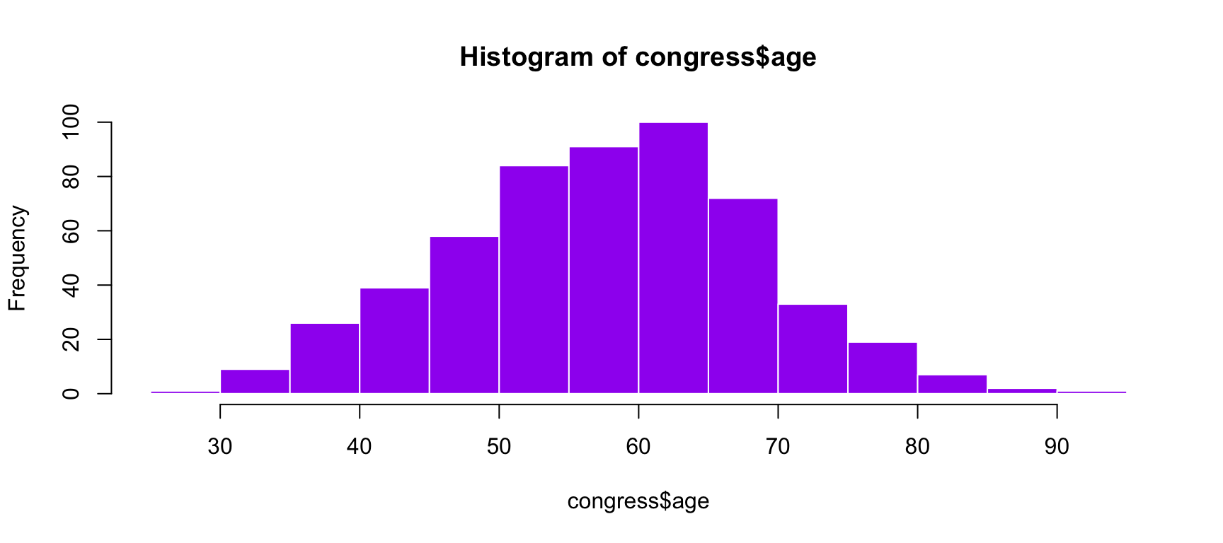
Bootstrapping
Imagine you had a sample of 6 people: Rachel, Monica, Phoebe, Joey, Chandler, and Ross. To bootstrap their heights, you would draw from this group many samples of 6 people with replacement, each time calculating the average height of the sample.
[1] "Monica" "Rachel" "Monica" "Phoebe" "Chandler" "Monica" [1] 66.66667[1] "Phoebe" "Joey" "Chandler" "Phoebe" "Rachel" "Joey" [1] 68.83333[1] "Phoebe" "Rachel" "Phoebe" "Rachel" "Phoebe" "Phoebe"[1] 67[1] "Monica" "Ross" "Rachel" "Ross" "Monica" "Phoebe"[1] 68.16667[1] "Phoebe" "Chandler" "Monica" "Phoebe" "Phoebe" "Rachel" [1] 67.66667[1] "Chandler" "Chandler" "Monica" "Rachel" "Chandler" "Phoebe" [1] 69[1] "Ross" "Monica" "Joey" "Chandler" "Rachel" "Chandler"[1] 69.5[1] "Rachel" "Phoebe" "Monica" "Chandler" "Joey" "Rachel" [1] 67.5 Rachel Monica Phoebe Joey Chandler Ross
65 65 68 70 72 73 [1] 68.16667 66.66667 68.00000 68.00000 68.33333 71.66667 68.33333 68.83333
[9] 66.83333 69.83333 67.66667 69.83333 69.33333 69.50000 67.83333 68.16667
[17] 70.33333 69.00000 70.00000 68.66667 68.50000 70.16667 68.00000 66.66667
[25] 68.33333 67.50000 69.33333 66.50000 68.50000 66.33333 69.33333 68.33333
[33] 69.33333 68.33333 66.33333 65.83333 67.33333 69.33333 66.00000 68.83333
[41] 69.83333 69.66667 70.00000 67.66667 68.50000 69.83333 66.83333 69.16667
[49] 67.83333 67.50000 67.16667 70.00000 68.16667 66.66667 69.66667 66.83333
[57] 68.83333 71.83333 68.16667 70.66667 69.66667 69.33333 68.66667 68.33333
[65] 66.66667 69.16667 69.50000 65.50000 68.83333 65.00000 69.83333 67.16667
[73] 69.83333 69.83333 71.16667 68.33333 69.50000 66.66667 67.16667 68.16667
[81] 67.50000 67.50000 69.16667 67.50000 68.00000 68.33333 68.83333 70.00000
[89] 68.50000 68.00000 68.83333 72.83333 67.33333 67.83333 69.66667 68.66667
[97] 69.66667 69.83333 68.50000 70.16667 72.00000 71.33333 68.50000 68.50000
[105] 67.50000 68.00000 69.16667 69.83333 69.33333 67.50000 70.66667 71.16667
[113] 68.83333 69.66667 66.83333 68.66667 69.33333 68.66667 69.33333 69.16667
[121] 68.00000 68.00000 69.50000 67.83333 69.00000 69.83333 67.00000 69.00000
[129] 70.16667 66.16667 66.16667 67.50000 70.00000 67.00000 69.33333 70.00000
[137] 68.16667 68.66667 68.00000 67.83333 68.83333 68.33333 69.66667 70.66667
[145] 68.00000 69.00000 67.50000 68.00000 68.66667 68.00000 70.00000 68.33333
[153] 69.33333 72.00000 69.00000 69.16667 70.16667 69.33333 68.33333 68.00000
[161] 67.33333 69.33333 68.00000 69.83333 70.50000 71.00000 67.50000 69.66667
[169] 69.66667 68.16667 66.83333 71.00000 68.00000 68.83333 68.83333 67.66667
[177] 70.16667 69.50000 68.16667 69.00000 67.33333 69.83333 68.66667 67.16667
[185] 69.16667 69.83333 71.33333 68.83333 68.66667 68.50000 69.83333 67.50000
[193] 68.66667 66.83333 69.16667 67.16667 67.66667 69.00000 68.00000 68.00000
[201] 70.33333 69.16667 68.66667 68.83333 68.83333 69.83333 69.50000 70.66667
[209] 68.33333 72.33333 68.83333 69.16667 68.83333 69.50000 68.50000 70.83333
[217] 70.33333 70.33333 67.50000 68.33333 69.50000 70.00000 71.00000 67.16667
[225] 67.50000 66.00000 66.83333 70.16667 68.33333 68.33333 68.66667 69.33333
[233] 66.33333 69.00000 67.83333 68.83333 65.50000 68.83333 67.33333 70.83333
[241] 69.50000 71.50000 70.00000 65.50000 68.33333 67.00000 69.00000 71.16667
[249] 66.50000 69.00000 65.83333 67.00000 68.16667 69.00000 65.50000 71.66667
[257] 71.66667 68.83333 67.16667 66.66667 68.83333 70.50000 70.83333 69.83333
[265] 67.83333 69.83333 71.66667 68.83333 71.00000 68.50000 70.00000 68.00000
[273] 70.33333 68.33333 68.83333 68.83333 69.50000 68.50000 68.66667 66.33333
[281] 67.16667 67.16667 68.83333 67.00000 70.00000 69.66667 68.50000 71.33333
[289] 70.50000 67.16667 69.83333 69.66667 69.33333 69.50000 69.00000 69.00000
[297] 70.83333 68.33333 68.00000 69.16667 70.33333 67.16667 70.50000 68.66667
[305] 69.00000 69.66667 69.16667 70.33333 69.33333 67.66667 68.50000 69.16667
[313] 70.33333 68.16667 68.83333 68.66667 68.33333 68.83333 68.00000 67.66667
[321] 67.83333 69.66667 69.33333 68.66667 70.66667 68.00000 69.00000 67.16667
[329] 67.83333 69.66667 69.83333 67.50000 68.50000 67.83333 68.33333 68.00000
[337] 67.50000 69.16667 70.50000 70.16667 68.33333 68.33333 68.00000 68.83333
[345] 69.33333 66.16667 67.33333 70.00000 65.83333 68.33333 69.33333 70.00000
[353] 68.33333 67.50000 69.66667 70.33333 68.33333 66.83333 68.50000 66.66667
[361] 69.83333 70.16667 67.50000 68.00000 69.00000 67.16667 68.66667 69.83333
[369] 69.16667 67.16667 68.16667 67.50000 68.83333 70.50000 69.33333 65.83333
[377] 68.00000 70.50000 67.66667 70.66667 68.33333 68.66667 69.66667 70.33333
[385] 67.50000 66.66667 67.33333 68.83333 67.50000 70.00000 69.33333 69.83333
[393] 70.50000 69.16667 69.00000 72.33333 69.00000 71.83333 69.16667 68.83333
[401] 68.00000 68.83333 67.66667 67.00000 67.83333 69.33333 70.33333 68.16667
[409] 67.66667 67.16667 67.33333 69.16667 68.00000 69.33333 67.83333 66.66667
[417] 67.83333 65.83333 68.66667 68.00000 70.66667 69.66667 68.33333 68.16667
[425] 67.83333 68.16667 67.16667 68.33333 68.50000 69.66667 69.00000 70.50000
[433] 67.66667 70.66667 69.00000 69.33333 68.33333 70.50000 66.00000 70.00000
[441] 69.33333 68.83333 67.33333 68.16667 68.83333 68.33333 68.00000 70.33333
[449] 70.00000 66.66667 70.50000 68.83333 69.33333 69.16667 69.16667 70.16667
[457] 70.66667 68.83333 70.83333 65.83333 68.50000 68.83333 68.83333 67.33333
[465] 69.50000 69.16667 68.83333 66.66667 66.50000 68.33333 68.16667 70.16667
[473] 69.83333 69.16667 67.50000 69.50000 68.33333 69.83333 69.16667 68.16667
[481] 70.66667 68.33333 68.83333 68.00000 70.16667 69.83333 69.00000 70.00000
[489] 69.16667 71.66667 69.16667 68.83333 68.00000 67.16667 67.50000 67.16667
[497] 65.83333 69.16667 69.50000 67.66667 68.16667 67.16667 69.16667 70.16667
[505] 67.50000 72.00000 68.50000 70.00000 67.66667 68.83333 68.33333 67.50000
[513] 70.50000 69.00000 68.66667 67.66667 67.33333 68.33333 68.00000 67.83333
[521] 70.83333 69.50000 69.00000 67.50000 69.16667 68.00000 68.50000 67.50000
[529] 70.83333 70.66667 71.33333 67.16667 66.33333 69.50000 69.33333 68.16667
[537] 67.50000 68.83333 72.16667 66.33333 68.50000 71.33333 69.16667 69.33333
[545] 69.00000 68.66667 70.50000 69.83333 69.00000 69.16667 68.00000 68.83333
[553] 68.66667 67.83333 69.16667 67.83333 68.00000 71.50000 68.50000 66.83333
[561] 68.83333 67.66667 69.50000 67.66667 69.33333 69.16667 68.33333 68.83333
[569] 69.33333 70.16667 66.16667 68.50000 70.83333 67.16667 68.33333 69.66667
[577] 68.33333 68.00000 70.33333 68.16667 68.83333 69.16667 68.33333 70.00000
[585] 70.00000 70.83333 69.50000 69.83333 70.16667 69.66667 66.50000 69.00000
[593] 69.33333 70.33333 69.00000 69.66667 68.00000 67.50000 69.50000 71.16667
[601] 69.83333 68.66667 69.16667 67.83333 68.83333 68.50000 68.66667 68.00000
[609] 70.16667 70.16667 70.33333 67.16667 66.83333 70.16667 70.33333 70.66667
[617] 67.66667 68.00000 68.33333 67.50000 69.16667 68.83333 67.83333 69.50000
[625] 68.50000 66.83333 66.66667 71.00000 71.83333 70.50000 68.16667 68.66667
[633] 71.33333 68.50000 68.16667 69.83333 71.66667 67.66667 69.33333 67.16667
[641] 68.00000 68.83333 68.33333 69.83333 70.33333 68.50000 67.33333 68.33333
[649] 70.00000 69.16667 69.33333 68.33333 68.83333 70.50000 67.16667 69.00000
[657] 68.50000 69.83333 68.00000 68.83333 66.33333 70.00000 68.16667 68.00000
[665] 70.33333 69.50000 68.66667 66.83333 69.16667 68.16667 66.33333 68.66667
[673] 68.50000 69.66667 67.83333 68.00000 70.16667 66.50000 67.83333 68.00000
[681] 69.33333 69.66667 69.16667 67.16667 68.66667 68.66667 68.16667 70.83333
[689] 69.00000 68.33333 67.50000 68.16667 69.83333 70.33333 68.33333 70.50000
[697] 70.33333 70.50000 69.50000 67.66667 67.50000 70.16667 69.00000 69.33333
[705] 67.50000 69.50000 67.33333 68.83333 68.00000 71.16667 70.16667 69.16667
[713] 67.16667 70.00000 67.66667 67.33333 69.00000 67.16667 67.66667 68.16667
[721] 71.50000 68.33333 68.66667 70.16667 68.66667 71.50000 68.16667 67.50000
[729] 69.16667 68.33333 68.66667 71.50000 67.83333 68.16667 67.66667 69.50000
[737] 68.83333 69.83333 70.00000 66.83333 68.33333 70.83333 67.16667 67.66667
[745] 69.83333 68.83333 71.83333 68.50000 69.83333 68.50000 70.00000 70.16667
[753] 69.33333 68.83333 71.00000 66.83333 68.50000 69.00000 66.66667 69.16667
[761] 67.50000 70.50000 68.16667 66.00000 68.50000 69.66667 67.00000 70.66667
[769] 65.83333 68.66667 69.83333 71.00000 70.16667 68.16667 70.33333 70.00000
[777] 68.83333 67.83333 69.83333 70.50000 67.50000 69.33333 69.66667 68.00000
[785] 70.33333 68.33333 69.83333 67.00000 69.66667 68.33333 68.66667 67.66667
[793] 69.50000 69.33333 69.16667 68.00000 67.50000 69.33333 70.00000 70.50000
[801] 67.83333 70.83333 69.00000 70.16667 71.50000 68.50000 67.83333 69.16667
[809] 69.83333 70.00000 69.16667 69.83333 67.50000 68.83333 67.83333 69.16667
[817] 68.16667 68.50000 67.16667 70.16667 68.83333 69.33333 69.33333 68.33333
[825] 68.50000 67.00000 69.16667 69.16667 67.66667 67.66667 69.83333 69.33333
[833] 68.50000 67.83333 70.66667 67.83333 68.83333 69.66667 69.16667 67.66667
[841] 70.16667 68.50000 68.16667 70.50000 65.83333 70.00000 68.00000 69.50000
[849] 66.66667 67.83333 68.83333 70.16667 70.16667 66.33333 71.50000 67.50000
[857] 67.50000 69.00000 68.50000 71.16667 69.66667 69.33333 70.16667 69.16667
[865] 71.16667 67.33333 70.33333 72.66667 65.00000 70.16667 68.16667 70.16667
[873] 71.00000 68.83333 66.83333 69.00000 68.00000 68.83333 68.16667 68.00000
[881] 67.16667 69.33333 69.33333 67.16667 68.83333 68.00000 69.66667 67.66667
[889] 68.83333 69.83333 67.16667 68.50000 67.16667 68.00000 67.00000 68.83333
[897] 68.83333 68.00000 69.50000 67.33333 68.83333 67.16667 68.66667 69.83333
[905] 67.66667 70.00000 69.66667 66.66667 69.83333 65.83333 68.33333 69.16667
[913] 70.66667 68.16667 67.66667 68.16667 67.83333 70.66667 67.50000 69.16667
[921] 70.00000 69.66667 68.16667 66.83333 68.00000 66.33333 69.50000 71.33333
[929] 67.66667 69.33333 68.16667 68.66667 69.50000 65.00000 69.33333 68.16667
[937] 67.66667 71.16667 70.83333 66.33333 69.33333 66.33333 68.50000 69.16667
[945] 69.00000 68.83333 70.66667 67.83333 70.33333 70.50000 66.83333 68.00000
[953] 68.66667 66.33333 70.00000 69.00000 68.83333 70.00000 69.16667 69.33333
[961] 68.50000 69.33333 69.83333 68.50000 67.83333 68.50000 69.50000 68.66667
[969] 66.16667 68.50000 70.83333 70.16667 69.83333 68.00000 68.00000 68.33333
[977] 67.33333 66.83333 67.66667 67.50000 69.16667 69.66667 68.16667 68.33333
[985] 68.16667 67.83333 67.16667 67.50000 69.50000 67.50000 70.50000 68.83333
[993] 69.16667 71.00000 68.83333 69.16667 66.16667 70.66667 70.66667 69.83333
[1001] 68.33333 67.83333 68.83333 69.33333 70.33333 68.00000 71.83333 69.33333
[1009] 69.33333 67.50000 69.50000 70.16667 69.16667 69.33333 70.83333 70.50000
[1017] 68.00000 69.33333 69.00000 71.00000 67.50000 67.50000 68.83333 68.66667
[1025] 69.83333 67.66667 67.33333 71.16667 67.00000 70.50000 69.66667 70.50000
[1033] 68.00000 70.00000 70.83333 69.00000 68.50000 69.16667 70.83333 69.00000
[1041] 69.50000 66.83333 69.00000 69.16667 69.00000 67.66667 66.33333 69.66667
[1049] 69.50000 69.00000 68.16667 68.50000 67.66667 67.16667 69.50000 67.33333
[1057] 68.83333 67.50000 70.50000 70.00000 68.83333 71.50000 70.16667 70.83333
[1065] 70.16667 68.83333 70.16667 67.66667 68.33333 68.50000 68.66667 70.16667
[1073] 70.50000 68.83333 68.66667 68.83333 66.33333 69.50000 68.66667 70.16667
[1081] 67.66667 69.66667 70.50000 68.66667 69.66667 70.83333 71.00000 68.16667
[1089] 67.66667 67.66667 70.16667 68.00000 69.33333 69.83333 68.00000 70.00000
[1097] 68.16667 65.50000 69.00000 68.83333 71.00000 68.33333 69.00000 71.83333
[1105] 70.66667 70.00000 66.66667 67.16667 70.33333 70.83333 67.33333 69.33333
[1113] 70.00000 68.66667 70.16667 69.16667 68.66667 69.16667 68.33333 70.50000
[1121] 69.50000 67.83333 69.50000 68.16667 69.50000 68.66667 68.50000 69.66667
[1129] 68.66667 69.50000 68.50000 68.66667 69.66667 69.00000 68.83333 68.66667
[1137] 69.83333 69.83333 70.83333 68.50000 68.33333 69.50000 68.66667 68.50000
[1145] 68.16667 72.33333 69.33333 70.00000 69.16667 69.83333 67.66667 68.16667
[1153] 69.00000 68.66667 68.83333 69.66667 70.66667 67.16667 70.16667 70.33333
[1161] 69.66667 65.50000 70.16667 70.00000 69.66667 66.00000 67.66667 68.83333
[1169] 69.66667 70.16667 68.00000 69.50000 69.16667 67.66667 68.16667 66.83333
[1177] 70.66667 69.66667 70.83333 71.50000 68.33333 68.50000 68.33333 69.16667
[1185] 70.66667 70.66667 69.33333 70.00000 68.33333 68.50000 69.66667 69.16667
[1193] 69.50000 70.50000 67.50000 70.50000 67.66667 68.66667 68.00000 68.66667
[1201] 69.33333 69.00000 66.83333 66.66667 69.50000 68.00000 65.83333 69.00000
[1209] 69.33333 67.50000 71.33333 68.50000 69.16667 67.66667 67.50000 68.33333
[1217] 69.33333 68.00000 69.66667 68.83333 69.50000 69.16667 68.66667 72.00000
[1225] 68.00000 68.50000 70.50000 69.50000 68.66667 69.00000 68.33333 67.66667
[1233] 67.16667 68.66667 70.33333 68.66667 69.33333 66.83333 69.33333 72.00000
[1241] 69.50000 71.50000 70.16667 69.66667 68.00000 70.50000 70.16667 67.00000
[1249] 68.50000 68.33333 68.33333 69.00000 69.16667 67.83333 69.00000 68.66667
[1257] 68.50000 69.83333 67.50000 69.83333 70.50000 69.00000 68.66667 70.33333
[1265] 69.83333 67.16667 67.33333 66.16667 69.66667 68.00000 68.50000 69.33333
[1273] 68.33333 66.83333 67.00000 71.83333 68.00000 67.83333 65.50000 69.33333
[1281] 70.00000 68.16667 68.66667 69.33333 69.66667 69.00000 69.50000 70.16667
[1289] 71.66667 67.33333 66.33333 68.16667 68.16667 66.83333 68.00000 67.16667
[1297] 70.16667 70.66667 69.66667 68.50000 68.50000 67.00000 67.00000 66.66667
[1305] 68.50000 69.00000 69.50000 69.16667 70.33333 66.50000 69.66667 68.33333
[1313] 69.50000 68.83333 68.66667 67.33333 68.50000 67.66667 69.66667 67.66667
[1321] 71.00000 68.66667 66.83333 68.50000 67.33333 68.50000 68.16667 69.33333
[1329] 72.16667 66.66667 66.00000 69.16667 68.83333 70.16667 69.16667 70.83333
[1337] 68.00000 70.16667 69.83333 69.16667 68.16667 69.66667 70.00000 69.66667
[1345] 67.16667 69.83333 70.83333 68.00000 71.16667 68.00000 67.66667 70.16667
[1353] 69.50000 69.33333 69.00000 67.66667 67.00000 70.16667 67.50000 67.16667
[1361] 67.50000 69.83333 67.16667 69.83333 68.83333 69.83333 69.66667 68.33333
[1369] 69.50000 68.83333 68.50000 68.66667 68.00000 67.50000 68.33333 68.16667
[1377] 67.66667 68.50000 68.33333 70.33333 69.50000 70.00000 68.16667 69.00000
[1385] 68.66667 69.83333 69.50000 67.83333 69.16667 69.66667 65.50000 72.33333
[1393] 69.16667 69.50000 69.83333 66.66667 68.66667 67.33333 67.83333 68.16667
[1401] 69.66667 69.33333 68.66667 67.33333 69.83333 69.00000 68.33333 68.00000
[1409] 69.00000 69.00000 69.83333 67.16667 68.33333 68.66667 68.33333 68.83333
[1417] 71.00000 71.33333 67.33333 68.16667 67.83333 70.50000 68.50000 69.33333
[1425] 67.50000 68.83333 68.00000 69.50000 68.83333 68.50000 69.16667 70.00000
[1433] 69.66667 66.00000 67.50000 68.00000 67.50000 70.00000 68.16667 68.50000
[1441] 68.00000 68.00000 70.66667 69.00000 66.83333 70.16667 68.50000 66.66667
[1449] 69.83333 68.83333 68.16667 67.00000 68.00000 67.00000 71.16667 68.33333
[1457] 69.66667 70.50000 69.16667 69.33333 68.00000 67.33333 68.00000 68.50000
[1465] 69.66667 68.00000 67.16667 69.66667 70.00000 70.16667 67.83333 68.83333
[1473] 69.33333 68.83333 67.50000 67.83333 68.66667 68.16667 70.66667 66.33333
[1481] 65.50000 68.33333 68.66667 69.00000 69.16667 69.83333 69.33333 68.00000
[1489] 67.00000 67.00000 69.16667 66.83333 68.50000 68.83333 70.66667 72.00000
[1497] 66.50000 69.33333 69.50000 67.66667 67.33333 68.83333 69.66667 68.00000
[1505] 67.50000 68.50000 69.33333 71.00000 67.83333 67.50000 71.00000 67.33333
[1513] 67.16667 70.50000 68.83333 66.83333 66.33333 67.50000 70.00000 68.00000
[1521] 72.00000 69.50000 70.00000 70.33333 69.33333 68.16667 68.83333 69.33333
[1529] 70.50000 67.33333 68.33333 68.00000 66.33333 69.00000 68.16667 69.66667
[1537] 68.00000 69.33333 69.16667 67.16667 70.00000 69.33333 71.50000 69.66667
[1545] 68.66667 69.00000 69.66667 68.33333 71.66667 69.00000 66.66667 69.83333
[1553] 69.16667 66.33333 69.16667 70.00000 71.00000 67.33333 70.00000 68.83333
[1561] 67.50000 69.66667 71.00000 68.83333 66.66667 70.33333 71.50000 70.16667
[1569] 70.50000 69.33333 71.00000 70.33333 69.83333 70.33333 68.66667 68.00000
[1577] 69.00000 71.33333 69.66667 68.50000 68.50000 68.66667 68.50000 69.66667
[1585] 68.83333 67.33333 69.16667 68.16667 68.50000 68.00000 69.16667 69.00000
[1593] 67.66667 68.33333 69.66667 68.50000 68.83333 72.00000 69.16667 67.00000
[1601] 69.33333 67.83333 69.33333 68.83333 69.33333 67.66667 70.16667 68.00000
[1609] 68.00000 69.50000 67.16667 67.66667 67.66667 70.16667 65.50000 68.00000
[1617] 70.50000 67.16667 70.16667 68.50000 69.83333 67.00000 69.50000 71.33333
[1625] 69.16667 67.33333 70.66667 69.50000 67.66667 68.33333 71.00000 67.66667
[1633] 69.33333 70.66667 70.66667 72.00000 69.50000 66.00000 70.83333 68.33333
[1641] 68.00000 69.00000 66.00000 69.00000 68.33333 67.50000 70.00000 69.00000
[1649] 68.00000 69.66667 68.50000 68.00000 68.33333 66.33333 68.00000 69.33333
[1657] 69.50000 69.66667 65.83333 67.83333 69.33333 69.33333 68.83333 70.50000
[1665] 70.50000 67.66667 69.83333 68.66667 69.66667 68.33333 68.66667 68.50000
[1673] 68.83333 69.16667 68.00000 67.33333 70.66667 68.16667 68.00000 68.50000
[1681] 67.50000 69.66667 67.16667 68.66667 69.83333 70.33333 67.33333 66.33333
[1689] 67.50000 68.00000 68.00000 68.16667 67.83333 67.66667 69.16667 68.50000
[1697] 67.00000 68.83333 68.83333 66.66667 67.66667 69.50000 71.16667 66.66667
[1705] 69.83333 69.66667 70.16667 69.33333 68.16667 69.00000 67.66667 69.33333
[1713] 72.16667 69.50000 70.33333 70.16667 70.66667 69.33333 67.16667 68.16667
[1721] 68.16667 68.66667 69.00000 67.66667 69.66667 69.16667 70.33333 68.66667
[1729] 68.66667 72.33333 69.16667 71.33333 66.66667 68.50000 68.16667 69.33333
[1737] 71.00000 71.00000 69.16667 69.83333 69.33333 68.00000 69.00000 69.33333
[1745] 70.33333 68.00000 69.16667 68.66667 65.00000 66.33333 67.16667 68.66667
[1753] 68.83333 67.83333 68.33333 68.83333 67.33333 68.33333 68.33333 68.50000
[1761] 67.83333 70.33333 67.50000 68.83333 68.16667 69.16667 69.16667 69.66667
[1769] 68.83333 70.50000 68.33333 69.50000 70.66667 67.66667 68.00000 69.33333
[1777] 69.50000 67.50000 66.66667 68.33333 69.66667 70.16667 69.66667 68.50000
[1785] 68.66667 67.66667 66.33333 68.16667 69.33333 67.16667 68.00000 68.50000
[1793] 67.50000 68.16667 69.33333 69.33333 68.16667 68.83333 69.16667 68.83333
[1801] 68.66667 70.33333 67.66667 65.00000 67.83333 70.50000 69.66667 67.66667
[1809] 70.66667 68.83333 68.33333 69.66667 68.83333 69.50000 65.83333 68.00000
[1817] 67.66667 69.66667 69.66667 70.16667 66.00000 66.83333 69.00000 66.83333
[1825] 69.83333 69.83333 68.50000 68.00000 68.16667 68.66667 67.16667 69.83333
[1833] 67.83333 70.50000 70.50000 68.33333 69.16667 70.33333 68.16667 67.16667
[1841] 71.33333 70.33333 69.50000 68.50000 66.66667 69.66667 69.16667 69.16667
[1849] 70.00000 69.00000 71.16667 67.00000 66.66667 69.83333 68.33333 69.16667
[1857] 69.00000 68.00000 67.16667 68.16667 69.00000 70.16667 68.33333 69.83333
[1865] 68.83333 69.00000 69.66667 68.33333 69.16667 67.50000 69.83333 69.66667
[1873] 66.33333 69.50000 68.16667 69.00000 67.83333 68.50000 71.33333 69.33333
[1881] 69.00000 67.16667 68.50000 69.83333 69.50000 69.66667 70.33333 69.33333
[1889] 68.33333 70.00000 69.50000 68.66667 68.66667 66.83333 68.50000 67.33333
[1897] 68.00000 69.66667 68.66667 70.50000 71.66667 69.66667 70.66667 66.83333
[1905] 68.00000 68.33333 69.16667 69.66667 69.33333 68.83333 70.16667 68.50000
[1913] 69.16667 69.16667 69.83333 70.66667 69.00000 67.00000 66.66667 68.33333
[1921] 68.33333 70.00000 71.16667 68.83333 70.66667 70.00000 67.66667 66.50000
[1929] 68.16667 69.66667 69.83333 67.66667 68.16667 70.83333 68.33333 70.66667
[1937] 70.50000 69.66667 68.16667 68.50000 68.50000 71.33333 68.66667 68.66667
[1945] 68.00000 69.50000 69.50000 68.00000 67.66667 68.33333 70.00000 71.00000
[1953] 67.16667 68.00000 70.16667 68.66667 70.00000 70.00000 69.50000 70.16667
[1961] 69.66667 67.33333 70.33333 68.16667 68.00000 69.33333 70.33333 68.83333
[1969] 68.83333 66.16667 68.33333 67.16667 69.33333 70.33333 67.66667 68.50000
[1977] 70.83333 68.66667 67.16667 70.83333 68.16667 71.16667 66.66667 70.66667
[1985] 68.83333 68.50000 70.33333 67.66667 69.16667 68.50000 70.00000 68.33333
[1993] 68.00000 70.16667 68.00000 69.00000 66.66667 68.33333 66.66667 70.16667
[2001] 66.66667 69.50000 68.16667 70.66667 70.16667 69.16667 68.16667 68.83333
[2009] 68.66667 70.50000 70.33333 70.00000 70.16667 67.16667 68.00000 68.16667
[2017] 69.16667 68.83333 67.50000 69.00000 72.83333 69.66667 68.66667 68.66667
[2025] 69.83333 68.83333 70.00000 70.00000 70.16667 69.66667 69.33333 69.83333
[2033] 69.16667 69.16667 68.50000 71.33333 69.83333 67.66667 70.16667 67.83333
[2041] 65.00000 69.16667 69.66667 69.16667 68.50000 69.50000 69.33333 70.83333
[2049] 69.00000 70.00000 68.50000 67.33333 68.50000 68.66667 69.83333 69.00000
[2057] 67.16667 69.66667 68.66667 68.50000 70.00000 68.66667 70.83333 70.33333
[2065] 69.50000 69.00000 69.50000 71.33333 67.50000 68.66667 68.33333 68.33333
[2073] 67.83333 66.83333 67.16667 66.83333 70.16667 69.00000 69.00000 68.00000
[2081] 68.00000 71.50000 66.66667 68.83333 69.00000 69.00000 69.83333 68.33333
[2089] 70.50000 69.16667 69.33333 69.33333 68.00000 69.50000 68.00000 67.50000
[2097] 68.33333 66.33333 69.16667 69.66667 69.33333 68.00000 69.66667 67.16667
[2105] 70.16667 71.00000 69.16667 70.33333 69.66667 66.33333 66.83333 69.66667
[2113] 68.33333 68.50000 68.00000 68.50000 69.33333 68.83333 68.50000 69.33333
[2121] 69.16667 67.66667 65.50000 69.00000 68.50000 68.16667 68.66667 67.83333
[2129] 68.00000 70.00000 68.83333 67.50000 69.33333 67.66667 67.16667 69.66667
[2137] 68.66667 68.83333 68.83333 67.50000 68.16667 68.33333 69.66667 68.83333
[2145] 69.83333 67.83333 66.83333 70.66667 69.66667 66.83333 66.16667 70.50000
[2153] 69.33333 68.83333 68.33333 67.66667 69.33333 69.83333 68.83333 68.66667
[2161] 69.66667 67.33333 68.66667 65.50000 69.50000 67.16667 66.16667 68.83333
[2169] 69.00000 67.50000 69.33333 69.33333 67.33333 69.66667 70.66667 68.83333
[2177] 69.00000 70.00000 69.33333 67.33333 67.50000 69.16667 68.16667 70.33333
[2185] 68.00000 67.00000 68.33333 69.50000 68.33333 68.50000 68.00000 70.50000
[2193] 68.50000 67.16667 69.00000 68.66667 69.66667 68.33333 69.33333 66.83333
[2201] 71.00000 69.00000 68.16667 69.83333 69.66667 69.50000 70.83333 67.33333
[2209] 68.66667 66.83333 69.16667 68.33333 70.83333 69.33333 69.50000 68.00000
[2217] 68.16667 70.00000 65.83333 67.66667 69.33333 68.83333 70.33333 66.33333
[2225] 67.66667 66.66667 68.50000 70.16667 67.50000 68.83333 68.33333 68.83333
[2233] 69.33333 68.83333 69.66667 72.00000 68.00000 70.16667 67.83333 67.50000
[2241] 69.33333 69.00000 68.50000 68.00000 67.16667 70.00000 69.16667 71.00000
[2249] 67.16667 69.16667 68.16667 67.00000 69.50000 69.83333 66.33333 66.83333
[2257] 69.33333 71.00000 70.50000 68.00000 68.66667 66.33333 67.66667 69.83333
[2265] 66.33333 67.83333 69.50000 67.50000 70.16667 71.33333 69.16667 69.66667
[2273] 69.16667 69.33333 69.66667 66.83333 67.33333 69.33333 68.83333 67.50000
[2281] 68.00000 68.83333 70.83333 66.00000 67.16667 68.33333 67.50000 69.50000
[2289] 66.16667 67.16667 70.00000 71.50000 70.33333 67.83333 67.66667 70.00000
[2297] 69.50000 68.50000 68.00000 69.83333 70.66667 69.66667 71.33333 67.16667
[2305] 67.33333 69.83333 67.83333 69.66667 67.50000 66.00000 66.83333 68.83333
[2313] 69.16667 67.66667 68.16667 68.83333 71.00000 68.66667 68.50000 70.50000
[2321] 67.16667 70.16667 69.00000 68.33333 71.00000 71.16667 68.66667 68.83333
[2329] 70.16667 69.16667 70.83333 68.50000 68.83333 68.33333 69.00000 70.83333
[2337] 68.50000 68.33333 69.83333 68.00000 70.00000 68.50000 68.00000 67.16667
[2345] 68.00000 67.50000 69.83333 70.50000 69.16667 70.50000 68.33333 69.66667
[2353] 66.83333 68.16667 68.66667 69.50000 69.83333 68.66667 70.16667 69.33333
[2361] 70.00000 67.66667 69.83333 68.00000 71.83333 68.00000 70.00000 69.66667
[2369] 68.16667 69.33333 67.00000 69.00000 69.83333 69.00000 67.66667 70.50000
[2377] 66.83333 67.50000 68.50000 66.83333 67.50000 70.66667 69.33333 70.50000
[2385] 67.50000 69.00000 67.00000 68.16667 67.00000 70.66667 67.50000 69.00000
[2393] 68.66667 69.66667 69.16667 68.33333 67.16667 71.33333 69.16667 68.00000
[2401] 70.16667 70.50000 69.33333 70.66667 67.16667 68.50000 67.66667 68.83333
[2409] 69.66667 67.50000 69.83333 67.00000 68.66667 68.16667 70.00000 69.66667
[2417] 70.33333 67.50000 69.66667 69.33333 69.33333 70.16667 66.00000 69.00000
[2425] 69.16667 68.00000 69.00000 69.66667 68.16667 69.50000 68.00000 68.16667
[2433] 66.83333 67.83333 67.50000 67.66667 69.16667 70.50000 69.16667 67.50000
[2441] 66.66667 69.83333 69.16667 70.83333 69.33333 69.50000 68.33333 67.16667
[2449] 68.66667 67.50000 67.66667 70.50000 70.00000 67.83333 69.66667 69.33333
[2457] 68.33333 70.00000 68.00000 70.33333 70.16667 69.16667 70.66667 67.66667
[2465] 67.66667 66.33333 69.33333 70.66667 67.66667 68.50000 70.33333 69.66667
[2473] 71.33333 70.00000 66.33333 71.16667 68.83333 71.16667 69.66667 69.33333
[2481] 66.16667 71.50000 67.16667 68.83333 66.83333 70.83333 66.66667 68.66667
[2489] 67.33333 70.33333 69.00000 69.50000 71.66667 68.00000 67.83333 67.33333
[2497] 67.83333 68.66667 68.50000 69.50000 68.66667 68.16667 67.00000 68.66667
[2505] 69.50000 69.66667 69.83333 69.66667 69.16667 66.33333 68.66667 70.16667
[2513] 68.00000 68.50000 68.83333 67.33333 68.33333 68.00000 67.66667 69.16667
[2521] 70.16667 67.66667 68.66667 70.16667 70.66667 70.33333 70.16667 65.50000
[2529] 69.33333 70.33333 67.16667 68.33333 70.83333 69.00000 69.16667 69.50000
[2537] 68.16667 70.66667 70.33333 67.50000 69.33333 69.83333 70.33333 68.00000
[2545] 67.66667 71.16667 68.00000 69.33333 68.16667 69.16667 68.00000 69.66667
[2553] 69.66667 67.16667 68.50000 69.33333 70.50000 68.00000 68.33333 67.66667
[2561] 68.33333 68.33333 70.50000 67.16667 70.66667 66.83333 68.83333 70.00000
[2569] 70.83333 67.50000 66.83333 68.50000 66.16667 70.00000 69.16667 68.33333
[2577] 72.66667 71.83333 71.66667 67.83333 69.66667 67.33333 68.16667 69.83333
[2585] 69.83333 69.66667 71.00000 68.50000 70.66667 69.66667 69.33333 69.16667
[2593] 69.16667 68.50000 67.83333 71.16667 68.16667 68.16667 68.16667 66.83333
[2601] 70.33333 68.16667 67.16667 70.33333 66.66667 67.00000 67.50000 68.66667
[2609] 68.83333 68.83333 66.33333 68.66667 67.33333 69.00000 68.00000 68.00000
[2617] 69.83333 69.00000 68.83333 69.16667 68.16667 70.16667 65.50000 68.16667
[2625] 68.50000 68.00000 67.66667 69.00000 70.50000 67.83333 69.16667 70.16667
[2633] 71.83333 70.16667 69.66667 69.66667 69.50000 67.66667 71.33333 69.00000
[2641] 70.16667 70.66667 70.00000 69.16667 68.83333 67.33333 66.66667 71.00000
[2649] 69.33333 69.66667 68.00000 69.33333 69.66667 69.33333 70.33333 68.00000
[2657] 68.16667 69.16667 68.16667 68.16667 68.83333 69.00000 72.16667 67.33333
[2665] 69.00000 71.33333 70.00000 68.66667 69.16667 68.83333 68.50000 67.83333
[2673] 68.66667 70.33333 67.33333 67.50000 68.83333 69.33333 69.50000 69.66667
[2681] 68.16667 66.50000 69.50000 68.33333 71.33333 70.00000 69.33333 69.83333
[2689] 66.83333 68.83333 69.16667 69.83333 69.83333 70.00000 69.16667 69.66667
[2697] 68.66667 70.16667 68.16667 69.66667 70.50000 67.33333 71.33333 68.83333
[2705] 66.33333 70.33333 69.83333 66.66667 69.50000 68.16667 66.83333 69.00000
[2713] 69.33333 69.50000 70.66667 70.83333 69.50000 69.83333 69.00000 70.33333
[2721] 70.00000 71.50000 69.33333 68.83333 70.66667 69.16667 69.33333 66.83333
[2729] 70.66667 70.66667 67.50000 69.16667 67.33333 68.00000 72.66667 69.33333
[2737] 69.00000 69.33333 67.00000 67.50000 68.00000 69.16667 67.33333 69.83333
[2745] 67.83333 69.50000 67.16667 67.50000 70.50000 68.00000 68.83333 69.16667
[2753] 68.00000 71.00000 66.83333 68.16667 66.66667 70.33333 68.50000 67.66667
[2761] 69.33333 70.66667 67.33333 68.66667 67.50000 68.00000 66.66667 66.83333
[2769] 68.83333 67.66667 70.16667 69.66667 67.33333 70.16667 68.83333 69.50000
[2777] 68.50000 66.66667 67.66667 67.16667 66.50000 67.50000 68.83333 68.33333
[2785] 69.00000 68.83333 66.66667 67.83333 71.00000 70.00000 70.50000 68.66667
[2793] 69.66667 69.66667 68.66667 70.00000 69.66667 69.50000 67.50000 69.83333
[2801] 69.50000 69.83333 66.16667 68.83333 67.33333 68.66667 68.33333 67.66667
[2809] 66.83333 69.16667 67.50000 69.33333 69.16667 70.50000 69.83333 67.33333
[2817] 70.66667 68.16667 70.33333 68.66667 69.16667 70.00000 70.16667 68.83333
[2825] 66.66667 69.16667 66.33333 66.83333 68.66667 67.66667 68.00000 69.00000
[2833] 67.83333 69.16667 68.16667 68.33333 67.66667 67.50000 69.00000 70.00000
[2841] 67.16667 68.00000 68.83333 70.66667 69.16667 69.66667 71.50000 67.50000
[2849] 68.66667 66.66667 66.33333 69.50000 68.83333 68.00000 68.50000 68.50000
[2857] 66.33333 70.16667 66.83333 68.00000 70.00000 69.00000 70.16667 69.66667
[2865] 66.33333 70.33333 69.83333 68.83333 69.00000 69.66667 69.66667 66.00000
[2873] 69.33333 66.83333 68.50000 67.16667 70.00000 67.83333 68.66667 67.83333
[2881] 69.00000 66.66667 69.50000 68.83333 67.16667 68.50000 68.83333 69.33333
[2889] 71.16667 69.16667 68.83333 67.83333 67.66667 68.33333 71.16667 66.66667
[2897] 67.16667 69.83333 69.00000 68.33333 67.83333 68.16667 68.66667 68.66667
[2905] 67.66667 71.16667 67.16667 68.00000 68.33333 70.50000 69.50000 70.16667
[2913] 69.33333 68.50000 69.33333 68.66667 68.66667 69.66667 68.16667 69.00000
[2921] 68.83333 69.83333 68.83333 69.83333 68.50000 70.16667 69.00000 69.00000
[2929] 69.83333 69.50000 67.16667 68.83333 66.16667 69.16667 71.66667 70.16667
[2937] 70.16667 69.66667 68.00000 69.83333 69.83333 68.33333 68.50000 70.00000
[2945] 71.00000 66.33333 67.50000 67.16667 67.16667 70.66667 71.33333 69.50000
[2953] 71.00000 67.66667 68.33333 66.33333 68.83333 66.66667 67.83333 70.83333
[2961] 69.16667 66.50000 68.33333 69.66667 68.33333 69.00000 69.16667 69.83333
[2969] 67.00000 69.16667 69.83333 67.16667 69.00000 68.83333 70.16667 67.66667
[2977] 70.16667 71.00000 69.16667 68.66667 68.16667 68.83333 68.50000 68.66667
[2985] 70.50000 69.33333 67.16667 70.33333 68.50000 68.66667 70.16667 69.33333
[2993] 67.16667 67.33333 69.50000 67.16667 68.00000 68.83333 69.00000 68.33333
[3001] 70.66667 69.83333 68.50000 68.50000 69.16667 69.33333 70.66667 67.33333
[3009] 68.50000 67.16667 70.33333 67.83333 67.66667 67.16667 68.66667 70.66667
[3017] 69.00000 67.16667 67.33333 70.16667 70.00000 68.00000 68.83333 69.83333
[3025] 69.66667 69.00000 67.83333 68.83333 66.66667 65.50000 68.66667 67.50000
[3033] 70.16667 69.00000 70.00000 68.33333 67.66667 70.83333 67.83333 70.00000
[3041] 70.83333 70.83333 67.66667 67.50000 66.83333 68.00000 68.16667 69.33333
[3049] 69.66667 68.16667 66.33333 69.66667 67.83333 69.33333 67.50000 69.33333
[3057] 68.50000 68.16667 67.83333 66.83333 67.66667 69.16667 66.83333 68.16667
[3065] 68.50000 69.16667 67.83333 66.66667 67.33333 69.00000 68.33333 68.66667
[3073] 69.33333 68.33333 68.16667 69.00000 69.50000 68.83333 70.16667 69.00000
[3081] 69.83333 68.00000 68.16667 69.50000 70.00000 68.83333 69.16667 69.50000
[3089] 68.33333 68.66667 68.50000 70.66667 66.83333 67.33333 69.83333 69.66667
[3097] 70.50000 67.50000 70.50000 70.66667 67.83333 66.33333 69.16667 68.50000
[3105] 70.33333 69.00000 66.83333 71.66667 68.83333 70.66667 70.66667 69.83333
[3113] 69.16667 69.00000 66.83333 68.16667 70.00000 69.33333 68.66667 68.66667
[3121] 68.00000 67.66667 69.16667 66.66667 69.33333 68.33333 69.00000 70.16667
[3129] 70.83333 69.83333 69.66667 68.16667 66.83333 69.33333 69.50000 70.33333
[3137] 70.16667 66.16667 69.33333 68.33333 69.50000 70.66667 67.66667 69.83333
[3145] 67.16667 68.83333 68.83333 71.66667 71.16667 66.00000 68.83333 68.33333
[3153] 68.83333 71.16667 68.33333 69.00000 68.33333 69.33333 68.33333 71.33333
[3161] 70.16667 68.33333 71.50000 68.16667 68.50000 68.33333 69.83333 67.50000
[3169] 67.66667 69.16667 67.00000 69.33333 70.66667 69.50000 69.16667 68.33333
[3177] 67.16667 68.00000 67.66667 68.83333 69.16667 68.50000 67.66667 69.33333
[3185] 67.16667 67.50000 69.16667 69.33333 70.00000 69.33333 69.16667 68.16667
[3193] 70.00000 69.33333 67.83333 66.33333 67.33333 68.33333 70.00000 66.66667
[3201] 67.16667 66.33333 69.33333 69.33333 69.00000 68.66667 66.83333 70.16667
[3209] 69.16667 69.00000 68.16667 66.83333 70.50000 67.50000 70.83333 68.00000
[3217] 71.16667 68.50000 69.50000 68.83333 69.33333 66.66667 67.50000 67.16667
[3225] 67.16667 70.16667 70.66667 68.00000 70.83333 68.33333 71.00000 69.83333
[3233] 68.16667 66.66667 67.33333 68.50000 68.16667 71.00000 70.66667 68.83333
[3241] 67.50000 67.83333 68.00000 67.50000 68.50000 69.83333 68.16667 67.16667
[3249] 68.83333 69.00000 69.00000 67.33333 65.50000 71.66667 68.50000 67.50000
[3257] 68.66667 69.00000 70.00000 69.16667 68.00000 68.66667 69.33333 68.83333
[3265] 69.50000 70.00000 68.00000 68.33333 69.00000 68.83333 69.50000 67.83333
[3273] 68.50000 70.50000 69.83333 69.16667 72.16667 69.66667 67.50000 69.66667
[3281] 69.66667 68.66667 71.50000 68.66667 69.66667 66.33333 70.16667 68.33333
[3289] 68.16667 68.00000 69.83333 69.83333 66.83333 70.00000 69.83333 67.33333
[3297] 69.00000 68.00000 69.66667 67.33333 66.83333 70.00000 67.50000 66.33333
[3305] 68.83333 70.83333 70.00000 69.00000 68.66667 69.83333 68.66667 70.33333
[3313] 71.83333 70.00000 68.50000 70.83333 68.83333 66.66667 67.66667 68.50000
[3321] 66.33333 68.83333 67.16667 70.16667 68.66667 69.00000 70.00000 68.66667
[3329] 69.00000 69.16667 69.50000 67.66667 71.00000 69.83333 70.16667 68.83333
[3337] 70.83333 70.66667 68.00000 66.33333 69.66667 68.00000 68.33333 69.00000
[3345] 67.50000 70.33333 68.50000 68.50000 69.16667 68.83333 70.66667 66.33333
[3353] 68.00000 69.66667 70.00000 70.83333 69.83333 69.00000 67.50000 68.33333
[3361] 68.00000 68.50000 69.33333 69.66667 65.50000 69.33333 71.00000 69.50000
[3369] 69.50000 69.33333 66.33333 68.66667 68.66667 70.50000 67.66667 67.33333
[3377] 67.33333 69.66667 68.50000 69.83333 68.50000 68.16667 70.00000 68.66667
[3385] 71.00000 68.16667 69.66667 68.16667 67.16667 66.83333 68.50000 70.50000
[3393] 69.33333 67.50000 68.50000 69.16667 70.33333 68.50000 71.00000 70.00000
[3401] 67.16667 68.66667 68.83333 69.33333 69.33333 68.50000 67.33333 68.50000
[3409] 69.50000 68.50000 67.16667 67.66667 68.83333 66.16667 68.50000 70.16667
[3417] 67.66667 68.16667 67.50000 68.16667 68.50000 68.66667 69.50000 71.00000
[3425] 68.33333 68.16667 69.33333 68.16667 70.66667 69.00000 68.00000 69.33333
[3433] 69.33333 69.66667 68.66667 68.33333 70.50000 69.00000 69.16667 67.16667
[3441] 71.33333 67.33333 65.83333 68.33333 69.66667 68.83333 70.66667 67.16667
[3449] 71.00000 66.33333 66.83333 70.00000 71.50000 68.83333 72.33333 68.83333
[3457] 69.83333 67.16667 71.66667 68.16667 68.66667 70.83333 69.50000 67.16667
[3465] 69.00000 69.33333 68.50000 68.16667 69.83333 70.16667 69.66667 68.50000
[3473] 69.66667 67.66667 70.00000 68.50000 70.00000 69.00000 70.66667 68.50000
[3481] 69.50000 68.50000 68.16667 68.83333 66.00000 67.83333 68.50000 68.33333
[3489] 69.50000 70.83333 66.33333 71.00000 70.00000 66.33333 67.50000 67.50000
[3497] 69.66667 67.16667 68.50000 69.00000 67.83333 68.33333 69.50000 68.66667
[3505] 68.16667 69.33333 71.16667 71.33333 69.00000 70.00000 68.16667 70.50000
[3513] 70.50000 70.16667 67.50000 69.16667 67.50000 69.33333 69.50000 69.50000
[3521] 66.66667 67.00000 71.50000 70.00000 68.83333 68.00000 71.50000 68.00000
[3529] 68.66667 69.16667 66.83333 69.16667 68.16667 66.83333 69.16667 70.83333
[3537] 69.83333 69.33333 68.83333 69.50000 67.66667 68.66667 69.50000 68.00000
[3545] 70.33333 69.50000 68.33333 67.00000 68.50000 68.33333 68.33333 70.33333
[3553] 67.66667 68.33333 70.00000 70.50000 66.66667 67.50000 68.50000 70.66667
[3561] 67.16667 69.50000 69.33333 68.66667 67.83333 70.00000 71.33333 69.33333
[3569] 67.83333 67.16667 68.33333 68.83333 66.33333 67.83333 69.66667 71.50000
[3577] 69.66667 70.16667 68.66667 67.83333 71.50000 67.66667 67.33333 70.16667
[3585] 67.00000 69.00000 71.66667 68.83333 69.50000 69.66667 71.33333 68.16667
[3593] 67.33333 67.16667 70.33333 68.33333 71.33333 69.16667 68.00000 70.16667
[3601] 66.66667 68.16667 67.50000 68.33333 70.00000 69.00000 68.83333 69.00000
[3609] 69.00000 66.66667 68.00000 68.50000 68.16667 69.50000 68.50000 68.66667
[3617] 68.66667 70.66667 69.16667 68.50000 70.00000 67.83333 67.83333 69.66667
[3625] 67.16667 68.83333 70.83333 68.16667 70.33333 67.16667 70.50000 68.66667
[3633] 70.83333 68.16667 67.83333 68.00000 70.00000 69.16667 70.66667 68.83333
[3641] 71.00000 68.83333 69.33333 69.16667 69.83333 70.00000 69.50000 67.00000
[3649] 70.16667 67.66667 70.33333 69.33333 70.00000 69.00000 70.00000 68.66667
[3657] 68.33333 69.50000 68.83333 70.00000 66.33333 68.50000 68.83333 68.00000
[3665] 68.83333 69.33333 69.83333 70.50000 70.16667 67.50000 68.50000 68.83333
[3673] 69.50000 67.50000 68.16667 69.50000 69.33333 69.50000 67.33333 69.66667
[3681] 71.66667 68.66667 67.66667 69.00000 68.50000 70.33333 68.16667 67.50000
[3689] 68.50000 70.00000 65.83333 66.83333 68.16667 70.66667 69.00000 69.50000
[3697] 66.33333 67.33333 69.83333 70.16667 67.00000 67.83333 71.33333 68.83333
[3705] 67.00000 70.33333 66.83333 68.50000 70.50000 68.16667 69.16667 68.66667
[3713] 71.00000 66.83333 70.33333 70.50000 70.66667 67.50000 69.33333 69.16667
[3721] 70.16667 70.16667 68.00000 69.83333 68.66667 69.50000 67.50000 69.16667
[3729] 68.16667 71.50000 67.83333 69.00000 67.83333 66.83333 68.50000 70.33333
[3737] 68.83333 69.83333 67.66667 70.83333 65.83333 69.33333 70.00000 69.00000
[3745] 66.33333 65.83333 70.66667 70.33333 67.66667 70.16667 69.66667 65.83333
[3753] 67.16667 67.66667 69.83333 69.00000 67.83333 68.33333 70.66667 69.66667
[3761] 68.66667 69.33333 70.00000 71.00000 66.66667 69.33333 69.83333 70.33333
[3769] 67.50000 67.16667 66.83333 67.16667 70.50000 69.33333 71.00000 69.16667
[3777] 68.66667 69.00000 69.00000 66.83333 71.33333 68.83333 69.33333 70.33333
[3785] 68.83333 68.33333 70.33333 68.50000 70.83333 68.33333 67.00000 67.33333
[3793] 69.66667 70.66667 69.83333 68.33333 68.00000 72.00000 69.00000 69.33333
[3801] 69.83333 68.33333 68.50000 68.83333 68.50000 68.83333 67.83333 66.16667
[3809] 69.83333 69.16667 68.83333 68.33333 69.83333 69.00000 69.66667 69.50000
[3817] 67.83333 69.50000 67.16667 70.16667 68.83333 71.83333 68.33333 71.00000
[3825] 69.16667 69.00000 71.16667 68.33333 69.66667 68.83333 70.00000 71.50000
[3833] 70.50000 68.00000 70.16667 67.50000 72.50000 66.33333 69.33333 67.83333
[3841] 68.83333 70.00000 69.66667 69.00000 71.83333 68.16667 69.50000 68.66667
[3849] 67.50000 65.83333 71.00000 71.16667 70.33333 67.66667 69.00000 66.66667
[3857] 68.00000 67.16667 67.66667 69.33333 68.16667 68.16667 67.50000 69.66667
[3865] 71.50000 70.00000 68.33333 70.00000 68.00000 67.00000 68.66667 69.16667
[3873] 67.00000 68.66667 67.83333 69.50000 70.16667 68.83333 66.66667 70.33333
[3881] 67.16667 68.50000 67.50000 70.83333 68.83333 68.66667 69.16667 68.33333
[3889] 66.33333 67.83333 67.16667 67.33333 69.00000 68.50000 71.33333 69.66667
[3897] 67.33333 71.00000 68.33333 67.16667 69.33333 67.16667 66.33333 68.83333
[3905] 66.83333 68.83333 71.33333 68.50000 67.16667 68.83333 67.16667 67.66667
[3913] 70.66667 68.16667 66.83333 67.33333 68.16667 70.66667 69.16667 68.50000
[3921] 69.83333 68.16667 70.83333 69.66667 69.16667 69.50000 69.50000 69.33333
[3929] 70.16667 67.83333 67.50000 68.00000 69.16667 69.83333 70.16667 69.50000
[3937] 70.83333 68.50000 69.16667 68.16667 70.33333 69.00000 67.66667 66.16667
[3945] 70.83333 66.66667 68.16667 67.83333 68.33333 69.66667 69.33333 67.66667
[3953] 68.50000 71.50000 68.50000 70.33333 71.33333 68.33333 70.00000 68.33333
[3961] 69.66667 67.66667 66.33333 69.00000 66.00000 70.00000 69.66667 69.66667
[3969] 69.00000 67.83333 69.83333 68.00000 69.33333 67.16667 67.66667 68.16667
[3977] 69.50000 69.00000 69.66667 67.50000 70.16667 71.16667 67.16667 69.50000
[3985] 67.50000 68.66667 70.50000 69.00000 68.16667 68.66667 69.83333 68.83333
[3993] 68.33333 69.50000 70.33333 69.16667 70.00000 68.33333 69.00000 68.33333
[4001] 71.00000 66.00000 66.16667 69.00000 71.33333 67.50000 69.16667 67.50000
[4009] 69.66667 70.83333 70.66667 68.83333 68.66667 66.00000 69.16667 71.00000
[4017] 69.16667 67.50000 70.50000 68.50000 68.66667 69.16667 70.00000 70.66667
[4025] 68.66667 67.16667 66.83333 68.00000 67.50000 67.66667 70.00000 71.00000
[4033] 69.50000 68.66667 66.83333 71.33333 69.50000 70.16667 69.16667 68.83333
[4041] 69.16667 70.66667 69.50000 68.00000 66.66667 70.66667 68.16667 69.00000
[4049] 67.00000 69.50000 70.33333 69.83333 70.00000 68.00000 70.83333 70.00000
[4057] 70.16667 68.00000 70.00000 70.50000 67.16667 69.00000 70.00000 69.66667
[4065] 66.83333 70.66667 66.66667 70.83333 70.83333 71.00000 68.50000 69.33333
[4073] 67.66667 71.66667 68.66667 68.83333 67.50000 68.83333 70.16667 67.33333
[4081] 67.83333 69.00000 66.50000 68.50000 67.83333 70.50000 67.83333 69.33333
[4089] 67.33333 72.50000 69.16667 69.66667 69.00000 68.50000 66.16667 68.83333
[4097] 68.83333 68.83333 67.66667 68.50000 67.66667 69.50000 68.33333 69.33333
[4105] 69.33333 68.66667 68.50000 70.66667 66.83333 68.16667 70.66667 68.00000
[4113] 68.33333 67.50000 68.83333 68.66667 67.66667 69.66667 67.83333 67.83333
[4121] 67.16667 67.50000 68.83333 69.50000 69.16667 69.83333 69.83333 68.66667
[4129] 67.66667 66.00000 69.33333 68.33333 67.66667 66.33333 65.83333 68.16667
[4137] 67.00000 69.83333 67.83333 70.50000 68.50000 69.50000 66.83333 67.83333
[4145] 68.00000 68.83333 68.83333 68.83333 66.83333 69.16667 67.50000 67.66667
[4153] 70.00000 66.33333 68.33333 69.00000 68.83333 69.33333 70.00000 71.00000
[4161] 67.33333 69.00000 68.66667 68.16667 69.33333 70.83333 67.50000 68.33333
[4169] 68.33333 68.33333 69.00000 68.50000 67.33333 68.66667 68.83333 70.16667
[4177] 67.50000 70.00000 68.66667 69.16667 68.50000 68.50000 68.00000 68.83333
[4185] 68.33333 68.83333 68.83333 70.00000 68.83333 67.16667 67.66667 68.50000
[4193] 68.33333 70.83333 69.33333 68.66667 69.50000 68.33333 69.00000 66.33333
[4201] 67.00000 69.50000 70.16667 70.33333 69.83333 68.50000 71.00000 69.00000
[4209] 67.33333 69.66667 69.16667 69.16667 70.16667 66.66667 67.50000 67.83333
[4217] 67.16667 68.33333 67.50000 69.66667 69.83333 67.50000 67.66667 68.33333
[4225] 66.16667 70.33333 68.00000 67.16667 69.83333 68.50000 69.66667 70.00000
[4233] 65.00000 70.16667 70.50000 69.16667 67.50000 69.50000 69.16667 69.00000
[4241] 68.50000 68.16667 67.33333 68.16667 69.00000 68.50000 67.83333 69.33333
[4249] 70.16667 70.33333 67.66667 65.50000 69.66667 68.33333 69.16667 68.00000
[4257] 67.00000 70.50000 67.33333 69.66667 66.50000 68.33333 69.16667 66.16667
[4265] 68.33333 66.66667 69.83333 70.00000 68.16667 69.16667 70.00000 69.33333
[4273] 70.33333 69.16667 69.66667 67.16667 69.33333 69.83333 69.83333 69.33333
[4281] 68.66667 70.00000 68.33333 68.83333 71.00000 67.50000 70.16667 69.83333
[4289] 67.83333 67.16667 70.00000 68.50000 68.83333 69.66667 68.50000 67.66667
[4297] 70.50000 67.33333 66.16667 67.50000 67.50000 67.66667 68.66667 68.66667
[4305] 65.83333 68.33333 68.66667 69.33333 66.66667 69.00000 69.33333 69.16667
[4313] 69.50000 66.50000 70.66667 69.33333 68.00000 68.66667 69.83333 66.83333
[4321] 68.00000 68.16667 65.83333 69.16667 71.16667 67.00000 68.33333 68.50000
[4329] 68.00000 66.66667 66.83333 66.66667 69.50000 67.83333 69.50000 69.33333
[4337] 67.83333 68.66667 69.66667 69.16667 68.33333 67.16667 70.00000 69.66667
[4345] 69.66667 68.83333 67.00000 67.16667 67.83333 66.33333 69.16667 66.83333
[4353] 69.66667 68.66667 71.00000 67.16667 68.16667 68.66667 68.00000 66.33333
[4361] 71.00000 69.66667 68.00000 69.16667 67.50000 70.66667 67.83333 69.50000
[4369] 68.83333 67.83333 68.16667 68.66667 66.33333 70.83333 67.83333 68.83333
[4377] 68.50000 68.50000 68.16667 67.50000 68.00000 66.00000 68.16667 70.00000
[4385] 68.16667 68.83333 66.83333 67.00000 70.16667 70.50000 69.33333 68.00000
[4393] 69.66667 67.16667 68.66667 70.83333 68.50000 69.50000 67.50000 69.00000
[4401] 68.00000 69.66667 69.33333 68.83333 68.16667 68.16667 71.16667 67.16667
[4409] 68.83333 70.50000 67.83333 67.66667 68.33333 67.50000 68.83333 67.16667
[4417] 66.33333 68.16667 65.83333 68.00000 67.16667 68.83333 67.50000 67.50000
[4425] 69.00000 67.16667 69.50000 70.50000 70.33333 70.83333 68.83333 68.33333
[4433] 69.16667 66.83333 67.16667 69.00000 67.66667 68.50000 65.50000 68.50000
[4441] 66.83333 68.50000 67.50000 71.83333 67.66667 69.50000 69.16667 67.83333
[4449] 68.83333 70.66667 69.00000 70.33333 71.50000 69.33333 71.00000 66.83333
[4457] 65.83333 69.33333 66.33333 66.66667 69.00000 68.00000 70.16667 69.33333
[4465] 69.33333 69.66667 67.50000 71.66667 71.50000 68.50000 69.16667 68.33333
[4473] 70.00000 71.66667 68.33333 70.66667 70.83333 68.33333 68.00000 66.66667
[4481] 68.33333 67.33333 69.33333 69.16667 69.33333 67.16667 65.83333 68.50000
[4489] 66.83333 70.16667 69.66667 69.33333 67.50000 70.66667 68.16667 67.16667
[4497] 68.50000 69.00000 69.00000 68.16667 69.00000 68.66667 70.00000 69.16667
[4505] 68.66667 67.50000 69.50000 70.00000 68.50000 70.66667 68.00000 68.33333
[4513] 69.33333 68.16667 69.16667 69.66667 71.00000 71.16667 69.50000 71.83333
[4521] 68.50000 69.00000 71.00000 68.83333 69.33333 66.33333 68.66667 69.33333
[4529] 68.33333 67.66667 67.50000 68.33333 68.83333 68.00000 68.33333 67.16667
[4537] 68.50000 69.16667 68.16667 67.33333 69.66667 71.00000 67.66667 68.83333
[4545] 67.66667 70.66667 70.83333 68.00000 68.50000 67.16667 68.00000 70.00000
[4553] 69.16667 68.00000 70.33333 68.00000 68.66667 69.00000 70.33333 68.66667
[4561] 68.33333 67.16667 71.33333 69.16667 70.00000 68.00000 68.00000 69.16667
[4569] 66.33333 71.00000 70.33333 68.83333 70.16667 71.50000 70.00000 70.16667
[4577] 67.83333 68.50000 68.00000 66.33333 67.33333 67.50000 68.50000 71.33333
[4585] 66.83333 68.66667 70.16667 71.00000 66.66667 68.33333 69.33333 67.66667
[4593] 68.33333 69.00000 66.66667 71.83333 70.16667 68.33333 70.00000 69.33333
[4601] 69.83333 67.83333 70.16667 68.66667 70.00000 66.16667 67.16667 68.50000
[4609] 67.16667 67.33333 68.16667 68.83333 69.50000 69.50000 68.83333 66.83333
[4617] 68.83333 65.83333 67.33333 72.33333 69.16667 70.50000 68.83333 69.00000
[4625] 70.50000 70.16667 67.50000 71.16667 69.33333 69.33333 69.16667 69.16667
[4633] 68.50000 69.83333 68.50000 67.33333 69.83333 68.16667 70.83333 70.50000
[4641] 69.33333 72.16667 67.33333 70.00000 68.00000 69.83333 69.00000 67.50000
[4649] 68.83333 66.83333 69.66667 68.50000 67.00000 67.33333 70.00000 68.16667
[4657] 67.00000 69.83333 68.83333 68.66667 69.66667 69.00000 67.83333 70.83333
[4665] 68.16667 70.66667 68.66667 67.50000 71.83333 69.66667 69.00000 69.83333
[4673] 69.16667 69.50000 70.00000 67.33333 70.66667 68.50000 69.33333 68.50000
[4681] 67.16667 66.83333 70.16667 68.50000 69.50000 67.33333 71.33333 67.33333
[4689] 69.66667 70.00000 67.50000 69.33333 67.33333 66.66667 70.00000 70.16667
[4697] 68.16667 68.33333 67.16667 69.50000 70.00000 70.16667 68.50000 69.00000
[4705] 69.66667 70.00000 66.66667 72.50000 69.50000 70.50000 65.00000 70.66667
[4713] 67.50000 66.83333 68.00000 69.66667 69.66667 67.16667 69.50000 70.50000
[4721] 69.00000 68.00000 69.16667 68.50000 66.83333 69.50000 70.83333 68.16667
[4729] 69.33333 67.50000 69.00000 70.16667 69.16667 69.33333 69.83333 68.00000
[4737] 68.83333 68.66667 68.83333 67.83333 70.00000 68.16667 69.16667 67.16667
[4745] 70.50000 67.66667 68.83333 67.50000 70.00000 69.33333 69.00000 70.00000
[4753] 70.50000 70.00000 70.00000 68.16667 70.00000 67.33333 67.33333 68.66667
[4761] 69.33333 68.00000 70.50000 70.50000 68.83333 66.83333 68.83333 69.50000
[4769] 70.50000 68.33333 69.83333 71.33333 70.33333 71.00000 70.83333 69.16667
[4777] 67.66667 68.66667 68.50000 68.83333 68.83333 69.66667 71.33333 66.66667
[4785] 67.66667 69.83333 68.00000 70.00000 65.00000 70.00000 68.33333 68.33333
[4793] 68.00000 69.83333 68.83333 69.83333 69.83333 69.50000 68.50000 70.50000
[4801] 67.50000 70.83333 66.83333 67.83333 67.00000 69.16667 69.83333 68.66667
[4809] 67.50000 68.33333 68.83333 69.33333 67.33333 66.33333 68.66667 68.66667
[4817] 68.50000 69.16667 69.66667 69.83333 68.83333 68.33333 70.66667 71.50000
[4825] 68.16667 70.16667 68.50000 70.00000 69.00000 71.00000 68.00000 70.00000
[4833] 69.33333 70.16667 71.66667 69.16667 68.16667 68.66667 67.16667 68.16667
[4841] 66.83333 67.66667 69.66667 69.00000 68.50000 67.66667 68.16667 69.16667
[4849] 67.16667 67.66667 67.50000 69.00000 68.16667 69.00000 69.50000 67.33333
[4857] 69.83333 69.50000 68.66667 67.16667 68.00000 69.00000 68.66667 69.66667
[4865] 66.66667 70.00000 69.33333 71.50000 68.00000 67.50000 68.50000 67.50000
[4873] 69.83333 68.33333 69.16667 69.00000 67.83333 70.16667 68.00000 67.83333
[4881] 69.50000 67.33333 68.50000 69.16667 70.83333 68.00000 70.16667 69.00000
[4889] 68.33333 69.50000 67.33333 67.50000 67.16667 68.66667 69.50000 69.16667
[4897] 67.16667 67.66667 66.83333 68.33333 68.50000 68.00000 67.50000 68.16667
[4905] 66.33333 68.50000 66.16667 70.00000 67.50000 69.00000 67.50000 67.66667
[4913] 68.50000 71.66667 70.83333 67.83333 67.66667 70.00000 70.50000 66.33333
[4921] 68.33333 69.33333 67.00000 69.16667 68.50000 69.50000 69.33333 69.00000
[4929] 67.00000 69.16667 71.16667 67.16667 70.00000 67.83333 68.50000 68.83333
[4937] 67.83333 69.66667 67.16667 67.50000 68.50000 69.33333 68.50000 68.66667
[4945] 67.00000 69.16667 68.33333 67.83333 68.50000 69.83333 67.33333 66.83333
[4953] 70.00000 68.83333 67.66667 68.66667 66.33333 69.66667 71.50000 70.16667
[4961] 68.16667 69.00000 67.66667 68.50000 67.66667 67.16667 70.66667 67.33333
[4969] 69.16667 70.50000 68.00000 70.50000 70.16667 67.16667 68.33333 67.50000
[4977] 68.50000 69.50000 69.00000 69.83333 70.16667 71.00000 68.16667 68.00000
[4985] 68.50000 68.83333 66.83333 68.50000 69.00000 68.00000 69.16667 68.16667
[4993] 68.66667 69.66667 68.50000 69.66667 68.00000 67.83333 70.16667 69.83333
[5001] 68.00000 67.83333 68.83333 67.83333 69.16667 68.00000 68.83333 68.00000
[5009] 66.66667 67.50000 69.00000 70.33333 70.50000 69.00000 71.33333 68.00000
[5017] 67.83333 69.66667 69.66667 68.33333 68.16667 71.00000 69.00000 70.16667
[5025] 68.16667 67.16667 71.00000 67.66667 67.83333 70.50000 70.16667 68.50000
[5033] 68.83333 70.00000 66.83333 68.50000 69.83333 69.16667 69.33333 68.66667
[5041] 70.16667 69.33333 67.16667 66.83333 68.83333 68.33333 68.00000 68.33333
[5049] 68.33333 70.00000 68.33333 68.00000 71.66667 69.16667 69.16667 67.33333
[5057] 70.16667 70.66667 70.00000 69.00000 69.50000 69.00000 67.66667 68.66667
[5065] 70.33333 67.50000 68.00000 68.50000 69.33333 65.83333 66.33333 69.16667
[5073] 69.16667 68.66667 67.50000 69.00000 66.33333 69.00000 68.50000 69.50000
[5081] 68.83333 67.66667 70.33333 68.66667 69.33333 70.00000 69.16667 70.33333
[5089] 68.66667 69.16667 69.83333 67.50000 69.83333 66.00000 69.83333 70.66667
[5097] 70.66667 68.83333 66.66667 70.00000 69.66667 70.33333 70.66667 69.16667
[5105] 68.83333 66.66667 69.33333 71.16667 69.33333 68.00000 67.83333 69.00000
[5113] 69.83333 68.50000 70.50000 68.66667 66.16667 67.66667 67.00000 67.50000
[5121] 68.66667 70.50000 70.50000 71.16667 70.00000 71.16667 66.00000 69.66667
[5129] 67.66667 70.50000 68.33333 67.66667 69.66667 68.50000 69.00000 68.66667
[5137] 67.50000 66.83333 69.50000 68.83333 71.50000 69.66667 66.33333 68.66667
[5145] 69.83333 68.00000 66.16667 67.83333 69.00000 70.33333 70.16667 68.33333
[5153] 67.66667 68.00000 70.16667 69.16667 65.50000 66.66667 68.16667 68.16667
[5161] 68.33333 66.33333 68.00000 69.83333 72.00000 69.66667 69.66667 69.83333
[5169] 69.16667 66.33333 69.83333 68.83333 68.66667 68.66667 66.33333 67.66667
[5177] 67.16667 68.50000 71.00000 69.50000 68.16667 67.50000 68.00000 67.66667
[5185] 67.00000 69.00000 69.16667 67.50000 68.33333 67.83333 70.83333 68.50000
[5193] 69.00000 69.00000 70.83333 71.33333 70.33333 68.83333 70.33333 68.83333
[5201] 69.50000 69.16667 71.16667 71.66667 70.83333 68.50000 67.83333 68.83333
[5209] 67.50000 70.83333 68.00000 68.83333 70.33333 72.33333 71.33333 66.33333
[5217] 67.33333 68.00000 65.00000 69.50000 68.83333 67.16667 67.83333 68.00000
[5225] 68.00000 68.83333 69.50000 69.33333 68.16667 68.33333 69.83333 68.00000
[5233] 67.16667 68.33333 68.66667 67.83333 69.83333 69.66667 69.66667 68.83333
[5241] 67.50000 69.50000 68.66667 69.83333 66.33333 70.16667 66.83333 70.16667
[5249] 69.66667 69.33333 67.33333 68.83333 68.33333 67.16667 69.83333 70.16667
[5257] 67.33333 67.50000 69.83333 66.83333 68.50000 69.00000 69.83333 68.66667
[5265] 68.66667 69.16667 66.83333 69.50000 70.00000 65.50000 68.66667 68.50000
[5273] 67.50000 72.16667 71.16667 70.66667 69.66667 68.33333 68.33333 68.16667
[5281] 69.00000 67.16667 68.83333 69.50000 68.83333 68.00000 67.83333 68.16667
[5289] 69.66667 69.00000 67.16667 69.50000 69.33333 68.16667 70.00000 66.66667
[5297] 67.50000 66.66667 67.50000 68.16667 71.00000 68.16667 71.50000 65.83333
[5305] 68.16667 66.33333 66.33333 68.16667 69.50000 67.16667 69.66667 70.16667
[5313] 68.83333 69.83333 69.16667 66.33333 69.66667 69.16667 68.66667 67.00000
[5321] 69.16667 66.33333 67.83333 68.83333 70.16667 68.50000 68.83333 67.16667
[5329] 67.50000 69.33333 69.83333 70.33333 69.00000 68.83333 70.33333 69.83333
[5337] 71.33333 69.50000 68.83333 68.16667 67.16667 69.50000 69.33333 68.33333
[5345] 68.83333 70.33333 69.50000 69.66667 69.66667 69.33333 67.66667 68.83333
[5353] 69.16667 70.16667 69.33333 69.83333 66.83333 69.66667 68.50000 69.33333
[5361] 70.66667 68.16667 67.50000 68.50000 67.00000 69.00000 68.83333 67.50000
[5369] 70.66667 68.16667 69.66667 71.50000 69.83333 68.83333 69.00000 68.83333
[5377] 66.33333 71.66667 66.83333 69.00000 68.33333 69.00000 71.33333 66.83333
[5385] 67.66667 71.66667 69.50000 66.83333 69.66667 68.66667 68.33333 70.50000
[5393] 68.16667 69.33333 68.16667 67.16667 69.16667 69.33333 69.83333 68.00000
[5401] 69.16667 67.66667 69.16667 67.33333 70.66667 68.16667 67.66667 68.50000
[5409] 69.33333 71.66667 70.50000 68.33333 68.16667 68.33333 67.66667 70.00000
[5417] 68.00000 68.66667 68.83333 67.16667 66.66667 70.33333 70.50000 70.50000
[5425] 70.83333 67.83333 68.66667 69.83333 66.66667 70.00000 68.66667 67.66667
[5433] 68.83333 67.66667 70.66667 68.50000 67.33333 68.33333 67.66667 68.66667
[5441] 69.83333 67.16667 71.50000 68.00000 68.33333 71.16667 69.16667 67.16667
[5449] 70.00000 69.16667 66.66667 68.33333 68.33333 69.50000 69.83333 68.33333
[5457] 69.50000 66.33333 68.50000 67.50000 66.33333 69.66667 69.16667 69.33333
[5465] 67.66667 69.00000 68.50000 69.16667 69.83333 68.83333 67.83333 70.33333
[5473] 68.00000 71.50000 67.16667 68.66667 68.33333 69.16667 69.50000 67.66667
[5481] 68.50000 67.16667 69.00000 67.66667 68.00000 69.16667 67.66667 69.50000
[5489] 67.33333 68.50000 68.00000 69.16667 69.66667 69.66667 66.83333 69.16667
[5497] 68.66667 69.83333 71.33333 68.00000 67.83333 70.00000 68.33333 68.66667
[5505] 67.50000 66.00000 68.16667 70.50000 66.33333 68.16667 70.33333 68.33333
[5513] 68.66667 68.50000 68.83333 68.50000 69.33333 69.00000 66.50000 66.83333
[5521] 67.83333 68.66667 69.33333 70.50000 67.83333 69.00000 68.50000 67.33333
[5529] 67.83333 68.83333 69.83333 68.33333 68.83333 72.00000 67.66667 68.16667
[5537] 66.33333 70.16667 67.66667 69.16667 68.83333 69.83333 70.16667 68.16667
[5545] 68.83333 71.50000 69.33333 68.66667 68.33333 67.33333 68.33333 69.33333
[5553] 71.66667 68.50000 70.83333 69.16667 67.16667 68.66667 70.00000 68.50000
[5561] 69.33333 68.83333 70.83333 70.83333 69.16667 69.33333 67.50000 69.16667
[5569] 69.16667 69.33333 68.00000 66.16667 66.33333 67.50000 68.50000 66.33333
[5577] 69.33333 65.50000 68.66667 69.00000 67.66667 70.33333 68.00000 69.16667
[5585] 69.00000 69.00000 68.00000 71.00000 66.83333 68.33333 71.16667 67.83333
[5593] 67.33333 69.66667 69.83333 69.00000 68.33333 66.00000 70.16667 69.16667
[5601] 68.83333 66.66667 68.33333 66.66667 68.00000 67.50000 67.33333 68.16667
[5609] 69.00000 66.83333 66.66667 69.00000 67.50000 68.83333 69.50000 68.16667
[5617] 69.33333 68.83333 68.00000 67.16667 67.33333 72.33333 70.00000 67.16667
[5625] 69.33333 69.50000 68.16667 68.33333 69.83333 70.50000 68.83333 68.00000
[5633] 67.50000 67.66667 72.16667 69.66667 70.00000 68.50000 69.16667 70.66667
[5641] 69.16667 70.50000 66.66667 67.33333 68.66667 66.00000 69.66667 67.50000
[5649] 67.16667 68.16667 67.50000 68.33333 65.50000 68.50000 71.66667 68.33333
[5657] 69.50000 69.16667 68.66667 69.33333 71.16667 70.00000 68.83333 68.83333
[5665] 69.16667 69.33333 69.66667 66.83333 70.16667 67.50000 69.16667 68.50000
[5673] 70.50000 70.50000 67.83333 66.33333 71.00000 68.83333 70.50000 69.16667
[5681] 68.16667 70.33333 70.16667 67.83333 68.50000 68.50000 69.16667 68.00000
[5689] 69.83333 68.50000 66.50000 69.83333 68.66667 67.50000 69.66667 69.16667
[5697] 68.00000 69.00000 66.83333 68.83333 68.83333 69.83333 71.16667 69.50000
[5705] 70.66667 68.00000 68.83333 66.83333 71.33333 67.16667 68.33333 69.66667
[5713] 69.83333 68.33333 67.83333 67.83333 69.83333 67.66667 69.00000 67.16667
[5721] 68.50000 68.16667 66.66667 69.83333 67.66667 68.00000 68.66667 70.83333
[5729] 70.16667 68.16667 68.83333 67.00000 66.83333 68.33333 68.33333 66.83333
[5737] 68.33333 68.66667 70.66667 68.50000 66.83333 69.50000 68.50000 71.50000
[5745] 68.83333 68.00000 68.16667 67.16667 70.16667 70.00000 69.16667 67.83333
[5753] 68.66667 68.83333 69.00000 68.00000 69.33333 66.00000 68.33333 68.50000
[5761] 68.33333 68.33333 69.83333 71.00000 70.00000 68.50000 68.50000 69.33333
[5769] 67.66667 69.16667 70.16667 67.50000 67.83333 68.66667 68.66667 65.00000
[5777] 69.16667 70.00000 68.50000 68.50000 67.50000 69.33333 70.16667 68.83333
[5785] 70.83333 68.00000 70.16667 70.16667 67.50000 66.16667 69.66667 69.00000
[5793] 68.33333 67.83333 70.33333 67.16667 68.00000 68.50000 67.50000 66.33333
[5801] 69.33333 67.83333 67.50000 68.16667 71.00000 68.33333 68.33333 70.83333
[5809] 67.50000 69.83333 70.83333 69.50000 69.33333 72.00000 68.16667 67.83333
[5817] 69.83333 68.00000 68.50000 68.83333 69.66667 69.00000 67.66667 69.66667
[5825] 68.33333 68.50000 69.50000 69.16667 69.33333 68.00000 66.00000 66.83333
[5833] 66.00000 69.00000 67.50000 67.66667 69.16667 69.16667 68.33333 68.33333
[5841] 68.16667 68.33333 69.50000 67.66667 70.16667 70.33333 68.16667 69.66667
[5849] 67.16667 70.83333 67.00000 70.00000 68.16667 69.50000 68.33333 68.50000
[5857] 71.00000 67.50000 71.00000 69.66667 70.50000 71.16667 67.50000 68.66667
[5865] 70.33333 68.83333 68.00000 68.33333 70.50000 68.00000 67.00000 67.50000
[5873] 69.50000 69.83333 69.00000 68.83333 70.16667 67.16667 70.16667 66.66667
[5881] 69.16667 69.50000 67.66667 70.66667 68.83333 68.66667 70.00000 69.83333
[5889] 71.50000 69.66667 67.66667 68.00000 67.50000 68.66667 67.00000 72.33333
[5897] 68.66667 68.50000 69.16667 69.66667 69.33333 69.83333 69.50000 68.16667
[5905] 69.33333 70.50000 69.00000 70.83333 70.66667 67.16667 68.83333 70.16667
[5913] 68.33333 68.33333 67.50000 68.00000 68.50000 69.16667 70.50000 71.33333
[5921] 70.16667 72.00000 70.83333 68.66667 67.00000 65.83333 69.16667 67.83333
[5929] 70.50000 69.00000 68.16667 71.16667 68.50000 70.33333 70.16667 70.66667
[5937] 68.00000 70.33333 68.50000 69.33333 68.50000 71.16667 68.66667 69.33333
[5945] 67.16667 67.66667 66.66667 70.66667 67.00000 69.66667 69.50000 69.66667
[5953] 69.50000 70.00000 70.50000 69.33333 68.66667 69.83333 69.33333 68.50000
[5961] 69.83333 70.16667 70.50000 68.50000 69.50000 70.33333 69.83333 68.66667
[5969] 68.00000 67.83333 69.00000 67.16667 69.00000 69.66667 67.16667 68.83333
[5977] 66.66667 69.66667 69.83333 67.16667 68.16667 69.33333 69.66667 69.50000
[5985] 68.33333 66.33333 68.00000 69.66667 66.66667 70.66667 67.50000 69.83333
[5993] 67.66667 68.33333 69.16667 69.33333 69.66667 69.00000 67.50000 70.16667
[6001] 69.66667 69.66667 69.16667 69.50000 69.00000 68.00000 66.66667 71.00000
[6009] 69.00000 68.50000 67.16667 68.16667 67.16667 69.16667 67.66667 70.16667
[6017] 70.33333 68.16667 68.66667 69.33333 68.16667 69.16667 69.83333 70.16667
[6025] 67.50000 70.16667 68.33333 69.50000 69.00000 68.50000 67.33333 71.00000
[6033] 69.83333 68.33333 69.33333 67.16667 68.83333 69.83333 68.50000 67.50000
[6041] 67.83333 68.16667 69.50000 66.66667 70.33333 68.66667 65.50000 69.50000
[6049] 68.33333 67.50000 69.33333 66.83333 67.83333 68.66667 69.33333 68.66667
[6057] 68.66667 67.50000 68.50000 68.50000 67.66667 69.66667 68.00000 70.16667
[6065] 69.66667 68.00000 69.50000 68.50000 68.16667 67.66667 70.16667 70.16667
[6073] 69.00000 68.50000 68.50000 70.83333 67.50000 67.66667 69.66667 70.50000
[6081] 67.50000 69.83333 67.66667 67.16667 66.50000 69.16667 71.00000 68.66667
[6089] 67.16667 69.33333 70.33333 69.00000 68.83333 69.50000 68.00000 70.16667
[6097] 70.33333 69.50000 68.16667 69.50000 68.16667 67.66667 68.33333 69.33333
[6105] 67.16667 66.33333 68.50000 68.33333 68.83333 69.16667 69.83333 69.50000
[6113] 71.16667 69.83333 69.50000 68.50000 68.50000 68.00000 70.16667 68.33333
[6121] 67.50000 68.00000 69.50000 70.66667 68.83333 67.66667 68.00000 69.33333
[6129] 70.33333 70.83333 68.66667 69.50000 66.33333 68.66667 68.50000 67.83333
[6137] 66.00000 69.83333 70.33333 69.83333 70.33333 68.83333 68.00000 66.83333
[6145] 66.50000 67.33333 67.83333 68.83333 67.16667 69.33333 67.50000 68.50000
[6153] 69.33333 67.66667 69.66667 71.00000 67.83333 69.16667 68.83333 70.50000
[6161] 69.00000 69.50000 68.50000 68.83333 66.50000 68.00000 70.50000 70.00000
[6169] 68.16667 68.83333 67.16667 67.66667 70.16667 68.00000 67.66667 68.66667
[6177] 68.66667 72.33333 68.50000 69.33333 68.50000 68.33333 67.16667 70.83333
[6185] 69.50000 68.00000 69.33333 68.00000 68.00000 68.16667 70.33333 70.00000
[6193] 66.66667 68.00000 68.83333 68.16667 69.50000 68.16667 68.16667 69.00000
[6201] 67.50000 67.83333 68.66667 66.33333 69.50000 69.00000 68.66667 68.83333
[6209] 68.00000 68.00000 66.33333 69.16667 67.16667 68.50000 70.66667 69.16667
[6217] 69.16667 69.00000 69.33333 67.50000 70.00000 68.00000 69.33333 68.83333
[6225] 68.00000 71.00000 69.50000 65.50000 69.83333 68.16667 69.00000 70.16667
[6233] 66.00000 68.00000 70.66667 69.00000 69.33333 67.66667 68.33333 70.16667
[6241] 69.00000 67.50000 68.00000 71.00000 70.83333 68.16667 68.66667 70.00000
[6249] 72.16667 69.33333 68.33333 69.00000 68.50000 70.33333 69.00000 69.33333
[6257] 67.16667 66.66667 69.66667 68.83333 68.33333 66.83333 66.66667 69.16667
[6265] 68.33333 68.00000 70.83333 67.83333 69.16667 69.16667 68.66667 70.50000
[6273] 71.00000 68.83333 65.50000 70.16667 69.33333 68.66667 68.00000 68.50000
[6281] 68.50000 68.66667 71.00000 67.66667 68.66667 68.16667 70.33333 66.66667
[6289] 67.50000 68.66667 66.83333 70.50000 69.83333 67.33333 69.16667 69.50000
[6297] 66.66667 68.66667 69.50000 70.00000 71.00000 68.33333 68.83333 67.66667
[6305] 68.50000 65.83333 69.66667 69.83333 67.16667 68.33333 71.00000 68.50000
[6313] 67.16667 67.66667 68.83333 68.16667 68.00000 70.00000 70.83333 69.66667
[6321] 68.16667 69.66667 67.66667 69.33333 68.66667 69.33333 68.33333 68.16667
[6329] 69.00000 69.00000 69.50000 69.66667 68.50000 68.83333 70.66667 66.00000
[6337] 68.33333 70.66667 68.00000 69.83333 69.66667 69.16667 68.33333 69.33333
[6345] 68.16667 69.50000 69.50000 69.33333 68.16667 65.50000 67.16667 69.16667
[6353] 68.66667 68.50000 68.00000 70.50000 67.83333 68.00000 67.33333 70.00000
[6361] 68.16667 68.00000 69.00000 68.50000 69.50000 69.16667 67.50000 67.33333
[6369] 68.50000 68.66667 68.66667 71.50000 69.33333 68.33333 68.50000 68.83333
[6377] 67.00000 69.33333 69.50000 66.83333 69.33333 68.33333 68.83333 68.33333
[6385] 70.66667 66.83333 69.00000 68.00000 70.66667 70.66667 68.83333 68.50000
[6393] 70.66667 67.66667 69.66667 68.83333 70.16667 67.16667 68.33333 66.33333
[6401] 70.66667 70.16667 66.00000 69.83333 69.16667 67.50000 69.50000 69.33333
[6409] 70.00000 68.83333 69.66667 69.33333 67.50000 68.66667 70.83333 66.83333
[6417] 68.50000 71.33333 69.33333 68.83333 66.00000 67.00000 66.66667 69.00000
[6425] 69.50000 71.50000 69.00000 69.00000 67.66667 69.16667 71.16667 68.83333
[6433] 70.83333 69.16667 71.16667 70.00000 67.83333 70.66667 69.50000 68.00000
[6441] 68.33333 69.66667 70.00000 70.50000 70.16667 66.33333 69.50000 68.50000
[6449] 67.66667 70.50000 69.16667 68.66667 68.16667 70.50000 70.00000 67.33333
[6457] 68.33333 70.16667 67.16667 70.66667 67.16667 65.00000 69.66667 68.66667
[6465] 68.16667 68.33333 67.33333 67.50000 69.33333 67.16667 66.33333 67.66667
[6473] 69.33333 65.83333 68.66667 69.50000 69.66667 68.33333 68.50000 68.66667
[6481] 67.33333 69.33333 69.33333 67.33333 70.83333 70.50000 67.50000 69.83333
[6489] 67.83333 68.50000 68.16667 68.33333 70.66667 69.00000 69.50000 66.83333
[6497] 69.00000 68.83333 69.66667 68.83333 68.00000 69.16667 67.66667 67.66667
[6505] 68.33333 70.83333 69.66667 69.00000 69.83333 67.50000 68.66667 69.00000
[6513] 67.66667 71.33333 68.16667 69.66667 69.66667 68.50000 67.33333 68.16667
[6521] 67.16667 71.00000 67.50000 69.00000 68.33333 69.50000 68.33333 68.16667
[6529] 67.00000 69.50000 67.16667 68.50000 68.66667 70.16667 67.16667 69.00000
[6537] 69.00000 67.16667 68.50000 70.00000 69.00000 67.66667 68.33333 66.83333
[6545] 69.66667 68.83333 67.33333 69.00000 70.33333 68.83333 66.00000 68.83333
[6553] 67.83333 67.16667 67.16667 66.33333 68.16667 68.83333 67.16667 67.83333
[6561] 68.33333 68.50000 70.16667 67.33333 71.83333 70.16667 70.50000 69.66667
[6569] 68.33333 70.66667 69.16667 68.83333 69.16667 65.83333 71.66667 71.66667
[6577] 69.00000 69.33333 69.00000 65.50000 69.50000 68.50000 69.50000 70.00000
[6585] 71.83333 71.16667 67.66667 69.83333 70.00000 68.66667 67.50000 69.00000
[6593] 69.83333 68.66667 68.16667 70.33333 70.00000 69.66667 66.33333 69.66667
[6601] 68.50000 67.66667 71.16667 69.33333 69.83333 66.00000 68.33333 67.50000
[6609] 69.00000 67.33333 68.83333 70.50000 68.00000 68.33333 68.66667 68.50000
[6617] 68.16667 68.66667 69.66667 67.50000 69.33333 68.50000 69.66667 68.83333
[6625] 70.33333 70.33333 69.00000 69.50000 66.83333 70.00000 68.33333 68.50000
[6633] 70.00000 71.33333 70.16667 68.83333 68.83333 68.83333 70.50000 70.50000
[6641] 69.33333 68.66667 69.16667 67.83333 69.00000 68.33333 70.16667 68.33333
[6649] 67.66667 67.33333 69.83333 67.50000 69.50000 70.33333 69.16667 68.83333
[6657] 68.16667 67.50000 68.50000 68.50000 68.00000 67.16667 69.16667 69.83333
[6665] 69.16667 66.66667 69.16667 69.83333 66.83333 66.16667 71.16667 69.83333
[6673] 68.83333 68.00000 65.83333 67.66667 65.83333 68.00000 67.83333 67.50000
[6681] 69.00000 69.33333 67.16667 69.83333 68.83333 71.00000 69.16667 68.33333
[6689] 68.33333 68.00000 69.33333 68.33333 70.33333 67.83333 69.50000 69.66667
[6697] 67.50000 70.00000 68.83333 68.00000 69.33333 70.66667 66.83333 68.33333
[6705] 70.66667 67.50000 68.66667 66.00000 68.16667 70.00000 70.50000 70.66667
[6713] 69.16667 67.83333 69.16667 68.33333 69.50000 70.16667 69.00000 67.83333
[6721] 68.83333 68.33333 68.16667 67.83333 66.33333 68.83333 66.00000 69.66667
[6729] 70.50000 70.50000 69.33333 68.66667 70.50000 68.16667 68.83333 67.66667
[6737] 69.33333 68.83333 70.83333 70.16667 69.00000 69.83333 68.50000 71.66667
[6745] 65.50000 67.50000 68.50000 68.33333 69.83333 70.00000 66.83333 70.66667
[6753] 70.16667 67.00000 68.50000 67.16667 70.00000 66.66667 68.00000 71.00000
[6761] 69.33333 66.83333 70.00000 71.33333 67.16667 66.33333 69.50000 68.16667
[6769] 70.33333 69.50000 68.00000 69.66667 69.66667 68.66667 66.33333 67.33333
[6777] 69.66667 66.50000 69.16667 71.00000 70.16667 67.16667 66.33333 69.16667
[6785] 70.16667 66.66667 67.00000 69.83333 69.83333 69.16667 69.83333 66.83333
[6793] 67.66667 68.83333 70.00000 69.66667 67.66667 67.83333 68.00000 68.33333
[6801] 70.16667 70.16667 68.16667 68.83333 69.33333 69.50000 67.50000 70.50000
[6809] 70.00000 68.83333 68.00000 70.00000 69.33333 70.33333 69.33333 67.66667
[6817] 67.66667 67.16667 69.66667 68.33333 70.33333 67.00000 69.83333 69.16667
[6825] 68.00000 67.66667 70.00000 66.33333 69.33333 69.00000 67.50000 67.00000
[6833] 66.66667 67.33333 68.83333 67.66667 70.16667 68.50000 67.16667 69.50000
[6841] 69.33333 68.00000 68.50000 67.83333 68.50000 69.00000 68.33333 69.16667
[6849] 69.33333 70.00000 71.00000 69.83333 68.83333 70.00000 70.66667 69.50000
[6857] 69.83333 67.33333 69.16667 67.00000 69.16667 70.33333 69.66667 69.00000
[6865] 69.66667 69.83333 68.16667 67.50000 68.16667 68.66667 69.50000 70.83333
[6873] 67.83333 69.00000 70.16667 67.66667 67.66667 68.16667 68.66667 68.66667
[6881] 69.16667 71.00000 68.00000 68.50000 67.50000 68.33333 70.83333 69.16667
[6889] 70.00000 68.83333 69.16667 70.16667 70.16667 68.00000 69.66667 70.16667
[6897] 67.83333 69.50000 67.66667 68.50000 68.66667 68.33333 68.00000 68.50000
[6905] 68.50000 68.66667 71.00000 68.66667 67.33333 68.50000 68.83333 68.16667
[6913] 69.50000 68.00000 70.33333 68.33333 70.83333 67.50000 69.33333 68.83333
[6921] 68.00000 70.83333 67.66667 70.50000 66.66667 67.50000 68.33333 69.33333
[6929] 67.66667 69.00000 67.33333 69.83333 67.16667 67.50000 70.66667 66.66667
[6937] 69.83333 69.66667 67.50000 69.16667 70.16667 69.16667 69.66667 68.00000
[6945] 65.00000 68.66667 69.83333 66.00000 69.50000 70.66667 68.50000 71.50000
[6953] 68.50000 67.50000 69.00000 67.33333 67.16667 69.66667 68.16667 69.00000
[6961] 68.33333 68.16667 67.33333 68.66667 69.00000 67.50000 69.33333 66.66667
[6969] 70.16667 68.33333 66.50000 67.66667 68.33333 68.33333 68.00000 68.83333
[6977] 70.00000 68.66667 68.83333 68.50000 67.50000 68.16667 70.00000 70.66667
[6985] 69.66667 69.33333 67.33333 71.50000 66.83333 68.00000 69.00000 69.66667
[6993] 69.33333 69.33333 70.00000 68.33333 66.00000 69.83333 68.00000 69.16667
[7001] 69.33333 68.50000 69.00000 68.33333 65.83333 66.33333 70.33333 67.50000
[7009] 65.83333 68.66667 69.83333 68.16667 67.50000 68.00000 67.50000 68.83333
[7017] 68.83333 71.00000 67.66667 71.83333 68.33333 69.50000 67.33333 69.83333
[7025] 69.50000 70.00000 68.16667 68.50000 69.00000 70.00000 69.33333 67.50000
[7033] 69.33333 70.50000 69.16667 69.00000 68.50000 67.66667 67.66667 68.33333
[7041] 70.66667 69.16667 70.83333 67.50000 67.83333 71.00000 68.66667 69.16667
[7049] 69.16667 69.83333 69.33333 68.83333 69.33333 67.66667 69.83333 67.33333
[7057] 68.83333 69.33333 70.00000 68.33333 69.33333 70.33333 68.83333 68.50000
[7065] 68.33333 69.33333 67.66667 69.50000 68.83333 69.83333 69.16667 68.16667
[7073] 68.66667 67.66667 69.33333 65.00000 70.00000 69.33333 68.83333 68.83333
[7081] 70.50000 72.83333 68.33333 69.00000 67.66667 69.33333 67.66667 67.16667
[7089] 68.83333 69.00000 68.00000 68.33333 69.83333 69.16667 68.00000 67.50000
[7097] 70.66667 68.83333 68.33333 67.16667 67.33333 68.66667 68.83333 69.83333
[7105] 70.83333 71.00000 69.83333 68.50000 68.66667 69.83333 69.83333 71.16667
[7113] 68.00000 68.00000 68.50000 70.33333 67.16667 69.00000 69.33333 68.33333
[7121] 67.66667 68.66667 67.66667 69.00000 68.50000 70.66667 68.50000 68.00000
[7129] 69.83333 70.33333 68.50000 66.00000 69.33333 70.33333 68.50000 69.33333
[7137] 66.50000 66.83333 68.00000 68.00000 68.83333 71.83333 68.00000 66.33333
[7145] 69.83333 69.16667 69.16667 69.16667 68.66667 70.16667 70.16667 66.66667
[7153] 67.83333 69.83333 69.33333 67.33333 68.83333 70.83333 68.83333 68.66667
[7161] 68.33333 67.50000 68.33333 69.66667 69.83333 69.50000 69.00000 69.66667
[7169] 70.00000 68.66667 66.83333 69.83333 68.50000 68.66667 70.66667 68.16667
[7177] 69.16667 66.66667 68.16667 70.50000 68.33333 67.83333 66.50000 71.00000
[7185] 69.33333 67.16667 66.83333 67.33333 67.83333 67.16667 68.33333 68.50000
[7193] 68.16667 68.33333 68.66667 68.66667 70.00000 68.33333 69.00000 70.33333
[7201] 69.16667 68.33333 67.16667 67.50000 68.83333 70.16667 68.83333 68.00000
[7209] 68.83333 68.33333 69.16667 67.33333 70.33333 67.50000 66.66667 70.50000
[7217] 68.83333 66.66667 69.33333 69.16667 67.33333 65.83333 65.83333 67.83333
[7225] 68.83333 71.00000 66.66667 67.00000 69.00000 65.83333 67.50000 68.00000
[7233] 69.83333 67.83333 68.66667 67.66667 70.16667 66.66667 68.66667 71.66667
[7241] 67.66667 68.33333 71.50000 68.66667 69.33333 66.16667 68.50000 68.00000
[7249] 68.33333 68.00000 68.33333 66.83333 67.33333 67.16667 67.16667 70.66667
[7257] 69.33333 68.66667 67.66667 69.83333 68.00000 70.83333 68.66667 70.33333
[7265] 71.83333 68.00000 69.16667 68.83333 68.66667 68.50000 69.33333 68.50000
[7273] 69.33333 69.16667 68.00000 70.00000 68.16667 66.83333 70.16667 69.66667
[7281] 68.16667 68.00000 66.83333 68.50000 69.83333 69.33333 70.66667 69.00000
[7289] 69.66667 68.83333 68.66667 66.83333 68.66667 69.00000 67.83333 68.16667
[7297] 71.66667 67.00000 70.16667 70.00000 67.50000 69.16667 69.33333 68.16667
[7305] 67.83333 67.50000 69.00000 68.66667 68.00000 68.83333 68.33333 67.16667
[7313] 67.66667 66.00000 69.50000 68.50000 66.66667 70.00000 67.33333 68.00000
[7321] 70.50000 68.66667 71.00000 68.50000 66.83333 69.66667 72.00000 70.00000
[7329] 68.50000 67.66667 67.66667 69.83333 69.66667 68.33333 71.50000 67.50000
[7337] 70.66667 68.33333 68.16667 68.83333 67.50000 69.16667 69.66667 68.50000
[7345] 69.50000 68.83333 68.83333 69.83333 70.83333 71.33333 69.66667 70.33333
[7353] 70.83333 70.16667 68.00000 67.66667 69.33333 69.00000 67.83333 70.66667
[7361] 68.00000 70.66667 68.83333 69.00000 68.33333 67.33333 68.83333 68.50000
[7369] 68.33333 70.00000 67.50000 70.50000 69.00000 68.00000 70.66667 68.83333
[7377] 67.33333 68.66667 68.83333 70.33333 69.83333 68.00000 70.00000 68.00000
[7385] 66.33333 69.50000 65.83333 68.16667 67.00000 68.50000 67.83333 67.16667
[7393] 66.33333 67.16667 68.16667 69.16667 71.33333 68.66667 69.16667 69.16667
[7401] 70.00000 69.66667 69.33333 67.33333 71.50000 68.00000 70.50000 69.16667
[7409] 68.00000 68.83333 68.33333 69.66667 66.83333 68.83333 68.00000 66.33333
[7417] 69.16667 68.33333 69.50000 68.00000 67.00000 69.00000 69.33333 69.66667
[7425] 69.00000 68.66667 69.00000 66.83333 67.83333 70.83333 66.83333 69.16667
[7433] 68.00000 69.66667 68.66667 69.66667 70.16667 70.00000 68.83333 71.00000
[7441] 69.50000 68.66667 69.33333 69.66667 67.16667 69.66667 68.00000 68.00000
[7449] 66.83333 68.83333 69.33333 69.66667 69.00000 71.16667 67.50000 68.50000
[7457] 66.66667 69.33333 68.50000 69.50000 70.00000 70.16667 68.50000 69.16667
[7465] 68.83333 69.50000 68.33333 67.33333 68.83333 68.33333 67.16667 68.33333
[7473] 69.33333 69.00000 69.33333 66.50000 66.66667 68.50000 69.50000 68.50000
[7481] 68.50000 69.33333 69.00000 66.66667 69.83333 70.50000 70.16667 69.16667
[7489] 68.66667 67.33333 70.00000 69.33333 71.83333 70.66667 69.50000 70.33333
[7497] 71.16667 69.00000 67.33333 70.50000 66.66667 71.50000 69.16667 67.66667
[7505] 68.33333 66.66667 70.33333 70.66667 68.33333 70.16667 70.00000 71.50000
[7513] 70.66667 68.50000 69.16667 67.83333 67.16667 69.16667 67.66667 71.00000
[7521] 68.33333 70.33333 69.33333 68.33333 69.83333 67.16667 69.00000 68.83333
[7529] 68.50000 70.83333 66.33333 68.33333 68.50000 67.33333 67.66667 68.66667
[7537] 67.16667 70.33333 68.00000 68.66667 69.00000 69.16667 71.83333 70.16667
[7545] 68.33333 69.00000 66.83333 70.16667 68.83333 71.83333 69.83333 68.83333
[7553] 68.66667 67.16667 69.33333 67.16667 69.00000 66.83333 70.83333 67.50000
[7561] 67.33333 69.33333 67.50000 69.83333 70.33333 69.33333 71.00000 68.66667
[7569] 66.83333 68.00000 67.66667 67.83333 67.50000 70.00000 70.16667 66.16667
[7577] 69.50000 66.50000 69.00000 68.33333 71.00000 71.16667 69.66667 69.33333
[7585] 69.50000 69.83333 68.16667 69.50000 70.33333 68.50000 70.16667 68.16667
[7593] 69.83333 70.83333 69.66667 68.83333 68.50000 68.33333 69.83333 69.16667
[7601] 68.66667 68.00000 68.83333 68.33333 70.00000 69.50000 70.83333 69.83333
[7609] 69.33333 66.83333 68.16667 66.83333 67.16667 68.16667 66.83333 68.50000
[7617] 68.50000 67.50000 67.66667 68.66667 69.00000 66.16667 71.50000 68.66667
[7625] 68.66667 66.33333 68.33333 69.50000 68.83333 69.66667 68.33333 68.66667
[7633] 71.33333 71.50000 69.33333 68.33333 68.16667 66.83333 68.66667 68.16667
[7641] 67.66667 71.00000 69.66667 70.00000 68.66667 70.33333 67.83333 67.50000
[7649] 70.00000 68.16667 69.83333 67.83333 69.33333 67.83333 66.33333 71.16667
[7657] 70.66667 70.16667 70.00000 67.33333 68.83333 70.50000 70.66667 67.50000
[7665] 67.83333 69.66667 68.83333 71.00000 68.50000 66.33333 70.50000 69.66667
[7673] 68.16667 68.16667 70.16667 67.16667 68.50000 70.16667 69.66667 67.33333
[7681] 69.66667 65.50000 69.83333 70.66667 70.16667 68.16667 70.83333 69.66667
[7689] 68.66667 67.16667 67.66667 68.83333 68.33333 67.33333 68.83333 67.66667
[7697] 68.00000 68.66667 67.66667 70.50000 68.50000 68.50000 67.00000 70.00000
[7705] 70.50000 68.16667 70.16667 69.16667 68.00000 69.83333 69.50000 69.33333
[7713] 67.00000 70.00000 70.00000 71.00000 69.00000 69.33333 71.83333 69.66667
[7721] 68.50000 70.16667 69.66667 68.50000 70.00000 69.00000 69.16667 67.00000
[7729] 70.33333 67.16667 67.50000 69.00000 70.16667 68.83333 70.00000 68.50000
[7737] 66.83333 69.33333 67.00000 70.33333 70.00000 68.66667 69.50000 70.66667
[7745] 67.16667 68.66667 69.50000 70.83333 69.83333 67.16667 67.66667 68.66667
[7753] 69.50000 70.50000 68.00000 70.33333 68.33333 68.50000 69.50000 70.00000
[7761] 69.33333 69.50000 68.50000 67.50000 71.33333 67.83333 68.00000 70.33333
[7769] 69.83333 67.66667 71.00000 71.00000 66.83333 69.33333 69.83333 68.66667
[7777] 68.66667 70.33333 67.66667 66.83333 71.00000 70.50000 68.33333 68.50000
[7785] 70.33333 68.00000 68.00000 68.50000 69.50000 70.66667 66.66667 68.66667
[7793] 67.66667 67.83333 69.50000 70.33333 70.00000 68.66667 66.33333 68.50000
[7801] 67.83333 67.33333 70.00000 67.66667 68.50000 68.50000 71.00000 71.50000
[7809] 69.33333 69.33333 67.66667 68.00000 70.66667 68.66667 69.33333 67.00000
[7817] 67.50000 69.16667 66.83333 68.00000 68.00000 67.66667 66.50000 70.00000
[7825] 68.50000 70.66667 69.50000 68.16667 67.16667 68.00000 70.50000 69.16667
[7833] 70.33333 72.16667 70.50000 71.16667 66.83333 69.33333 66.50000 67.16667
[7841] 69.33333 68.33333 69.66667 68.66667 68.50000 70.50000 68.50000 68.50000
[7849] 68.50000 70.00000 69.66667 69.00000 67.50000 66.50000 69.66667 67.00000
[7857] 67.66667 68.83333 67.50000 69.33333 69.33333 70.83333 67.50000 70.66667
[7865] 69.83333 70.50000 68.00000 67.50000 67.66667 68.33333 68.16667 69.00000
[7873] 69.16667 67.66667 70.50000 67.33333 67.50000 69.50000 67.66667 70.16667
[7881] 69.83333 71.16667 68.83333 66.83333 67.16667 70.66667 69.33333 69.50000
[7889] 68.83333 67.66667 68.33333 70.00000 70.83333 67.33333 67.50000 69.50000
[7897] 69.50000 70.00000 69.00000 68.00000 67.66667 70.83333 66.66667 67.33333
[7905] 68.83333 69.16667 70.00000 68.33333 67.50000 67.66667 68.50000 65.00000
[7913] 69.83333 71.50000 70.50000 69.83333 71.16667 67.50000 68.33333 71.50000
[7921] 68.16667 67.66667 69.83333 68.66667 68.83333 68.16667 67.16667 68.83333
[7929] 68.33333 68.50000 65.50000 69.66667 69.50000 69.33333 69.33333 70.16667
[7937] 70.50000 67.83333 66.83333 68.33333 70.00000 67.83333 68.16667 68.16667
[7945] 68.50000 70.83333 67.33333 66.83333 66.33333 67.66667 68.50000 70.16667
[7953] 67.66667 69.16667 68.16667 66.16667 67.00000 67.83333 68.33333 67.83333
[7961] 67.50000 69.50000 69.50000 67.83333 66.00000 68.66667 68.83333 70.16667
[7969] 68.16667 68.66667 68.66667 69.66667 66.83333 68.50000 68.83333 67.50000
[7977] 67.16667 70.00000 68.33333 69.00000 65.00000 66.83333 68.16667 68.50000
[7985] 70.50000 67.16667 68.33333 70.16667 68.00000 68.00000 70.66667 66.83333
[7993] 67.50000 70.66667 70.50000 68.16667 68.83333 70.33333 68.16667 67.16667
[8001] 69.66667 66.00000 69.33333 69.66667 69.16667 69.00000 69.83333 68.00000
[8009] 69.83333 68.00000 68.33333 71.00000 66.66667 69.16667 67.83333 67.83333
[8017] 66.66667 71.16667 70.50000 70.16667 69.00000 69.16667 69.83333 69.00000
[8025] 69.33333 67.66667 68.83333 67.66667 70.33333 68.50000 68.16667 68.50000
[8033] 70.33333 69.16667 65.83333 67.33333 69.33333 68.83333 68.83333 68.00000
[8041] 68.50000 67.33333 70.00000 69.33333 67.50000 69.16667 69.50000 68.33333
[8049] 68.50000 67.16667 68.50000 67.50000 68.33333 68.00000 67.66667 70.50000
[8057] 71.00000 69.66667 69.66667 68.83333 67.33333 67.66667 69.16667 67.50000
[8065] 67.50000 68.83333 68.33333 70.50000 69.83333 71.16667 70.66667 68.50000
[8073] 69.33333 69.66667 69.00000 69.16667 69.16667 70.16667 67.50000 68.83333
[8081] 67.83333 68.33333 69.00000 69.33333 67.33333 69.00000 70.16667 68.83333
[8089] 69.50000 69.33333 69.00000 70.66667 70.50000 65.83333 67.66667 69.16667
[8097] 68.00000 66.50000 70.66667 70.16667 69.16667 66.33333 66.33333 66.83333
[8105] 70.83333 69.16667 68.00000 68.16667 66.33333 70.33333 65.83333 69.83333
[8113] 67.66667 66.66667 68.50000 69.16667 68.00000 71.66667 66.66667 69.83333
[8121] 69.33333 69.00000 68.33333 69.83333 70.16667 69.00000 67.83333 68.83333
[8129] 70.33333 68.00000 67.16667 70.50000 70.16667 68.00000 69.50000 68.83333
[8137] 69.16667 69.66667 68.33333 70.50000 70.33333 68.83333 68.33333 66.00000
[8145] 67.83333 68.33333 67.16667 67.66667 71.16667 68.00000 69.83333 67.16667
[8153] 68.66667 66.16667 69.16667 67.33333 69.50000 69.16667 69.66667 67.00000
[8161] 69.16667 69.83333 66.33333 67.66667 68.83333 66.83333 69.16667 67.16667
[8169] 66.00000 71.00000 69.33333 70.16667 69.83333 70.00000 66.83333 70.33333
[8177] 69.66667 69.00000 68.16667 68.33333 69.00000 67.33333 70.16667 66.00000
[8185] 68.33333 71.50000 69.50000 67.50000 70.83333 68.83333 70.16667 69.00000
[8193] 68.16667 68.66667 71.83333 67.16667 67.83333 69.00000 69.33333 68.66667
[8201] 70.00000 69.33333 69.33333 68.83333 69.83333 69.66667 69.33333 66.66667
[8209] 69.00000 68.00000 68.33333 69.66667 68.33333 68.83333 68.50000 67.66667
[8217] 67.66667 68.00000 69.66667 68.66667 69.33333 68.83333 68.50000 69.00000
[8225] 71.16667 69.16667 69.83333 68.16667 69.50000 68.50000 69.83333 68.83333
[8233] 69.00000 70.50000 68.16667 69.16667 67.33333 70.00000 68.16667 68.83333
[8241] 67.33333 65.83333 68.66667 69.50000 69.16667 71.83333 68.00000 66.66667
[8249] 68.66667 68.83333 68.00000 70.33333 69.16667 69.16667 68.83333 67.50000
[8257] 69.66667 68.50000 69.66667 69.83333 70.50000 69.66667 65.83333 68.83333
[8265] 69.50000 67.83333 67.16667 67.83333 68.66667 71.00000 69.16667 70.50000
[8273] 69.83333 70.16667 68.00000 69.66667 66.66667 70.00000 68.83333 68.83333
[8281] 69.66667 67.33333 69.83333 68.66667 67.83333 68.83333 69.66667 68.83333
[8289] 68.50000 69.83333 66.83333 70.50000 68.16667 70.00000 69.00000 69.66667
[8297] 69.33333 68.33333 69.33333 67.50000 68.33333 67.66667 70.83333 68.00000
[8305] 68.83333 70.83333 66.33333 69.66667 69.50000 67.50000 66.16667 69.50000
[8313] 69.33333 67.33333 70.66667 69.16667 69.83333 70.83333 68.83333 69.33333
[8321] 67.33333 69.83333 68.00000 67.50000 68.66667 68.00000 70.66667 68.33333
[8329] 69.83333 69.33333 70.50000 66.33333 67.50000 69.16667 69.83333 69.16667
[8337] 67.50000 71.00000 68.00000 68.50000 67.50000 69.00000 68.83333 68.66667
[8345] 68.50000 69.33333 67.50000 68.50000 70.50000 69.16667 70.00000 68.66667
[8353] 70.00000 69.83333 67.16667 70.66667 69.00000 69.83333 68.50000 67.33333
[8361] 68.16667 70.00000 70.16667 69.66667 68.66667 68.00000 69.83333 69.50000
[8369] 69.33333 70.00000 70.33333 68.16667 67.16667 69.16667 70.16667 68.50000
[8377] 67.50000 69.83333 69.33333 68.33333 67.33333 67.66667 67.50000 68.66667
[8385] 69.33333 69.50000 68.50000 69.66667 71.33333 69.50000 69.33333 69.16667
[8393] 68.00000 70.16667 68.33333 70.83333 69.83333 70.83333 68.50000 68.66667
[8401] 69.33333 68.50000 70.00000 67.66667 69.16667 71.16667 70.00000 66.83333
[8409] 68.50000 70.50000 68.83333 66.66667 69.66667 68.00000 70.50000 67.33333
[8417] 66.83333 68.50000 68.50000 69.33333 66.83333 67.00000 68.16667 69.33333
[8425] 68.00000 69.16667 68.83333 68.83333 69.50000 68.16667 66.83333 67.83333
[8433] 66.66667 69.16667 68.16667 69.16667 70.00000 68.50000 69.66667 68.66667
[8441] 69.83333 68.83333 70.50000 68.33333 69.00000 67.50000 68.00000 69.50000
[8449] 70.33333 70.16667 70.00000 68.33333 66.83333 72.16667 68.83333 70.16667
[8457] 67.50000 67.50000 71.00000 66.33333 69.83333 68.83333 67.33333 68.00000
[8465] 70.66667 70.16667 67.66667 69.83333 68.16667 67.83333 66.83333 72.16667
[8473] 67.33333 69.83333 68.66667 67.50000 69.00000 70.00000 69.16667 69.16667
[8481] 65.50000 69.16667 69.50000 70.66667 67.66667 67.66667 69.50000 69.50000
[8489] 66.83333 69.83333 68.16667 68.50000 68.83333 70.16667 67.66667 70.00000
[8497] 66.83333 70.00000 69.66667 67.16667 70.00000 70.16667 67.16667 68.50000
[8505] 69.16667 67.83333 66.83333 69.00000 71.33333 68.00000 68.33333 68.83333
[8513] 67.50000 67.50000 67.66667 69.83333 69.16667 68.66667 70.83333 68.33333
[8521] 70.83333 66.83333 67.83333 68.00000 67.66667 68.50000 68.00000 68.16667
[8529] 66.66667 68.66667 68.00000 65.83333 68.00000 70.83333 67.66667 67.83333
[8537] 67.16667 67.83333 70.50000 71.00000 67.66667 70.50000 70.50000 72.33333
[8545] 70.50000 69.00000 68.33333 68.16667 70.00000 66.66667 69.50000 67.33333
[8553] 69.66667 69.00000 66.33333 70.16667 66.33333 68.33333 70.00000 68.00000
[8561] 69.16667 69.83333 68.83333 67.33333 70.00000 69.83333 67.50000 69.66667
[8569] 69.50000 68.16667 67.83333 66.83333 69.66667 68.00000 69.66667 70.00000
[8577] 70.33333 69.33333 68.66667 70.50000 67.83333 69.16667 69.50000 67.66667
[8585] 70.33333 69.33333 69.50000 69.83333 67.16667 67.66667 69.16667 68.00000
[8593] 66.66667 66.00000 70.16667 67.16667 69.66667 68.00000 68.00000 70.00000
[8601] 70.50000 70.16667 70.50000 68.50000 68.50000 71.16667 69.00000 66.83333
[8609] 70.83333 67.50000 70.66667 70.83333 68.83333 68.00000 69.00000 68.33333
[8617] 67.16667 68.33333 70.00000 68.83333 69.83333 69.50000 69.33333 66.50000
[8625] 66.83333 70.16667 68.50000 68.00000 70.16667 67.50000 66.33333 69.00000
[8633] 67.66667 69.33333 70.83333 68.83333 71.50000 66.83333 67.83333 68.83333
[8641] 69.66667 69.33333 68.33333 69.83333 67.66667 68.66667 69.16667 68.83333
[8649] 68.00000 68.66667 70.16667 67.16667 69.16667 69.00000 67.16667 70.16667
[8657] 67.16667 69.50000 71.00000 69.50000 70.33333 66.66667 69.50000 69.66667
[8665] 70.00000 67.50000 67.33333 67.50000 69.00000 70.16667 70.33333 67.50000
[8673] 69.33333 68.83333 69.16667 68.16667 69.00000 68.66667 67.66667 70.66667
[8681] 68.00000 70.16667 69.00000 67.83333 69.16667 66.33333 68.16667 70.50000
[8689] 66.66667 69.66667 69.83333 67.16667 67.16667 69.16667 72.33333 69.00000
[8697] 69.50000 67.33333 69.83333 69.16667 67.50000 70.00000 69.16667 68.50000
[8705] 68.00000 68.66667 70.66667 68.66667 70.50000 68.33333 67.33333 67.16667
[8713] 67.66667 67.50000 68.83333 67.83333 67.83333 67.50000 68.16667 68.83333
[8721] 68.16667 68.33333 68.50000 66.83333 69.66667 68.50000 68.16667 70.50000
[8729] 68.00000 68.83333 68.33333 71.50000 70.16667 67.66667 69.00000 68.16667
[8737] 68.83333 69.83333 68.33333 69.66667 65.50000 70.83333 67.83333 67.33333
[8745] 69.83333 68.83333 69.00000 70.66667 69.16667 68.00000 68.00000 69.33333
[8753] 71.00000 71.00000 67.50000 68.16667 68.50000 69.66667 71.16667 69.00000
[8761] 68.33333 69.50000 68.66667 69.33333 69.50000 67.83333 67.83333 67.50000
[8769] 68.16667 68.66667 71.00000 69.33333 67.66667 70.00000 71.50000 68.16667
[8777] 68.33333 68.83333 67.50000 68.00000 70.66667 68.50000 69.33333 68.83333
[8785] 69.16667 71.16667 67.16667 70.16667 68.83333 69.33333 66.16667 69.00000
[8793] 69.00000 69.66667 67.83333 68.66667 70.00000 67.66667 71.00000 69.50000
[8801] 69.66667 71.00000 71.00000 70.16667 68.66667 68.50000 68.66667 68.00000
[8809] 68.50000 67.00000 68.83333 70.83333 70.83333 69.33333 69.00000 66.50000
[8817] 68.00000 70.66667 69.83333 68.50000 67.50000 69.00000 67.66667 67.16667
[8825] 69.66667 69.50000 69.33333 68.33333 67.66667 70.16667 71.00000 68.50000
[8833] 68.16667 68.00000 69.66667 68.50000 69.00000 69.00000 69.16667 68.83333
[8841] 67.16667 69.00000 68.83333 69.50000 69.50000 68.66667 70.16667 67.66667
[8849] 66.33333 69.83333 68.33333 68.50000 69.66667 67.16667 69.00000 68.50000
[8857] 68.16667 68.00000 66.83333 69.83333 69.00000 68.33333 68.83333 70.83333
[8865] 68.83333 68.33333 69.33333 71.16667 68.83333 70.50000 69.83333 68.66667
[8873] 69.66667 69.16667 69.33333 69.83333 66.33333 68.83333 68.66667 68.33333
[8881] 69.50000 69.66667 70.33333 68.66667 68.16667 70.16667 68.00000 70.00000
[8889] 67.50000 68.83333 69.00000 67.83333 71.66667 69.33333 71.16667 69.16667
[8897] 69.00000 69.83333 67.83333 69.00000 67.33333 69.00000 70.66667 69.83333
[8905] 69.50000 70.33333 70.16667 69.83333 71.16667 69.66667 70.00000 69.16667
[8913] 68.16667 70.16667 71.00000 67.50000 68.83333 66.33333 69.50000 70.33333
[8921] 67.16667 68.50000 69.83333 68.66667 68.50000 70.00000 69.33333 70.16667
[8929] 69.66667 69.00000 68.66667 69.16667 70.00000 66.66667 69.50000 69.00000
[8937] 67.33333 66.66667 69.83333 69.50000 69.16667 68.33333 69.50000 69.16667
[8945] 68.33333 70.16667 70.16667 70.83333 69.33333 70.16667 67.66667 69.66667
[8953] 71.16667 68.50000 69.50000 67.66667 69.33333 69.33333 70.33333 67.66667
[8961] 70.00000 70.16667 68.50000 68.33333 68.16667 70.00000 68.50000 69.00000
[8969] 69.00000 67.50000 69.66667 71.00000 71.00000 69.50000 70.83333 69.66667
[8977] 69.83333 70.66667 68.66667 66.00000 67.50000 67.16667 70.83333 69.50000
[8985] 67.50000 68.00000 67.66667 69.33333 70.00000 69.33333 68.16667 66.33333
[8993] 66.83333 72.33333 69.66667 69.83333 68.33333 68.16667 67.50000 67.66667
[9001] 70.33333 69.50000 70.83333 68.66667 70.83333 65.83333 68.66667 69.66667
[9009] 68.33333 68.66667 69.83333 69.33333 68.00000 68.50000 66.83333 68.83333
[9017] 68.00000 68.50000 67.00000 68.16667 69.33333 71.50000 66.50000 66.00000
[9025] 70.00000 66.83333 68.83333 71.00000 68.00000 66.00000 68.00000 68.33333
[9033] 70.16667 69.66667 68.00000 68.00000 70.50000 68.33333 68.50000 69.00000
[9041] 70.50000 69.33333 68.33333 69.66667 66.83333 69.00000 68.16667 67.83333
[9049] 69.16667 69.66667 71.16667 68.66667 66.83333 69.66667 70.83333 69.33333
[9057] 69.33333 66.83333 67.83333 69.00000 68.66667 68.00000 69.00000 69.66667
[9065] 70.33333 67.83333 67.16667 71.50000 68.66667 66.83333 70.66667 69.33333
[9073] 67.16667 68.66667 69.66667 69.16667 71.00000 71.66667 69.16667 68.33333
[9081] 69.83333 69.83333 69.33333 68.00000 68.66667 65.50000 67.16667 67.83333
[9089] 69.33333 68.83333 66.33333 68.00000 70.16667 69.66667 69.66667 68.33333
[9097] 68.16667 70.16667 68.83333 68.66667 70.50000 70.16667 68.00000 69.50000
[9105] 68.16667 70.50000 70.16667 67.83333 68.16667 69.66667 67.83333 70.66667
[9113] 69.50000 69.16667 70.83333 67.16667 70.33333 69.33333 67.83333 68.66667
[9121] 69.66667 69.50000 67.66667 68.83333 69.00000 68.00000 69.83333 70.66667
[9129] 69.33333 68.50000 70.00000 69.00000 68.66667 67.66667 68.00000 68.83333
[9137] 69.16667 69.83333 70.00000 67.66667 70.33333 67.50000 68.83333 68.16667
[9145] 70.33333 67.83333 70.33333 68.33333 68.33333 68.33333 71.00000 68.66667
[9153] 70.66667 68.83333 66.83333 69.33333 69.33333 69.83333 71.33333 69.50000
[9161] 67.66667 67.16667 66.33333 70.16667 70.16667 66.83333 69.33333 67.50000
[9169] 67.33333 67.00000 70.83333 67.66667 69.16667 68.16667 67.66667 66.83333
[9177] 67.50000 69.00000 69.66667 66.33333 70.50000 69.00000 68.66667 70.50000
[9185] 66.66667 68.16667 66.33333 68.83333 71.50000 66.33333 68.33333 70.00000
[9193] 69.00000 68.16667 69.33333 67.66667 69.66667 68.00000 68.00000 69.00000
[9201] 67.16667 68.00000 69.66667 67.66667 70.00000 70.00000 68.00000 68.00000
[9209] 65.00000 68.33333 69.83333 67.66667 69.33333 66.83333 71.00000 67.00000
[9217] 68.16667 68.33333 67.66667 68.16667 68.50000 68.33333 69.33333 66.33333
[9225] 69.16667 66.00000 69.00000 68.66667 67.16667 67.16667 68.50000 68.50000
[9233] 68.50000 68.33333 68.00000 69.00000 69.50000 68.33333 69.16667 69.83333
[9241] 69.16667 67.66667 69.00000 69.83333 68.33333 68.83333 66.66667 67.83333
[9249] 68.50000 67.83333 68.50000 71.33333 66.66667 72.00000 67.33333 67.50000
[9257] 68.83333 67.00000 70.33333 66.00000 68.83333 68.00000 69.66667 71.00000
[9265] 68.33333 67.00000 67.00000 66.66667 69.00000 68.50000 67.66667 69.16667
[9273] 69.16667 68.33333 68.16667 70.33333 68.66667 70.66667 70.00000 68.00000
[9281] 68.50000 70.00000 69.83333 72.16667 70.66667 70.33333 68.33333 68.50000
[9289] 70.50000 68.50000 68.33333 69.00000 70.50000 69.00000 68.00000 67.33333
[9297] 68.00000 69.66667 67.50000 70.66667 66.66667 69.50000 70.50000 68.83333
[9305] 67.83333 70.66667 66.83333 69.00000 69.33333 68.33333 68.33333 68.33333
[9313] 69.16667 67.83333 69.00000 71.50000 69.16667 69.50000 67.66667 69.16667
[9321] 68.83333 66.50000 67.33333 68.83333 68.00000 70.33333 67.50000 67.66667
[9329] 66.83333 68.50000 67.16667 67.00000 68.50000 69.00000 66.50000 67.83333
[9337] 70.16667 69.33333 66.83333 68.16667 71.16667 68.33333 68.50000 69.16667
[9345] 68.83333 70.66667 67.66667 68.66667 69.50000 69.00000 69.50000 68.66667
[9353] 69.33333 67.66667 68.50000 65.50000 70.00000 69.66667 71.00000 68.00000
[9361] 69.50000 69.66667 68.50000 67.83333 68.50000 69.66667 68.50000 68.00000
[9369] 68.66667 69.00000 69.83333 68.83333 67.33333 66.50000 67.50000 68.16667
[9377] 69.16667 69.83333 68.00000 70.50000 70.50000 67.50000 66.00000 69.83333
[9385] 68.66667 70.16667 69.66667 68.33333 72.16667 67.50000 70.00000 70.16667
[9393] 69.16667 68.33333 70.16667 68.00000 71.66667 66.83333 72.00000 71.16667
[9401] 66.33333 67.33333 70.33333 69.33333 69.33333 69.33333 67.33333 69.33333
[9409] 70.33333 69.50000 68.00000 69.16667 70.66667 70.50000 67.00000 67.50000
[9417] 68.00000 68.66667 71.16667 66.16667 69.83333 66.33333 69.16667 69.00000
[9425] 69.16667 65.50000 68.33333 68.33333 71.00000 70.00000 68.33333 69.16667
[9433] 68.33333 70.66667 67.50000 67.16667 69.33333 69.83333 69.16667 69.00000
[9441] 70.50000 70.16667 68.50000 66.66667 70.00000 70.16667 68.33333 68.83333
[9449] 68.50000 68.66667 68.50000 67.16667 68.33333 68.83333 69.33333 70.33333
[9457] 66.66667 68.33333 68.83333 68.83333 69.00000 68.83333 68.66667 68.83333
[9465] 69.66667 68.00000 68.50000 67.50000 69.00000 68.50000 68.00000 68.33333
[9473] 67.16667 68.33333 69.33333 71.33333 72.16667 70.33333 70.66667 70.16667
[9481] 70.33333 68.66667 69.33333 66.66667 68.00000 67.33333 69.33333 68.33333
[9489] 68.33333 68.83333 68.00000 67.00000 68.00000 69.66667 69.83333 67.66667
[9497] 67.00000 68.50000 67.66667 68.83333 70.00000 70.00000 69.50000 70.00000
[9505] 69.50000 70.33333 69.33333 69.00000 69.33333 68.33333 67.50000 68.83333
[9513] 68.00000 71.16667 70.83333 68.66667 69.16667 69.83333 66.83333 68.66667
[9521] 69.50000 69.16667 69.33333 68.50000 68.66667 67.33333 67.66667 71.66667
[9529] 71.33333 71.50000 69.33333 68.66667 71.33333 66.66667 67.50000 69.50000
[9537] 69.33333 68.33333 69.83333 68.83333 69.16667 69.83333 70.50000 68.83333
[9545] 68.83333 70.33333 68.00000 69.16667 67.50000 70.50000 66.66667 68.33333
[9553] 70.33333 66.83333 70.33333 67.66667 69.33333 70.50000 69.00000 69.00000
[9561] 67.16667 71.00000 68.66667 67.50000 67.16667 69.66667 68.00000 69.50000
[9569] 71.00000 68.00000 69.00000 69.33333 69.66667 69.00000 67.16667 68.33333
[9577] 70.83333 68.66667 68.83333 71.50000 69.00000 70.83333 69.50000 69.16667
[9585] 69.83333 70.33333 69.00000 69.50000 68.83333 68.83333 69.50000 70.33333
[9593] 69.00000 70.16667 70.16667 69.66667 68.16667 69.33333 70.00000 68.83333
[9601] 69.16667 67.50000 71.50000 71.00000 67.83333 66.16667 67.33333 68.50000
[9609] 68.16667 71.00000 69.83333 69.16667 70.16667 70.16667 69.16667 70.50000
[9617] 67.33333 66.50000 66.83333 69.00000 69.16667 68.00000 68.50000 68.00000
[9625] 69.83333 67.33333 68.16667 69.33333 69.66667 68.66667 69.66667 69.83333
[9633] 69.66667 68.00000 68.50000 68.50000 68.50000 70.83333 66.33333 68.33333
[9641] 68.66667 68.66667 71.16667 72.00000 67.33333 70.66667 67.33333 70.83333
[9649] 67.16667 68.00000 66.66667 70.50000 70.33333 70.33333 70.66667 68.66667
[9657] 66.33333 71.16667 71.83333 68.83333 68.83333 68.33333 69.66667 69.00000
[9665] 71.33333 69.00000 69.16667 69.50000 69.50000 67.50000 68.50000 70.16667
[9673] 69.50000 70.00000 66.83333 71.50000 69.83333 69.16667 68.33333 68.33333
[9681] 68.66667 68.83333 67.83333 68.66667 67.66667 67.83333 71.16667 68.50000
[9689] 69.66667 69.16667 68.00000 66.66667 67.00000 68.33333 69.00000 69.16667
[9697] 69.66667 69.83333 68.33333 70.66667 71.33333 69.00000 66.00000 67.16667
[9705] 68.66667 68.50000 69.83333 70.66667 69.66667 69.66667 68.00000 67.83333
[9713] 65.83333 70.66667 70.83333 67.16667 68.50000 69.16667 69.00000 71.50000
[9721] 68.66667 69.50000 70.00000 70.00000 68.83333 69.16667 69.66667 70.33333
[9729] 69.50000 69.00000 68.00000 67.50000 69.00000 68.33333 67.83333 71.00000
[9737] 70.50000 68.83333 69.00000 70.50000 65.50000 69.33333 68.83333 69.16667
[9745] 69.00000 70.50000 68.50000 67.50000 68.83333 68.50000 68.16667 69.66667
[9753] 67.66667 71.16667 69.66667 69.00000 71.00000 68.33333 70.00000 68.33333
[9761] 70.66667 68.66667 69.83333 70.16667 69.33333 69.83333 68.66667 67.50000
[9769] 70.00000 68.00000 67.16667 69.16667 69.16667 69.50000 69.00000 69.33333
[9777] 67.50000 68.83333 69.33333 68.83333 71.16667 66.33333 70.00000 69.33333
[9785] 69.16667 69.66667 68.00000 71.33333 69.66667 68.16667 68.50000 70.83333
[9793] 70.00000 68.50000 67.16667 68.16667 68.33333 69.00000 69.66667 69.66667
[9801] 69.83333 69.16667 69.83333 69.83333 70.16667 68.50000 68.83333 68.50000
[9809] 69.66667 71.00000 69.83333 67.66667 67.66667 68.66667 68.66667 67.66667
[9817] 66.33333 69.83333 70.00000 68.50000 69.16667 68.66667 69.66667 70.66667
[9825] 68.50000 68.33333 66.66667 69.33333 68.50000 69.00000 68.50000 69.66667
[9833] 68.83333 68.00000 69.33333 70.00000 68.66667 71.33333 70.50000 67.16667
[9841] 69.66667 69.66667 71.00000 68.66667 69.33333 70.66667 68.50000 68.66667
[9849] 69.83333 70.66667 66.33333 66.83333 67.16667 69.66667 68.66667 69.83333
[9857] 69.83333 67.83333 68.16667 68.66667 69.00000 68.33333 69.33333 69.16667
[9865] 71.50000 68.66667 70.50000 69.00000 67.83333 69.83333 68.50000 69.00000
[9873] 68.00000 68.66667 68.33333 70.33333 67.16667 68.83333 67.66667 68.50000
[9881] 68.50000 67.66667 69.33333 67.66667 68.83333 69.50000 70.33333 66.33333
[9889] 69.33333 67.83333 67.66667 66.66667 69.33333 68.16667 67.66667 69.33333
[9897] 67.66667 70.16667 70.83333 67.16667 66.66667 67.50000 69.50000 66.83333
[9905] 68.66667 69.00000 69.66667 70.66667 67.66667 70.50000 69.33333 66.33333
[9913] 69.66667 67.83333 67.16667 67.83333 67.50000 70.16667 70.50000 68.83333
[9921] 68.66667 68.66667 69.33333 68.83333 68.50000 68.83333 67.50000 69.16667
[9929] 67.83333 68.66667 70.16667 68.83333 69.50000 68.66667 68.50000 70.33333
[9937] 69.00000 67.83333 70.00000 70.00000 69.00000 70.50000 65.83333 65.50000
[9945] 69.33333 70.00000 70.00000 68.66667 68.66667 69.66667 69.83333 68.66667
[9953] 66.00000 67.50000 68.33333 67.50000 68.00000 68.16667 70.50000 66.83333
[9961] 66.16667 68.50000 69.66667 70.33333 70.00000 69.33333 67.83333 70.50000
[9969] 69.00000 70.33333 68.33333 67.33333 70.00000 67.83333 67.66667 68.33333
[9977] 71.66667 68.33333 65.50000 67.66667 66.33333 70.33333 67.66667 70.33333
[9985] 68.50000 66.00000 68.33333 69.83333 66.33333 70.33333 70.00000 70.00000
[9993] 67.16667 68.66667 70.00000 68.83333 70.16667 67.33333 68.50000 66.33333
[10001] 69.50000 70.00000 69.66667 67.50000 72.16667 69.83333 66.83333 68.50000
[10009] 69.66667 67.16667 66.33333 65.50000 70.00000 69.16667 69.00000 69.00000
[10017] 70.16667 71.00000 68.83333 68.83333 68.16667 67.33333 68.16667 68.83333
[10025] 70.66667 69.50000 69.50000 70.00000 70.66667 69.83333 69.66667 69.50000
[10033] 69.16667 69.83333 67.16667 66.33333 67.33333 68.00000 68.66667 68.83333
[10041] 69.83333 68.33333 68.00000 67.16667 71.00000 68.33333 68.00000 69.33333
[10049] 69.33333 67.66667 70.00000 69.16667 70.66667 67.50000 66.83333 67.66667
[10057] 66.33333 69.83333 68.50000 68.50000 66.00000 67.66667 70.33333 68.83333
[10065] 70.16667 67.33333 72.16667 68.33333 67.83333 69.50000 68.83333 68.00000
[10073] 69.33333 69.83333 71.00000 68.00000 67.83333 69.66667 68.33333 70.66667
[10081] 68.33333 69.33333 67.66667 70.00000 66.83333 68.33333 65.83333 71.33333
[10089] 69.50000 68.66667 69.00000 67.33333 69.83333 70.66667 67.83333 68.83333
[10097] 68.00000 67.50000 67.50000 68.16667 70.00000 71.16667 68.00000 68.66667
[10105] 68.00000 67.00000 69.83333 71.16667 69.00000 68.00000 67.00000 68.16667
[10113] 68.16667 66.33333 70.33333 68.16667 68.16667 69.33333 68.33333 70.00000
[10121] 69.83333 69.00000 69.83333 70.00000 68.66667 70.50000 69.33333 68.66667
[10129] 69.00000 69.83333 68.66667 66.33333 67.66667 68.50000 69.50000 68.33333
[10137] 69.00000 67.33333 70.00000 71.16667 69.66667 70.00000 66.33333 71.50000
[10145] 67.33333 70.66667 69.50000 67.16667 69.50000 67.50000 67.83333 68.66667
[10153] 70.50000 67.50000 69.00000 70.66667 68.16667 70.33333 67.00000 67.83333
[10161] 68.66667 69.00000 68.66667 69.33333 70.66667 68.33333 71.00000 68.66667
[10169] 67.66667 66.83333 68.16667 69.83333 68.00000 68.00000 68.00000 66.66667
[10177] 68.00000 68.66667 68.83333 66.66667 68.83333 68.33333 68.83333 70.00000
[10185] 66.33333 68.66667 67.83333 69.00000 67.50000 66.66667 69.33333 67.50000
[10193] 69.33333 70.50000 69.00000 69.16667 70.00000 66.16667 65.83333 71.00000
[10201] 69.66667 68.00000 70.16667 69.00000 66.83333 68.83333 68.83333 70.16667
[10209] 69.00000 69.83333 68.00000 68.66667 69.33333 68.16667 68.83333 71.50000
[10217] 68.33333 68.50000 69.33333 66.83333 68.50000 70.50000 67.50000 70.00000
[10225] 68.83333 67.66667 69.33333 69.00000 68.16667 71.00000 67.66667 68.50000
[10233] 68.50000 70.33333 71.16667 69.16667 70.83333 67.66667 67.00000 67.50000
[10241] 67.50000 70.33333 69.66667 67.50000 69.66667 67.50000 67.66667 70.16667
[10249] 69.50000 69.00000 69.00000 67.83333 69.83333 68.33333 69.33333 69.00000
[10257] 70.16667 68.16667 67.83333 71.50000 67.83333 68.83333 67.50000 68.00000
[10265] 67.33333 70.00000 68.16667 69.50000 69.33333 69.66667 68.00000 70.00000
[10273] 71.50000 69.00000 68.83333 68.50000 68.83333 68.00000 70.83333 69.33333
[10281] 70.66667 65.50000 66.33333 67.16667 70.33333 68.33333 70.16667 67.33333
[10289] 68.50000 68.50000 68.50000 68.66667 69.16667 67.16667 70.83333 68.00000
[10297] 71.16667 69.66667 65.00000 69.50000 68.16667 68.33333 68.66667 68.66667
[10305] 68.33333 67.50000 70.16667 66.66667 67.66667 69.66667 66.66667 69.00000
[10313] 69.66667 68.66667 69.66667 68.50000 66.83333 69.50000 70.16667 68.33333
[10321] 71.16667 70.00000 65.83333 69.66667 68.00000 69.33333 67.66667 68.00000
[10329] 70.33333 68.33333 68.00000 69.00000 68.00000 69.33333 69.66667 66.83333
[10337] 69.16667 68.83333 67.16667 70.66667 68.83333 70.33333 68.83333 66.83333
[10345] 69.33333 66.33333 68.00000 68.33333 68.83333 67.66667 67.66667 69.50000
[10353] 68.66667 68.16667 69.16667 67.83333 70.50000 69.33333 68.83333 68.00000
[10361] 66.83333 66.66667 66.83333 68.50000 67.83333 68.50000 69.00000 67.16667
[10369] 69.66667 69.66667 67.16667 68.00000 71.50000 69.66667 69.16667 68.66667
[10377] 70.00000 68.83333 67.16667 69.33333 70.16667 70.16667 68.00000 69.66667
[10385] 68.83333 69.16667 69.00000 69.33333 67.83333 66.66667 67.33333 65.83333
[10393] 67.66667 68.00000 71.83333 67.50000 67.33333 70.33333 69.00000 68.33333
[10401] 69.50000 68.16667 71.16667 69.66667 67.50000 69.00000 67.50000 70.16667
[10409] 68.16667 67.33333 68.16667 69.66667 69.33333 67.66667 67.50000 69.50000
[10417] 67.66667 67.50000 68.33333 69.33333 69.83333 67.33333 70.66667 68.00000
[10425] 69.50000 66.66667 68.50000 69.00000 70.33333 68.66667 68.50000 68.33333
[10433] 68.66667 70.66667 72.50000 70.66667 67.16667 67.33333 69.33333 68.83333
[10441] 68.33333 67.00000 67.66667 69.33333 70.00000 68.83333 70.50000 68.66667
[10449] 70.33333 68.50000 70.66667 68.66667 70.16667 67.16667 66.83333 70.83333
[10457] 68.00000 69.66667 67.66667 71.33333 68.83333 67.50000 67.66667 69.00000
[10465] 68.83333 72.00000 70.00000 69.33333 69.00000 70.33333 70.16667 68.50000
[10473] 68.66667 68.16667 68.50000 67.83333 67.50000 68.00000 69.83333 68.00000
[10481] 71.50000 68.50000 68.16667 66.83333 68.33333 68.33333 68.16667 67.50000
[10489] 70.50000 67.83333 69.00000 67.50000 69.00000 70.00000 71.33333 69.00000
[10497] 69.00000 69.00000 70.16667 69.16667 70.16667 69.16667 68.66667 68.00000
[10505] 69.50000 67.50000 68.00000 70.00000 69.83333 68.33333 70.16667 70.00000
[10513] 69.83333 67.66667 71.33333 68.83333 67.66667 68.50000 68.33333 67.83333
[10521] 68.83333 68.16667 67.66667 67.16667 69.00000 68.83333 69.00000 71.00000
[10529] 68.83333 68.33333 68.50000 68.50000 69.66667 70.00000 67.83333 69.33333
[10537] 67.50000 70.83333 67.16667 69.33333 71.00000 70.50000 66.33333 67.66667
[10545] 69.33333 68.33333 70.83333 69.83333 68.66667 69.16667 71.50000 68.33333
[10553] 69.83333 70.83333 70.33333 69.66667 65.50000 69.66667 69.16667 67.33333
[10561] 69.16667 68.16667 69.50000 68.33333 68.33333 68.50000 70.00000 69.16667
[10569] 67.16667 69.33333 71.33333 70.16667 67.00000 68.00000 67.16667 69.50000
[10577] 69.50000 70.83333 68.66667 68.66667 69.16667 68.33333 68.66667 68.83333
[10585] 68.33333 67.83333 71.33333 69.16667 68.16667 68.83333 68.33333 70.33333
[10593] 69.66667 68.16667 70.16667 66.66667 68.66667 69.16667 69.33333 67.50000
[10601] 69.16667 66.83333 68.16667 69.00000 69.50000 69.83333 68.83333 68.50000
[10609] 68.33333 68.66667 69.33333 70.33333 67.50000 71.33333 68.50000 69.00000
[10617] 68.50000 67.83333 67.50000 69.66667 67.66667 70.33333 71.16667 67.16667
[10625] 67.66667 69.66667 72.00000 70.83333 68.33333 68.16667 70.33333 67.83333
[10633] 68.16667 67.66667 69.50000 69.33333 69.16667 70.00000 69.50000 69.33333
[10641] 66.66667 69.16667 68.66667 70.33333 68.33333 70.83333 69.66667 68.00000
[10649] 68.00000 66.00000 68.83333 69.66667 70.16667 70.66667 70.16667 69.33333
[10657] 66.33333 70.83333 70.00000 69.50000 69.66667 66.16667 67.83333 70.00000
[10665] 68.83333 67.33333 65.50000 68.00000 68.83333 67.33333 71.16667 70.16667
[10673] 66.66667 68.33333 70.33333 70.16667 66.83333 68.00000 67.83333 68.66667
[10681] 67.16667 70.16667 69.33333 69.16667 66.83333 68.16667 68.33333 68.00000
[10689] 70.50000 67.83333 69.83333 69.50000 67.66667 69.83333 69.50000 68.33333
[10697] 68.16667 66.50000 68.00000 69.16667 67.66667 69.33333 70.50000 69.16667
[10705] 70.83333 71.50000 67.16667 70.66667 67.16667 69.00000 70.00000 67.66667
[10713] 68.83333 68.00000 67.33333 68.50000 69.16667 68.33333 70.00000 69.33333
[10721] 68.33333 68.00000 71.66667 66.66667 67.66667 68.50000 70.00000 68.00000
[10729] 69.16667 69.00000 69.00000 69.83333 71.50000 68.16667 69.00000 67.33333
[10737] 70.50000 67.66667 70.16667 69.50000 68.83333 67.50000 68.50000 69.33333
[10745] 71.16667 68.00000 65.50000 67.33333 69.16667 67.50000 67.50000 68.00000
[10753] 69.50000 68.00000 70.33333 68.83333 67.66667 67.00000 67.50000 68.33333
[10761] 68.66667 67.66667 69.66667 69.33333 69.83333 66.83333 68.00000 68.83333
[10769] 69.00000 65.83333 71.00000 72.33333 67.33333 68.50000 69.00000 69.83333
[10777] 69.16667 67.16667 71.16667 69.33333 70.16667 67.50000 67.66667 70.66667
[10785] 68.00000 68.66667 69.33333 70.66667 67.50000 68.16667 68.33333 71.33333
[10793] 70.66667 68.83333 69.83333 67.66667 67.16667 67.66667 70.66667 69.33333
[10801] 69.16667 71.00000 69.50000 68.00000 67.83333 67.83333 69.66667 71.33333
[10809] 68.16667 68.00000 66.33333 69.50000 67.83333 69.16667 68.16667 67.00000
[10817] 70.00000 68.50000 70.50000 69.50000 66.66667 66.83333 66.83333 69.00000
[10825] 70.16667 67.83333 67.00000 69.50000 69.33333 70.00000 70.33333 67.16667
[10833] 71.16667 69.00000 68.16667 67.83333 68.50000 68.33333 69.16667 69.33333
[10841] 68.50000 70.66667 70.33333 68.50000 69.66667 67.50000 69.33333 67.66667
[10849] 67.16667 70.33333 68.16667 69.66667 68.83333 68.00000 68.33333 68.33333
[10857] 69.00000 69.16667 67.66667 65.50000 67.00000 69.66667 67.66667 69.00000
[10865] 68.16667 67.33333 68.33333 68.33333 70.50000 70.33333 67.33333 67.16667
[10873] 70.16667 67.00000 67.00000 67.00000 67.66667 67.33333 65.00000 69.33333
[10881] 69.16667 68.50000 70.66667 67.66667 71.33333 69.16667 66.83333 67.66667
[10889] 66.83333 68.16667 69.83333 69.33333 68.50000 67.66667 69.50000 69.83333
[10897] 67.33333 70.16667 65.83333 70.50000 71.00000 68.16667 68.00000 69.50000
[10905] 69.00000 68.83333 68.00000 67.66667 66.33333 67.00000 68.83333 69.83333
[10913] 70.50000 69.66667 71.16667 68.66667 71.83333 69.83333 68.16667 69.33333
[10921] 70.33333 68.66667 68.66667 69.16667 68.16667 67.33333 67.16667 70.16667
[10929] 68.00000 68.83333 69.83333 69.83333 70.33333 69.66667 69.83333 71.66667
[10937] 66.33333 68.83333 70.16667 68.33333 67.16667 70.16667 71.00000 69.66667
[10945] 69.50000 69.66667 68.50000 67.66667 69.16667 68.66667 71.00000 70.33333
[10953] 70.00000 70.00000 68.66667 67.66667 68.00000 69.33333 70.66667 70.16667
[10961] 67.16667 67.00000 69.00000 69.83333 67.83333 67.50000 68.50000 70.66667
[10969] 68.50000 67.66667 69.33333 68.00000 67.66667 70.00000 68.66667 66.83333
[10977] 68.83333 67.66667 68.33333 66.83333 68.33333 69.50000 69.66667 70.83333
[10985] 68.83333 69.50000 69.16667 68.83333 70.00000 68.66667 72.00000 69.33333
[10993] 69.66667 68.83333 70.16667 69.66667 68.83333 69.50000 70.00000 71.00000
[11001] 67.50000 68.33333 69.33333 70.66667 69.50000 68.50000 69.00000 66.50000
[11009] 69.16667 69.50000 68.33333 68.00000 66.00000 69.33333 68.16667 69.00000
[11017] 66.50000 69.33333 68.00000 68.66667 67.50000 68.50000 70.66667 70.50000
[11025] 66.50000 68.00000 67.16667 68.83333 69.83333 70.16667 69.00000 68.33333
[11033] 66.83333 70.83333 68.66667 69.83333 69.66667 67.50000 67.50000 71.00000
[11041] 69.66667 69.00000 69.33333 70.00000 68.00000 68.00000 70.33333 68.00000
[11049] 68.83333 67.83333 67.83333 70.50000 69.00000 67.66667 70.00000 69.33333
[11057] 68.16667 69.16667 70.16667 68.00000 70.16667 68.83333 70.00000 68.16667
[11065] 67.83333 69.50000 68.50000 69.83333 67.50000 66.66667 66.33333 69.66667
[11073] 66.83333 71.16667 68.83333 67.83333 67.66667 70.00000 65.50000 68.66667
[11081] 69.00000 69.83333 71.16667 69.66667 71.00000 67.16667 68.83333 67.66667
[11089] 69.33333 69.00000 69.33333 68.83333 68.33333 70.66667 69.00000 69.66667
[11097] 68.66667 68.33333 70.33333 70.66667 67.50000 67.83333 67.83333 67.00000
[11105] 68.16667 68.83333 69.16667 67.33333 66.66667 69.50000 68.50000 67.33333
[11113] 68.66667 69.83333 70.00000 69.00000 66.66667 67.83333 69.33333 69.50000
[11121] 68.66667 66.66667 70.16667 70.16667 67.16667 67.16667 68.00000 68.00000
[11129] 70.16667 67.66667 67.16667 70.16667 67.50000 66.33333 68.83333 68.66667
[11137] 68.00000 71.33333 67.66667 71.00000 69.83333 67.33333 65.83333 67.00000
[11145] 69.50000 69.16667 68.00000 70.00000 71.33333 66.83333 68.50000 66.66667
[11153] 67.00000 70.33333 68.16667 69.33333 69.16667 69.16667 68.83333 67.33333
[11161] 68.33333 66.83333 69.50000 66.66667 70.50000 70.00000 67.83333 67.66667
[11169] 69.50000 69.50000 68.00000 69.00000 70.83333 68.83333 70.00000 67.66667
[11177] 67.50000 71.66667 69.16667 70.50000 68.50000 68.00000 69.00000 70.16667
[11185] 67.66667 68.33333 68.50000 68.66667 69.66667 69.16667 68.50000 68.66667
[11193] 65.50000 66.00000 68.66667 69.33333 68.83333 71.16667 68.66667 68.00000
[11201] 69.83333 69.16667 68.50000 68.83333 68.00000 68.66667 68.66667 69.33333
[11209] 68.66667 69.83333 69.50000 67.50000 69.16667 68.66667 70.16667 67.16667
[11217] 69.66667 67.50000 70.16667 70.66667 69.50000 70.33333 68.83333 67.50000
[11225] 70.83333 69.66667 68.66667 66.00000 72.00000 66.33333 66.00000 68.66667
[11233] 67.66667 69.66667 66.16667 68.16667 69.33333 70.16667 66.66667 69.66667
[11241] 70.83333 67.16667 68.50000 67.50000 69.66667 67.83333 68.16667 70.00000
[11249] 68.16667 72.00000 68.83333 68.00000 69.33333 69.16667 69.50000 68.50000
[11257] 69.66667 68.16667 71.00000 69.16667 67.66667 69.50000 69.66667 68.66667
[11265] 68.16667 70.00000 69.66667 67.00000 68.83333 67.16667 70.00000 68.50000
[11273] 67.50000 66.83333 69.83333 70.66667 69.66667 66.33333 69.16667 71.33333
[11281] 68.33333 70.00000 67.16667 70.83333 69.16667 67.66667 69.00000 70.50000
[11289] 69.33333 70.16667 69.16667 69.00000 68.83333 67.16667 68.83333 69.16667
[11297] 68.83333 68.66667 67.00000 70.00000 69.50000 70.00000 67.66667 69.66667
[11305] 67.00000 67.83333 69.00000 68.33333 68.16667 69.83333 69.50000 67.66667
[11313] 72.16667 70.66667 67.16667 67.66667 69.66667 69.50000 68.50000 67.33333
[11321] 71.33333 68.83333 68.16667 69.16667 68.83333 68.33333 67.66667 68.83333
[11329] 69.50000 66.83333 70.33333 70.00000 66.50000 71.00000 68.66667 68.83333
[11337] 66.50000 69.50000 70.00000 67.50000 69.83333 66.33333 70.16667 67.66667
[11345] 67.16667 68.00000 67.33333 68.66667 68.00000 69.50000 69.16667 70.00000
[11353] 68.16667 68.50000 69.50000 71.16667 70.16667 68.66667 68.33333 67.16667
[11361] 69.50000 68.00000 68.00000 69.83333 68.00000 70.50000 69.33333 69.16667
[11369] 70.00000 70.00000 69.50000 69.66667 69.50000 71.00000 66.33333 67.66667
[11377] 69.16667 70.66667 68.16667 71.16667 69.16667 69.50000 69.83333 67.50000
[11385] 68.66667 68.50000 67.50000 69.16667 69.33333 69.33333 68.33333 70.66667
[11393] 70.66667 66.33333 70.00000 70.16667 68.50000 70.33333 70.00000 69.16667
[11401] 69.00000 68.16667 67.16667 68.83333 69.33333 67.83333 67.83333 68.83333
[11409] 68.33333 69.16667 68.33333 69.66667 69.66667 68.33333 68.50000 68.00000
[11417] 66.50000 69.16667 68.33333 69.50000 69.33333 67.50000 71.33333 67.16667
[11425] 71.33333 67.50000 71.00000 68.83333 67.66667 70.33333 69.66667 70.00000
[11433] 71.66667 69.16667 70.50000 68.83333 68.00000 67.66667 69.33333 69.83333
[11441] 67.66667 68.33333 69.66667 69.16667 69.66667 68.33333 69.83333 71.50000
[11449] 68.66667 70.16667 68.33333 67.50000 68.16667 69.33333 68.33333 68.83333
[11457] 67.66667 67.00000 69.66667 68.66667 68.50000 69.83333 67.83333 67.33333
[11465] 66.33333 68.50000 68.83333 69.00000 67.50000 68.33333 69.16667 67.66667
[11473] 67.16667 68.83333 69.33333 69.83333 69.66667 68.00000 68.33333 70.16667
[11481] 68.83333 69.66667 70.83333 67.66667 72.33333 70.33333 67.33333 69.00000
[11489] 71.00000 68.16667 70.33333 67.50000 70.16667 68.33333 68.33333 66.83333
[11497] 68.83333 67.16667 70.50000 67.50000 69.50000 68.50000 69.33333 69.16667
[11505] 68.66667 67.50000 68.00000 70.50000 70.16667 69.50000 69.33333 67.00000
[11513] 69.33333 70.33333 68.66667 67.00000 70.00000 71.33333 70.16667 68.16667
[11521] 66.00000 67.83333 68.33333 68.50000 70.16667 68.66667 69.83333 67.33333
[11529] 69.00000 68.83333 67.16667 69.33333 67.00000 69.16667 68.00000 69.33333
[11537] 68.33333 68.33333 66.33333 67.66667 70.50000 69.50000 69.66667 69.66667
[11545] 67.50000 69.66667 69.33333 65.50000 69.33333 66.83333 69.16667 69.33333
[11553] 70.33333 69.50000 70.00000 69.83333 67.16667 69.33333 67.50000 68.50000
[11561] 67.16667 69.00000 67.16667 68.16667 68.16667 67.16667 68.33333 69.16667
[11569] 68.00000 69.66667 71.50000 68.50000 68.66667 69.00000 68.00000 67.16667
[11577] 71.83333 70.16667 68.66667 68.66667 69.00000 69.16667 68.66667 69.00000
[11585] 69.00000 68.83333 70.00000 67.00000 67.16667 68.16667 68.00000 68.66667
[11593] 67.16667 66.33333 69.00000 68.50000 69.00000 69.33333 66.00000 71.33333
[11601] 70.83333 66.33333 66.00000 70.66667 69.00000 68.16667 66.00000 69.83333
[11609] 69.00000 69.16667 69.16667 69.50000 66.83333 68.33333 68.83333 69.33333
[11617] 68.33333 67.50000 67.83333 69.83333 67.66667 69.00000 71.50000 68.50000
[11625] 67.66667 68.66667 65.00000 71.16667 68.83333 69.50000 70.83333 69.50000
[11633] 67.66667 69.16667 68.66667 65.83333 69.16667 69.16667 69.33333 71.16667
[11641] 69.16667 66.83333 69.66667 68.83333 69.66667 69.83333 69.83333 69.33333
[11649] 68.83333 70.00000 68.33333 68.33333 68.16667 67.16667 70.33333 70.50000
[11657] 67.16667 66.66667 69.50000 69.33333 68.66667 67.16667 68.16667 68.00000
[11665] 67.83333 69.16667 68.33333 72.00000 69.16667 67.50000 69.66667 68.83333
[11673] 72.00000 70.66667 68.33333 68.33333 69.50000 71.50000 72.33333 70.00000
[11681] 70.66667 67.83333 68.33333 69.33333 68.00000 70.66667 68.83333 69.33333
[11689] 67.16667 69.66667 67.66667 70.00000 70.00000 67.66667 71.00000 69.00000
[11697] 68.50000 68.00000 68.66667 68.00000 70.16667 68.00000 68.33333 70.50000
[11705] 71.16667 71.00000 70.00000 70.00000 68.83333 69.00000 68.33333 67.66667
[11713] 69.66667 69.66667 70.00000 66.83333 69.16667 70.50000 67.83333 67.50000
[11721] 70.16667 68.83333 68.83333 68.66667 70.16667 68.66667 67.16667 68.00000
[11729] 69.00000 69.33333 69.00000 70.16667 67.66667 68.33333 68.16667 70.16667
[11737] 70.16667 70.50000 66.16667 68.00000 69.16667 69.83333 69.50000 68.33333
[11745] 68.50000 68.33333 69.16667 67.33333 67.66667 67.83333 70.83333 71.00000
[11753] 66.66667 69.16667 66.33333 66.66667 68.83333 67.83333 67.66667 66.33333
[11761] 68.50000 68.00000 70.16667 68.16667 69.50000 69.00000 68.66667 68.33333
[11769] 70.50000 70.50000 69.50000 70.00000 67.66667 68.00000 68.50000 69.66667
[11777] 67.50000 66.83333 67.66667 69.50000 67.83333 68.16667 70.66667 68.33333
[11785] 67.66667 70.50000 68.83333 69.33333 69.16667 68.16667 69.33333 67.33333
[11793] 68.00000 67.66667 70.33333 67.50000 67.66667 68.83333 70.16667 70.16667
[11801] 69.33333 65.83333 66.16667 67.16667 69.33333 70.33333 66.33333 72.33333
[11809] 70.33333 68.33333 68.83333 67.83333 68.83333 68.83333 68.50000 69.00000
[11817] 69.66667 68.00000 67.50000 70.50000 67.50000 68.83333 71.50000 69.16667
[11825] 69.83333 70.66667 68.83333 70.83333 68.33333 68.66667 68.16667 68.00000
[11833] 70.16667 67.50000 67.66667 69.83333 70.00000 68.50000 68.00000 65.00000
[11841] 69.83333 69.00000 67.83333 66.50000 71.33333 67.33333 70.33333 67.83333
[11849] 70.83333 67.83333 69.16667 70.33333 68.66667 68.50000 67.83333 69.50000
[11857] 70.83333 66.66667 69.33333 67.50000 69.16667 67.00000 70.16667 70.66667
[11865] 70.00000 69.33333 69.16667 65.83333 70.00000 70.83333 67.16667 69.66667
[11873] 68.66667 71.83333 69.16667 70.50000 67.33333 68.50000 68.66667 68.83333
[11881] 67.50000 69.00000 70.66667 69.83333 69.16667 69.50000 67.66667 68.33333
[11889] 69.50000 68.00000 68.66667 69.16667 68.50000 68.00000 69.00000 69.33333
[11897] 72.50000 68.16667 68.00000 66.33333 67.66667 70.33333 68.16667 69.33333
[11905] 69.66667 69.33333 69.33333 68.16667 68.66667 68.83333 66.16667 67.50000
[11913] 67.16667 68.33333 68.50000 66.16667 68.00000 67.50000 66.50000 69.16667
[11921] 68.33333 69.50000 67.16667 69.33333 66.66667 68.00000 70.16667 70.66667
[11929] 69.00000 66.83333 69.33333 68.83333 68.66667 68.00000 69.16667 69.16667
[11937] 68.83333 68.00000 66.66667 69.33333 70.50000 67.83333 69.00000 68.00000
[11945] 69.50000 69.83333 67.83333 70.50000 66.66667 69.16667 66.83333 68.00000
[11953] 69.33333 69.00000 67.00000 69.33333 67.50000 67.66667 70.33333 67.50000
[11961] 68.66667 68.16667 70.00000 67.33333 68.16667 70.83333 68.16667 68.00000
[11969] 69.83333 68.00000 71.16667 69.16667 68.00000 68.66667 68.33333 69.16667
[11977] 69.50000 68.66667 68.00000 69.00000 69.16667 70.50000 69.50000 68.00000
[11985] 67.50000 69.83333 67.66667 70.83333 67.16667 67.50000 69.33333 69.50000
[11993] 67.16667 72.00000 70.16667 69.50000 68.00000 69.83333 67.16667 70.50000
[12001] 66.50000 69.83333 69.16667 67.00000 67.00000 68.33333 69.33333 68.16667
[12009] 67.33333 68.33333 66.16667 68.50000 67.33333 68.50000 70.00000 68.50000
[12017] 70.50000 67.66667 69.16667 68.33333 69.66667 68.83333 69.00000 69.83333
[12025] 69.50000 67.16667 70.50000 68.83333 70.16667 70.33333 68.00000 69.66667
[12033] 67.33333 67.83333 67.50000 70.83333 67.50000 68.00000 68.66667 70.33333
[12041] 68.50000 66.33333 67.50000 70.83333 69.33333 69.33333 66.66667 69.00000
[12049] 69.33333 68.16667 67.16667 72.33333 69.00000 69.50000 69.50000 70.50000
[12057] 70.83333 70.00000 70.33333 68.50000 68.33333 69.16667 68.33333 71.00000
[12065] 68.66667 69.33333 69.66667 70.00000 68.66667 69.00000 68.33333 69.16667
[12073] 69.83333 71.16667 68.50000 72.33333 67.16667 68.33333 67.50000 70.00000
[12081] 69.33333 69.16667 69.33333 69.66667 69.66667 69.83333 71.16667 69.16667
[12089] 67.83333 68.16667 70.16667 70.50000 67.33333 68.50000 70.16667 68.00000
[12097] 69.00000 69.33333 68.83333 70.66667 70.66667 69.33333 68.66667 68.83333
[12105] 69.50000 67.83333 70.16667 70.33333 69.00000 69.33333 69.16667 69.66667
[12113] 69.33333 67.16667 68.66667 69.50000 69.33333 67.16667 68.66667 68.16667
[12121] 69.83333 68.16667 66.66667 70.33333 71.00000 71.16667 68.33333 68.16667
[12129] 68.66667 69.33333 68.66667 68.83333 67.83333 71.33333 69.66667 69.33333
[12137] 69.83333 68.66667 70.00000 68.16667 68.16667 70.16667 69.33333 71.33333
[12145] 71.50000 67.33333 69.50000 67.50000 69.33333 68.66667 69.00000 67.50000
[12153] 70.83333 68.83333 68.83333 68.00000 70.33333 66.33333 68.50000 67.16667
[12161] 69.50000 69.33333 69.66667 69.00000 67.66667 69.00000 68.16667 68.66667
[12169] 70.00000 69.33333 70.50000 68.83333 68.50000 70.00000 68.83333 67.50000
[12177] 69.33333 69.83333 68.66667 69.83333 68.00000 69.00000 71.16667 70.33333
[12185] 69.00000 68.33333 67.83333 67.00000 68.33333 70.50000 68.50000 67.16667
[12193] 70.00000 69.66667 70.00000 69.16667 70.33333 68.33333 67.16667 69.00000
[12201] 71.00000 69.50000 69.66667 71.00000 68.16667 71.16667 67.16667 68.00000
[12209] 69.00000 69.33333 69.83333 68.33333 68.66667 68.00000 68.00000 69.83333
[12217] 70.33333 67.50000 68.83333 69.33333 70.50000 68.00000 69.83333 68.33333
[12225] 69.33333 69.50000 68.00000 66.66667 71.33333 67.83333 67.33333 69.83333
[12233] 68.83333 66.33333 68.00000 69.33333 68.16667 68.16667 68.33333 69.00000
[12241] 69.16667 68.00000 68.00000 70.16667 69.66667 70.50000 68.33333 68.83333
[12249] 68.16667 70.16667 68.83333 68.00000 67.66667 71.50000 67.83333 68.50000
[12257] 65.83333 67.66667 69.00000 68.66667 68.50000 69.33333 67.33333 67.16667
[12265] 71.33333 67.50000 69.66667 67.50000 68.33333 68.16667 67.66667 69.16667
[12273] 69.33333 68.00000 69.66667 69.66667 68.16667 66.83333 70.50000 70.00000
[12281] 68.66667 68.83333 66.83333 68.66667 67.50000 68.66667 69.33333 67.33333
[12289] 68.00000 68.66667 69.33333 67.83333 68.66667 66.33333 67.16667 66.33333
[12297] 71.16667 68.00000 72.33333 71.33333 68.50000 69.33333 72.16667 69.33333
[12305] 69.00000 68.16667 70.33333 68.66667 68.16667 67.16667 69.50000 69.66667
[12313] 68.83333 69.83333 69.33333 67.83333 69.83333 68.33333 67.00000 68.83333
[12321] 69.83333 68.33333 67.66667 69.33333 68.16667 70.33333 68.33333 68.50000
[12329] 68.00000 69.33333 68.16667 68.50000 71.00000 69.00000 71.66667 67.00000
[12337] 69.33333 69.50000 69.66667 67.50000 69.83333 66.66667 70.33333 68.33333
[12345] 67.83333 67.16667 69.00000 68.66667 67.16667 69.33333 67.50000 69.83333
[12353] 68.50000 67.50000 68.83333 70.16667 69.33333 68.00000 69.16667 69.66667
[12361] 68.16667 70.83333 68.66667 70.16667 67.50000 66.33333 69.66667 67.83333
[12369] 66.33333 68.16667 69.50000 69.16667 68.33333 68.00000 68.50000 68.83333
[12377] 70.50000 68.33333 66.33333 69.50000 68.00000 68.50000 69.50000 68.50000
[12385] 69.33333 68.16667 71.16667 68.83333 70.00000 71.33333 67.66667 66.33333
[12393] 69.16667 69.66667 69.16667 68.33333 69.33333 67.50000 68.83333 70.33333
[12401] 68.50000 67.66667 67.83333 68.83333 67.33333 67.83333 67.33333 70.83333
[12409] 71.16667 69.66667 69.33333 68.83333 67.66667 69.16667 67.16667 67.00000
[12417] 67.33333 68.33333 67.16667 70.00000 66.83333 67.66667 69.33333 66.33333
[12425] 68.83333 67.83333 71.00000 69.50000 70.50000 69.33333 69.33333 70.33333
[12433] 66.16667 68.66667 70.33333 70.50000 69.66667 69.66667 68.16667 70.33333
[12441] 67.66667 70.66667 69.16667 67.16667 70.00000 69.16667 68.50000 68.83333
[12449] 69.83333 68.83333 70.00000 68.50000 70.66667 69.16667 67.16667 68.83333
[12457] 67.50000 65.00000 67.66667 69.33333 70.50000 70.16667 67.83333 66.66667
[12465] 70.50000 67.50000 67.66667 69.83333 69.50000 67.66667 69.00000 68.50000
[12473] 71.33333 68.83333 69.33333 69.83333 67.50000 69.66667 68.00000 68.50000
[12481] 65.00000 71.16667 70.00000 69.83333 71.50000 69.16667 69.33333 69.83333
[12489] 67.66667 70.50000 68.33333 68.50000 68.83333 71.00000 69.00000 69.33333
[12497] 68.16667 67.16667 71.16667 68.66667 66.33333 68.16667 69.00000 69.83333
[12505] 67.83333 67.50000 68.00000 67.83333 70.33333 69.33333 67.66667 66.33333
[12513] 67.16667 67.66667 67.16667 70.66667 70.33333 70.66667 68.33333 69.83333
[12521] 67.83333 67.50000 69.50000 66.83333 69.00000 68.00000 68.66667 67.33333
[12529] 71.00000 68.66667 67.16667 70.00000 68.00000 69.83333 67.66667 67.83333
[12537] 70.83333 68.00000 68.33333 67.66667 67.83333 70.33333 69.33333 67.66667
[12545] 70.00000 68.66667 69.33333 69.16667 65.83333 67.50000 67.50000 70.66667
[12553] 69.83333 68.50000 70.16667 70.83333 68.16667 69.66667 68.66667 68.00000
[12561] 69.00000 68.66667 67.50000 68.00000 68.00000 71.83333 67.50000 68.66667
[12569] 68.33333 68.66667 67.33333 68.00000 68.83333 68.16667 68.16667 67.33333
[12577] 70.00000 67.50000 71.00000 68.83333 69.83333 67.16667 68.50000 66.66667
[12585] 67.50000 68.50000 66.33333 67.33333 69.83333 68.83333 68.83333 69.50000
[12593] 70.33333 65.83333 66.83333 68.50000 71.33333 71.16667 69.66667 71.50000
[12601] 68.16667 70.33333 68.66667 69.83333 70.16667 69.16667 70.16667 70.00000
[12609] 68.00000 70.00000 68.83333 69.50000 67.83333 65.83333 68.83333 68.00000
[12617] 68.00000 69.00000 66.33333 68.83333 69.33333 68.83333 66.16667 71.83333
[12625] 69.66667 68.50000 69.50000 70.00000 68.66667 69.33333 68.50000 69.33333
[12633] 70.00000 70.00000 67.66667 68.00000 70.50000 69.66667 69.16667 70.83333
[12641] 68.50000 70.66667 70.66667 67.66667 68.16667 69.16667 67.50000 69.50000
[12649] 68.50000 69.66667 68.33333 68.33333 70.33333 70.00000 68.83333 67.33333
[12657] 70.50000 68.33333 71.83333 69.83333 69.50000 67.16667 71.16667 69.66667
[12665] 69.00000 69.00000 69.66667 70.50000 66.33333 68.00000 68.66667 69.16667
[12673] 68.33333 67.50000 68.50000 67.66667 71.50000 70.16667 69.66667 69.16667
[12681] 68.50000 69.83333 70.50000 67.50000 67.50000 67.83333 70.16667 71.33333
[12689] 71.16667 68.66667 67.00000 68.33333 68.66667 66.83333 69.66667 69.66667
[12697] 66.50000 68.33333 67.66667 71.66667 68.00000 68.33333 69.16667 69.33333
[12705] 67.66667 70.33333 69.16667 68.33333 66.83333 70.50000 68.16667 70.83333
[12713] 69.00000 69.83333 70.16667 69.00000 67.66667 69.16667 70.66667 68.83333
[12721] 71.66667 68.00000 68.83333 69.16667 69.50000 69.50000 69.00000 68.83333
[12729] 70.16667 70.16667 69.00000 69.00000 69.33333 69.83333 70.50000 67.50000
[12737] 70.00000 70.83333 71.33333 68.83333 69.66667 70.66667 67.00000 68.33333
[12745] 70.16667 70.50000 66.33333 68.33333 70.50000 68.50000 70.00000 67.16667
[12753] 68.83333 71.00000 71.16667 70.66667 68.83333 69.66667 69.16667 67.50000
[12761] 70.00000 67.00000 67.50000 69.16667 69.66667 68.33333 68.50000 67.83333
[12769] 69.66667 70.83333 68.50000 68.16667 67.66667 70.66667 68.00000 68.33333
[12777] 69.33333 68.83333 67.50000 69.50000 67.83333 71.33333 69.66667 68.00000
[12785] 69.00000 68.50000 71.50000 67.00000 67.50000 71.33333 69.83333 68.00000
[12793] 67.50000 67.50000 68.66667 66.33333 69.16667 66.00000 69.66667 68.33333
[12801] 68.16667 68.16667 67.50000 69.16667 69.00000 68.00000 69.50000 68.83333
[12809] 69.66667 68.33333 69.66667 68.00000 67.16667 69.00000 67.66667 70.66667
[12817] 67.16667 69.33333 68.83333 68.00000 69.33333 69.66667 68.16667 71.00000
[12825] 68.00000 67.83333 70.33333 69.83333 70.00000 67.83333 69.33333 68.50000
[12833] 68.00000 69.16667 69.16667 71.83333 69.00000 67.33333 70.00000 68.66667
[12841] 68.33333 67.16667 69.66667 69.00000 66.33333 70.16667 68.00000 67.66667
[12849] 69.50000 69.00000 69.16667 67.83333 70.66667 69.83333 69.33333 67.66667
[12857] 66.66667 68.16667 67.16667 71.83333 70.33333 67.16667 68.16667 70.16667
[12865] 69.33333 68.16667 66.33333 70.50000 70.66667 69.16667 66.66667 68.50000
[12873] 69.83333 69.00000 69.16667 66.83333 68.50000 68.66667 70.16667 71.16667
[12881] 68.16667 69.33333 70.33333 68.50000 70.50000 69.33333 68.66667 68.50000
[12889] 69.50000 71.83333 69.66667 67.50000 67.83333 69.33333 68.00000 68.00000
[12897] 68.83333 69.83333 66.66667 70.33333 69.16667 68.50000 67.66667 67.66667
[12905] 68.16667 69.66667 67.66667 69.66667 70.66667 66.33333 69.83333 68.33333
[12913] 70.50000 70.66667 66.83333 69.50000 70.33333 69.83333 68.33333 66.66667
[12921] 69.50000 70.00000 69.00000 70.66667 70.00000 68.33333 69.16667 68.16667
[12929] 70.00000 70.66667 71.16667 68.66667 68.50000 68.00000 67.83333 67.83333
[12937] 67.66667 72.00000 68.16667 68.83333 70.50000 67.66667 70.33333 67.16667
[12945] 68.16667 71.83333 70.00000 69.66667 68.33333 68.66667 68.66667 65.50000
[12953] 66.50000 67.33333 69.66667 70.00000 69.33333 71.83333 70.66667 67.83333
[12961] 68.83333 65.50000 67.66667 69.83333 69.16667 69.33333 68.50000 67.50000
[12969] 70.16667 68.66667 67.33333 68.00000 68.83333 70.00000 70.33333 70.00000
[12977] 71.16667 68.83333 69.33333 69.00000 70.00000 70.83333 69.33333 70.00000
[12985] 69.33333 69.16667 68.50000 69.50000 68.83333 69.00000 68.16667 68.83333
[12993] 70.33333 69.33333 70.50000 70.66667 65.50000 68.50000 70.00000 69.33333
[13001] 68.83333 68.16667 66.83333 68.33333 68.66667 69.16667 67.66667 69.66667
[13009] 68.00000 68.33333 68.83333 68.83333 69.16667 70.00000 68.33333 69.83333
[13017] 67.66667 69.00000 67.50000 71.66667 67.66667 70.16667 69.16667 68.50000
[13025] 68.00000 69.00000 67.83333 72.00000 70.66667 70.00000 68.83333 69.83333
[13033] 68.16667 68.83333 67.33333 68.50000 69.83333 70.00000 68.33333 69.50000
[13041] 69.66667 67.66667 69.00000 68.50000 68.16667 68.83333 67.16667 70.00000
[13049] 66.66667 68.00000 69.00000 70.83333 67.00000 69.66667 69.33333 68.83333
[13057] 68.83333 68.33333 69.66667 67.66667 69.00000 69.50000 69.83333 67.16667
[13065] 70.50000 67.50000 70.00000 70.50000 66.83333 69.50000 67.66667 68.50000
[13073] 68.83333 68.00000 68.66667 68.00000 69.16667 68.83333 68.16667 69.00000
[13081] 70.83333 70.83333 68.66667 68.66667 69.50000 71.16667 71.83333 70.00000
[13089] 71.33333 70.50000 69.50000 70.16667 68.16667 68.50000 69.83333 67.16667
[13097] 71.00000 69.16667 70.16667 69.33333 69.66667 67.16667 69.50000 70.50000
[13105] 67.50000 67.50000 69.50000 70.00000 68.00000 67.33333 68.33333 69.50000
[13113] 67.16667 69.50000 71.33333 70.33333 66.00000 70.33333 66.33333 70.50000
[13121] 71.50000 70.50000 67.83333 68.83333 66.83333 68.50000 68.00000 66.66667
[13129] 68.83333 68.00000 68.00000 69.16667 66.66667 70.16667 67.66667 66.33333
[13137] 70.16667 67.66667 69.00000 70.66667 70.00000 68.00000 69.50000 70.83333
[13145] 70.33333 70.00000 68.83333 70.83333 67.33333 68.83333 69.66667 68.83333
[13153] 70.00000 68.83333 68.50000 70.16667 69.33333 67.83333 70.33333 71.00000
[13161] 69.16667 68.66667 69.50000 69.50000 67.33333 69.50000 69.83333 67.50000
[13169] 70.33333 68.50000 66.83333 70.50000 67.66667 68.66667 68.16667 71.50000
[13177] 70.33333 68.00000 70.83333 70.00000 69.33333 71.00000 69.16667 70.16667
[13185] 69.16667 69.50000 67.33333 66.33333 68.16667 68.00000 67.50000 67.66667
[13193] 68.83333 68.16667 69.66667 67.50000 70.00000 67.66667 67.00000 69.16667
[13201] 70.50000 68.83333 69.00000 69.50000 69.00000 68.83333 67.33333 71.16667
[13209] 69.33333 70.33333 70.16667 68.00000 69.83333 70.66667 67.83333 70.16667
[13217] 69.33333 67.16667 70.16667 69.33333 68.50000 71.00000 68.83333 70.50000
[13225] 67.33333 68.50000 69.00000 68.00000 70.33333 67.50000 67.66667 68.66667
[13233] 67.83333 69.50000 69.83333 68.83333 69.50000 67.83333 67.33333 67.33333
[13241] 69.66667 68.00000 68.50000 68.00000 68.50000 68.83333 67.16667 68.50000
[13249] 68.83333 68.66667 68.50000 67.50000 66.83333 68.16667 67.66667 69.83333
[13257] 68.83333 68.00000 71.66667 68.16667 68.16667 68.16667 70.33333 66.83333
[13265] 69.16667 69.16667 69.83333 70.16667 68.50000 68.50000 69.66667 68.83333
[13273] 67.50000 67.66667 69.66667 69.33333 69.00000 69.16667 70.33333 68.83333
[13281] 71.50000 71.66667 68.33333 68.83333 70.00000 70.66667 68.83333 70.00000
[13289] 66.33333 69.50000 67.33333 70.16667 70.66667 69.83333 65.50000 69.50000
[13297] 67.50000 69.16667 70.33333 70.16667 68.16667 70.00000 65.83333 68.33333
[13305] 67.50000 69.33333 69.50000 68.50000 70.66667 67.33333 67.83333 68.83333
[13313] 68.50000 66.83333 68.00000 68.83333 70.66667 70.33333 68.66667 67.66667
[13321] 69.83333 69.66667 67.33333 71.66667 68.83333 70.50000 67.33333 67.33333
[13329] 70.16667 69.00000 68.83333 65.50000 69.33333 67.00000 70.00000 69.33333
[13337] 66.66667 69.33333 67.50000 70.83333 67.66667 68.00000 69.16667 66.16667
[13345] 70.50000 69.66667 67.33333 72.00000 69.33333 68.16667 69.33333 70.83333
[13353] 67.16667 68.16667 68.66667 66.66667 69.33333 69.16667 68.00000 69.66667
[13361] 68.66667 70.83333 70.00000 69.66667 69.83333 68.83333 70.33333 69.66667
[13369] 70.66667 68.83333 71.00000 68.16667 67.16667 69.66667 66.50000 68.50000
[13377] 71.16667 71.00000 69.66667 68.00000 67.50000 67.16667 70.83333 66.66667
[13385] 68.16667 67.66667 69.33333 71.16667 68.66667 70.50000 70.83333 70.33333
[13393] 66.33333 68.33333 68.16667 68.00000 71.16667 68.50000 66.83333 70.16667
[13401] 66.50000 67.50000 71.00000 66.00000 67.16667 68.83333 70.83333 66.33333
[13409] 68.00000 70.16667 68.83333 67.16667 69.16667 69.16667 68.66667 71.83333
[13417] 68.83333 68.50000 69.16667 68.83333 66.83333 71.83333 67.83333 68.33333
[13425] 69.83333 67.66667 68.50000 67.66667 68.00000 69.00000 69.66667 69.16667
[13433] 69.50000 68.00000 67.50000 67.50000 68.00000 68.66667 70.66667 68.83333
[13441] 66.66667 68.16667 68.50000 71.00000 70.16667 68.50000 69.00000 68.00000
[13449] 67.50000 69.50000 70.16667 67.16667 70.50000 66.83333 69.66667 68.50000
[13457] 68.00000 69.50000 69.83333 69.83333 70.83333 67.66667 67.00000 70.00000
[13465] 67.50000 69.66667 70.50000 67.83333 69.66667 67.16667 68.83333 67.16667
[13473] 68.33333 68.16667 69.16667 67.83333 68.33333 71.50000 68.33333 68.83333
[13481] 70.00000 68.33333 66.00000 66.00000 68.16667 70.00000 66.66667 71.16667
[13489] 68.16667 68.00000 70.50000 70.16667 68.50000 67.33333 68.50000 69.83333
[13497] 67.50000 67.50000 67.66667 70.00000 67.66667 70.83333 67.33333 67.16667
[13505] 69.66667 70.16667 67.50000 70.33333 68.83333 67.50000 69.33333 69.16667
[13513] 68.50000 68.50000 68.50000 67.33333 69.50000 66.83333 69.33333 68.33333
[13521] 68.50000 69.33333 67.83333 69.66667 68.16667 67.50000 70.00000 68.33333
[13529] 69.83333 70.16667 69.00000 71.16667 68.50000 68.16667 68.33333 69.00000
[13537] 66.83333 70.50000 67.50000 69.33333 71.16667 69.66667 67.66667 68.16667
[13545] 68.50000 69.33333 69.83333 68.83333 69.66667 67.16667 70.00000 69.16667
[13553] 70.33333 68.00000 70.33333 70.16667 69.83333 68.33333 68.16667 67.66667
[13561] 66.33333 66.33333 70.00000 69.50000 71.66667 68.16667 70.33333 67.66667
[13569] 69.83333 68.16667 67.50000 69.16667 67.50000 68.66667 69.83333 68.83333
[13577] 66.83333 68.33333 69.50000 69.83333 69.50000 68.83333 68.83333 71.00000
[13585] 66.33333 69.33333 70.50000 69.00000 69.00000 69.66667 68.33333 69.33333
[13593] 67.50000 69.83333 70.00000 66.66667 69.50000 68.00000 67.83333 68.83333
[13601] 68.16667 69.66667 69.83333 70.33333 71.00000 67.66667 67.16667 67.50000
[13609] 67.33333 70.50000 69.66667 69.33333 68.66667 67.33333 68.66667 67.66667
[13617] 67.83333 68.83333 69.66667 67.66667 70.00000 69.00000 68.33333 71.33333
[13625] 68.33333 68.33333 69.50000 67.50000 68.66667 67.16667 67.50000 68.00000
[13633] 69.66667 67.33333 71.50000 70.66667 70.50000 68.83333 68.50000 65.50000
[13641] 69.00000 67.50000 69.33333 69.00000 70.16667 68.00000 67.16667 70.50000
[13649] 68.83333 68.33333 69.00000 69.50000 69.66667 70.50000 68.66667 70.16667
[13657] 69.33333 67.66667 69.50000 68.50000 70.83333 67.50000 69.50000 68.16667
[13665] 67.50000 70.66667 68.00000 67.83333 69.50000 68.00000 69.00000 66.33333
[13673] 69.00000 70.16667 68.83333 70.00000 68.33333 68.50000 70.33333 68.66667
[13681] 69.33333 68.83333 67.50000 70.16667 68.50000 67.66667 69.16667 69.16667
[13689] 66.83333 69.66667 70.33333 70.16667 70.16667 70.33333 70.33333 69.16667
[13697] 67.83333 68.00000 68.66667 66.33333 69.33333 69.33333 68.83333 68.50000
[13705] 70.16667 70.16667 66.83333 71.66667 69.16667 68.50000 68.16667 69.16667
[13713] 69.50000 68.66667 66.66667 66.33333 67.66667 68.00000 68.33333 71.83333
[13721] 69.00000 69.00000 68.16667 69.66667 67.50000 70.33333 67.16667 69.33333
[13729] 68.50000 70.00000 68.16667 70.50000 68.66667 67.66667 69.50000 69.66667
[13737] 67.50000 67.33333 68.33333 69.00000 71.66667 66.66667 68.66667 67.00000
[13745] 66.66667 69.66667 68.16667 69.16667 67.66667 69.66667 70.33333 71.50000
[13753] 67.66667 68.83333 67.33333 66.83333 70.16667 68.83333 68.50000 66.16667
[13761] 69.16667 70.00000 70.50000 67.66667 69.16667 70.16667 71.16667 67.16667
[13769] 68.16667 69.00000 69.66667 68.00000 68.83333 70.16667 69.00000 68.00000
[13777] 67.50000 67.16667 68.16667 70.50000 69.00000 68.00000 67.83333 68.33333
[13785] 66.66667 67.66667 69.66667 69.33333 69.16667 69.50000 67.50000 68.50000
[13793] 68.83333 70.00000 67.16667 68.33333 69.00000 68.50000 70.00000 65.50000
[13801] 69.83333 69.33333 69.16667 69.33333 66.33333 70.50000 69.16667 68.16667
[13809] 71.66667 69.00000 67.50000 68.50000 66.83333 68.50000 69.33333 66.33333
[13817] 71.16667 70.33333 68.00000 70.83333 68.83333 70.66667 68.16667 71.66667
[13825] 68.16667 70.83333 68.83333 66.83333 68.83333 69.00000 69.33333 70.33333
[13833] 69.33333 71.16667 67.00000 67.50000 69.33333 69.50000 70.33333 68.50000
[13841] 69.16667 68.00000 70.66667 68.00000 70.33333 69.66667 68.66667 71.16667
[13849] 72.16667 67.83333 68.66667 69.00000 68.16667 69.66667 67.00000 69.00000
[13857] 68.16667 68.33333 67.00000 68.50000 68.83333 68.00000 70.66667 68.00000
[13865] 70.16667 69.33333 68.33333 68.50000 69.66667 70.33333 69.83333 68.00000
[13873] 68.83333 68.00000 68.66667 69.50000 70.16667 69.00000 69.50000 68.16667
[13881] 66.33333 68.50000 68.66667 69.00000 69.00000 68.66667 67.16667 69.33333
[13889] 67.83333 68.66667 69.00000 70.00000 68.16667 68.50000 67.33333 71.66667
[13897] 69.50000 66.33333 67.66667 67.66667 68.16667 69.00000 68.66667 70.00000
[13905] 69.16667 67.50000 69.16667 69.33333 70.50000 68.33333 70.83333 70.16667
[13913] 68.33333 68.66667 69.00000 67.66667 68.83333 68.16667 68.16667 68.00000
[13921] 68.83333 68.66667 68.83333 70.00000 68.66667 69.33333 68.83333 70.16667
[13929] 69.33333 70.83333 68.33333 65.83333 67.66667 68.50000 69.33333 67.33333
[13937] 68.33333 68.00000 68.66667 69.50000 70.00000 70.50000 67.16667 70.16667
[13945] 71.00000 68.33333 68.33333 69.66667 68.00000 68.83333 67.16667 70.33333
[13953] 69.50000 69.66667 68.16667 68.00000 70.50000 68.00000 69.50000 69.83333
[13961] 68.66667 68.50000 69.16667 69.83333 68.00000 70.66667 66.00000 68.33333
[13969] 67.50000 69.00000 68.83333 67.50000 68.83333 70.16667 69.33333 68.66667
[13977] 66.83333 66.16667 67.50000 71.00000 68.83333 68.00000 69.83333 67.66667
[13985] 69.66667 70.00000 69.00000 68.33333 67.50000 68.83333 68.66667 68.83333
[13993] 69.33333 68.50000 68.66667 67.33333 66.33333 68.00000 67.33333 68.66667
[14001] 68.83333 70.50000 69.00000 69.00000 70.83333 68.50000 67.33333 68.33333
[14009] 70.50000 70.00000 67.83333 67.83333 68.00000 66.83333 66.00000 68.66667
[14017] 70.66667 68.16667 70.16667 69.16667 68.50000 67.50000 69.33333 69.50000
[14025] 67.50000 68.83333 70.00000 71.66667 69.00000 68.16667 71.00000 71.66667
[14033] 71.33333 69.33333 70.00000 67.83333 68.50000 66.83333 68.16667 67.66667
[14041] 69.33333 69.83333 69.50000 68.50000 68.00000 70.00000 68.66667 68.00000
[14049] 69.33333 69.83333 70.50000 68.00000 68.00000 67.50000 70.66667 67.00000
[14057] 67.66667 65.83333 69.00000 69.83333 69.50000 70.83333 67.50000 68.16667
[14065] 69.00000 70.50000 70.66667 68.33333 69.66667 71.66667 68.00000 68.66667
[14073] 67.50000 68.16667 67.16667 67.50000 67.50000 69.33333 69.16667 67.50000
[14081] 67.66667 68.00000 68.83333 70.33333 68.33333 68.00000 69.16667 66.83333
[14089] 72.16667 67.33333 70.50000 67.83333 69.33333 69.83333 70.83333 70.16667
[14097] 69.33333 67.83333 69.66667 69.16667 69.33333 68.66667 70.50000 67.50000
[14105] 70.16667 67.50000 69.50000 69.50000 67.33333 67.66667 69.00000 69.00000
[14113] 69.50000 67.33333 67.50000 68.00000 69.50000 68.66667 69.66667 67.16667
[14121] 67.33333 67.50000 69.66667 69.66667 68.00000 68.83333 67.00000 70.50000
[14129] 69.66667 67.16667 70.00000 70.66667 71.00000 69.50000 70.00000 68.00000
[14137] 69.66667 67.83333 69.83333 67.50000 66.83333 68.33333 67.16667 68.00000
[14145] 68.83333 68.83333 68.50000 68.50000 68.50000 69.66667 69.00000 68.33333
[14153] 70.50000 68.83333 70.50000 70.50000 67.50000 67.50000 67.50000 69.33333
[14161] 71.83333 69.66667 69.16667 70.16667 70.16667 68.66667 68.16667 67.16667
[14169] 68.00000 72.00000 69.66667 68.50000 69.66667 69.00000 70.33333 70.83333
[14177] 69.33333 67.50000 70.16667 68.00000 71.33333 66.16667 69.50000 70.66667
[14185] 68.16667 68.50000 69.00000 67.66667 69.33333 70.16667 65.00000 70.16667
[14193] 72.16667 71.00000 69.33333 70.00000 69.16667 68.33333 71.33333 69.83333
[14201] 68.83333 68.33333 70.16667 69.33333 68.00000 71.33333 68.16667 66.83333
[14209] 69.16667 69.66667 70.16667 67.66667 68.83333 70.16667 70.00000 68.00000
[14217] 69.83333 69.16667 69.33333 69.33333 69.83333 69.66667 70.83333 66.83333
[14225] 70.00000 65.83333 69.83333 68.83333 68.33333 68.16667 70.00000 68.00000
[14233] 69.00000 66.83333 67.50000 67.83333 69.83333 67.16667 68.83333 68.83333
[14241] 69.33333 70.33333 69.50000 68.00000 66.66667 67.50000 67.50000 67.83333
[14249] 67.66667 67.66667 68.83333 69.66667 69.66667 69.50000 70.50000 67.50000
[14257] 68.33333 69.66667 70.50000 68.83333 69.66667 67.50000 68.83333 69.83333
[14265] 67.66667 68.83333 68.83333 68.00000 68.16667 68.50000 65.00000 69.66667
[14273] 67.83333 70.83333 69.66667 71.83333 68.50000 66.83333 69.50000 69.16667
[14281] 69.33333 67.00000 70.00000 68.33333 68.00000 69.50000 69.50000 67.66667
[14289] 68.00000 68.33333 69.00000 70.50000 67.66667 69.66667 69.00000 68.83333
[14297] 67.50000 67.33333 66.66667 68.16667 68.00000 69.50000 68.16667 70.66667
[14305] 67.16667 67.66667 69.16667 69.00000 68.50000 67.33333 69.00000 69.50000
[14313] 68.16667 68.66667 70.66667 67.00000 68.33333 69.50000 68.66667 68.66667
[14321] 70.00000 67.16667 69.33333 67.33333 70.00000 68.83333 68.00000 69.83333
[14329] 67.16667 70.16667 67.50000 68.50000 68.50000 68.83333 70.33333 69.00000
[14337] 68.33333 67.83333 67.66667 66.83333 70.33333 67.16667 69.66667 67.50000
[14345] 69.50000 67.50000 67.50000 68.33333 67.50000 68.50000 68.66667 69.00000
[14353] 68.50000 68.50000 67.66667 68.66667 68.66667 70.83333 69.00000 66.83333
[14361] 68.50000 68.50000 67.66667 67.83333 70.00000 70.16667 69.33333 69.83333
[14369] 67.83333 68.16667 68.83333 67.66667 65.50000 66.16667 68.33333 67.33333
[14377] 66.66667 70.00000 69.66667 70.00000 66.66667 70.00000 69.83333 70.83333
[14385] 69.33333 69.50000 70.33333 68.33333 68.83333 69.66667 68.50000 69.50000
[14393] 70.00000 68.50000 70.00000 68.16667 67.33333 67.66667 68.83333 67.83333
[14401] 67.50000 68.83333 67.50000 69.83333 69.00000 68.83333 68.83333 71.50000
[14409] 70.50000 65.50000 68.66667 70.83333 68.00000 69.50000 67.66667 68.16667
[14417] 68.83333 67.33333 67.83333 67.00000 70.16667 70.00000 70.66667 70.50000
[14425] 70.16667 70.33333 68.33333 69.83333 70.83333 69.16667 67.83333 68.50000
[14433] 69.66667 69.16667 70.00000 68.00000 69.16667 69.50000 69.66667 69.83333
[14441] 69.33333 66.66667 69.33333 70.33333 66.33333 69.83333 69.66667 67.00000
[14449] 71.33333 69.16667 68.66667 71.00000 67.33333 70.16667 67.50000 70.50000
[14457] 68.00000 68.66667 68.83333 69.83333 68.16667 67.00000 68.83333 67.66667
[14465] 71.00000 70.16667 68.66667 67.50000 69.00000 69.83333 71.16667 70.50000
[14473] 70.00000 68.16667 68.16667 68.83333 71.16667 69.33333 68.66667 68.33333
[14481] 68.50000 66.00000 69.66667 69.66667 68.83333 68.16667 70.66667 70.83333
[14489] 70.00000 69.33333 67.16667 69.83333 69.50000 69.00000 66.33333 68.66667
[14497] 69.50000 66.66667 67.66667 69.50000 70.33333 68.00000 67.83333 66.16667
[14505] 69.33333 69.00000 68.50000 71.16667 66.66667 68.16667 67.50000 70.66667
[14513] 69.83333 69.16667 69.33333 66.33333 69.00000 68.00000 68.00000 69.50000
[14521] 67.50000 68.83333 69.16667 71.00000 68.33333 70.83333 68.33333 69.66667
[14529] 69.83333 71.00000 69.16667 69.50000 70.00000 67.66667 69.00000 68.00000
[14537] 68.50000 67.16667 67.50000 68.50000 70.66667 67.33333 68.66667 69.33333
[14545] 69.00000 69.16667 69.16667 69.00000 67.66667 67.50000 69.50000 69.66667
[14553] 69.83333 68.16667 69.16667 70.66667 68.83333 69.16667 67.16667 70.16667
[14561] 68.00000 70.50000 68.16667 69.50000 71.16667 66.83333 68.50000 67.33333
[14569] 69.33333 68.50000 67.50000 69.16667 69.50000 69.33333 66.83333 70.00000
[14577] 69.33333 67.66667 69.00000 68.33333 68.00000 69.00000 70.33333 67.16667
[14585] 70.00000 69.66667 69.83333 70.50000 69.16667 70.83333 70.16667 68.00000
[14593] 67.16667 66.33333 69.50000 67.16667 71.33333 67.83333 70.00000 70.66667
[14601] 70.50000 70.83333 69.33333 68.50000 66.33333 70.00000 69.00000 68.16667
[14609] 68.66667 67.83333 71.66667 69.50000 70.33333 68.50000 69.66667 70.50000
[14617] 68.33333 71.16667 68.50000 69.66667 68.16667 69.50000 70.16667 67.50000
[14625] 70.33333 68.00000 66.83333 70.00000 67.50000 66.33333 68.50000 67.66667
[14633] 69.50000 68.66667 69.00000 68.83333 68.00000 68.33333 68.33333 67.50000
[14641] 69.16667 68.50000 66.00000 70.66667 67.16667 69.50000 70.16667 70.66667
[14649] 69.33333 67.33333 70.33333 69.00000 70.16667 68.83333 67.66667 69.50000
[14657] 67.66667 68.83333 69.16667 69.16667 70.00000 68.16667 70.83333 66.83333
[14665] 70.50000 67.83333 69.00000 68.00000 69.33333 68.16667 70.66667 66.66667
[14673] 66.33333 68.00000 68.00000 68.00000 71.83333 71.50000 70.00000 69.66667
[14681] 70.83333 69.83333 70.33333 71.66667 69.33333 72.00000 70.50000 69.16667
[14689] 67.83333 70.16667 68.00000 69.50000 69.33333 69.83333 69.66667 69.66667
[14697] 70.83333 67.16667 69.16667 67.16667 70.66667 68.83333 67.33333 69.33333
[14705] 68.66667 66.50000 70.50000 67.83333 68.33333 67.00000 69.16667 67.83333
[14713] 69.66667 69.33333 67.66667 68.16667 68.33333 69.16667 67.66667 68.66667
[14721] 68.83333 70.50000 71.00000 68.16667 67.16667 70.00000 67.50000 69.16667
[14729] 67.16667 68.33333 70.66667 68.00000 68.50000 68.00000 68.16667 67.33333
[14737] 69.33333 68.66667 70.00000 69.16667 70.00000 67.16667 70.00000 67.16667
[14745] 68.00000 69.16667 68.16667 68.50000 66.50000 70.00000 69.16667 68.33333
[14753] 70.00000 68.33333 69.33333 68.66667 67.16667 70.16667 70.33333 68.16667
[14761] 68.00000 69.50000 68.33333 68.50000 69.83333 69.83333 68.83333 70.16667
[14769] 67.00000 68.33333 70.50000 69.66667 67.16667 67.50000 68.33333 69.16667
[14777] 67.83333 68.50000 68.00000 69.50000 70.33333 70.00000 71.16667 69.16667
[14785] 69.66667 68.83333 68.83333 67.16667 71.00000 68.16667 68.83333 68.33333
[14793] 67.00000 67.66667 67.83333 69.83333 71.33333 68.33333 69.16667 68.00000
[14801] 67.50000 67.66667 70.00000 70.33333 68.00000 66.00000 69.50000 70.83333
[14809] 70.16667 71.50000 68.16667 69.16667 70.66667 67.66667 68.83333 71.50000
[14817] 69.00000 66.83333 68.33333 69.66667 71.33333 69.83333 68.16667 68.50000
[14825] 68.16667 71.00000 68.00000 68.33333 69.33333 70.50000 70.83333 68.66667
[14833] 67.00000 68.16667 70.00000 70.83333 68.50000 67.33333 68.16667 71.00000
[14841] 67.50000 70.00000 67.66667 67.16667 67.00000 67.66667 69.83333 70.16667
[14849] 66.16667 68.50000 70.50000 67.66667 71.00000 70.16667 69.16667 69.33333
[14857] 68.50000 71.00000 69.33333 72.00000 68.50000 68.66667 68.00000 69.83333
[14865] 68.83333 70.16667 69.66667 68.83333 72.66667 67.50000 71.33333 66.83333
[14873] 70.00000 67.50000 67.16667 70.00000 68.83333 69.00000 69.66667 68.66667
[14881] 71.16667 70.66667 72.00000 68.50000 70.00000 67.16667 66.66667 71.33333
[14889] 69.83333 70.33333 67.00000 66.83333 69.00000 69.00000 70.83333 68.16667
[14897] 69.00000 69.33333 68.66667 69.16667 69.00000 68.00000 68.00000 70.50000
[14905] 69.16667 70.16667 69.83333 68.50000 69.66667 69.33333 69.50000 67.66667
[14913] 68.00000 68.83333 69.33333 66.00000 70.83333 67.16667 67.66667 71.16667
[14921] 66.83333 67.16667 68.83333 69.83333 69.83333 70.00000 70.50000 69.66667
[14929] 68.33333 69.83333 69.00000 68.00000 68.50000 70.16667 69.83333 67.00000
[14937] 70.16667 68.00000 69.66667 68.50000 67.00000 68.50000 67.16667 72.00000
[14945] 71.33333 67.00000 67.50000 68.50000 69.83333 68.00000 71.00000 69.33333
[14953] 68.33333 70.00000 68.33333 69.66667 68.50000 70.66667 68.16667 68.50000
[14961] 68.83333 68.00000 69.00000 71.33333 68.16667 66.83333 68.33333 66.83333
[14969] 68.66667 66.00000 69.33333 68.33333 68.00000 68.33333 66.83333 69.50000
[14977] 71.33333 67.16667 70.66667 68.50000 70.00000 68.00000 70.66667 69.00000
[14985] 68.16667 69.66667 69.00000 69.00000 66.33333 67.16667 69.16667 70.00000
[14993] 69.83333 70.16667 68.50000 70.16667 69.16667 69.50000 70.16667 68.33333
[15001] 67.50000 68.16667 66.66667 70.16667 67.50000 67.16667 69.33333 68.16667
[15009] 68.50000 66.66667 68.33333 67.66667 67.33333 68.50000 67.83333 68.00000
[15017] 69.16667 68.50000 70.83333 66.33333 69.33333 67.33333 68.33333 66.50000
[15025] 68.50000 68.50000 71.00000 69.50000 69.33333 66.00000 71.33333 70.16667
[15033] 68.66667 70.00000 70.50000 69.66667 68.16667 69.00000 68.66667 69.16667
[15041] 68.50000 68.00000 68.50000 69.66667 69.00000 69.50000 71.00000 69.66667
[15049] 67.66667 68.33333 70.50000 68.50000 68.16667 69.83333 67.83333 70.00000
[15057] 66.83333 67.83333 70.83333 68.83333 68.00000 67.83333 67.83333 69.66667
[15065] 68.16667 68.33333 67.33333 70.66667 68.00000 69.66667 70.00000 68.00000
[15073] 71.00000 69.83333 69.33333 68.83333 68.66667 65.50000 71.66667 66.33333
[15081] 67.00000 68.33333 68.33333 69.33333 69.50000 68.83333 67.33333 69.33333
[15089] 69.50000 68.83333 70.83333 70.66667 66.33333 67.16667 66.83333 68.00000
[15097] 71.50000 68.33333 68.00000 69.83333 68.00000 67.50000 68.33333 69.00000
[15105] 68.66667 69.00000 69.16667 67.83333 66.83333 69.33333 70.50000 69.00000
[15113] 68.50000 69.83333 70.00000 68.33333 68.83333 71.00000 69.16667 70.00000
[15121] 70.66667 68.50000 69.50000 68.16667 71.00000 69.00000 68.33333 68.00000
[15129] 70.50000 69.00000 67.50000 70.66667 70.00000 69.16667 68.00000 70.50000
[15137] 67.00000 68.50000 68.33333 71.83333 66.66667 68.50000 69.16667 70.50000
[15145] 70.00000 68.50000 67.83333 69.33333 69.00000 67.83333 67.66667 69.66667
[15153] 68.00000 67.33333 67.83333 67.66667 68.83333 72.33333 68.66667 69.16667
[15161] 70.00000 69.00000 70.33333 67.83333 71.33333 68.33333 69.66667 68.50000
[15169] 68.00000 68.33333 69.66667 69.50000 70.50000 69.50000 69.83333 68.00000
[15177] 68.50000 68.00000 67.33333 69.00000 68.66667 68.66667 67.66667 68.00000
[15185] 69.16667 67.83333 67.66667 69.00000 69.50000 68.66667 68.00000 67.66667
[15193] 68.50000 71.00000 69.66667 68.16667 69.00000 67.33333 69.00000 68.16667
[15201] 70.83333 70.00000 68.83333 69.00000 69.66667 69.33333 67.66667 70.00000
[15209] 68.66667 67.16667 69.66667 67.66667 67.66667 69.66667 72.16667 68.33333
[15217] 69.50000 70.33333 68.50000 69.66667 67.33333 69.16667 70.00000 66.83333
[15225] 69.33333 67.66667 68.66667 68.33333 69.00000 67.83333 69.66667 69.33333
[15233] 68.66667 67.00000 68.66667 70.83333 69.83333 69.66667 70.33333 68.66667
[15241] 65.50000 70.00000 70.16667 68.50000 68.16667 70.00000 67.66667 69.83333
[15249] 67.83333 69.66667 70.83333 67.00000 66.83333 70.50000 68.00000 68.33333
[15257] 68.83333 68.00000 69.16667 68.50000 69.66667 67.33333 68.16667 68.33333
[15265] 68.83333 66.66667 68.00000 67.66667 70.16667 68.00000 69.00000 67.16667
[15273] 68.16667 68.16667 69.66667 69.33333 69.66667 67.66667 70.33333 68.16667
[15281] 70.66667 70.50000 68.16667 69.33333 71.00000 67.50000 70.50000 70.83333
[15289] 66.83333 67.50000 68.50000 67.66667 69.66667 67.50000 70.33333 71.00000
[15297] 69.16667 68.00000 69.33333 68.00000 67.00000 68.00000 68.16667 70.00000
[15305] 70.16667 68.50000 67.16667 68.33333 69.83333 70.33333 65.83333 68.83333
[15313] 67.33333 68.66667 67.50000 68.33333 69.66667 70.16667 66.16667 67.66667
[15321] 69.83333 70.33333 68.66667 69.33333 70.16667 68.33333 68.50000 68.50000
[15329] 69.83333 65.50000 69.33333 68.33333 66.33333 69.33333 68.50000 71.66667
[15337] 67.66667 66.66667 68.00000 69.66667 67.50000 70.66667 68.50000 68.33333
[15345] 67.50000 67.50000 67.50000 67.66667 71.16667 69.33333 70.33333 65.50000
[15353] 69.50000 67.50000 68.00000 69.33333 68.83333 69.50000 68.00000 70.16667
[15361] 68.16667 69.00000 68.33333 70.66667 69.33333 68.00000 69.16667 68.50000
[15369] 70.00000 69.83333 70.00000 67.83333 70.83333 67.83333 67.33333 70.66667
[15377] 68.00000 70.00000 70.66667 69.66667 68.66667 67.66667 69.33333 69.16667
[15385] 67.50000 70.50000 69.50000 68.83333 68.50000 69.33333 69.16667 69.50000
[15393] 72.00000 70.66667 69.00000 68.83333 68.16667 69.50000 68.66667 70.33333
[15401] 68.66667 68.83333 70.00000 66.00000 69.16667 68.66667 70.50000 70.16667
[15409] 69.33333 67.33333 68.33333 67.50000 68.50000 67.50000 69.83333 70.50000
[15417] 70.16667 67.50000 67.83333 68.00000 69.00000 70.33333 69.16667 68.83333
[15425] 66.33333 68.50000 67.66667 67.50000 68.00000 68.16667 67.50000 67.66667
[15433] 68.00000 69.66667 69.16667 68.00000 69.66667 69.00000 69.00000 68.00000
[15441] 70.83333 66.66667 66.00000 67.50000 68.83333 67.50000 68.50000 67.50000
[15449] 69.33333 68.83333 69.66667 67.83333 69.16667 67.50000 69.16667 68.00000
[15457] 67.66667 68.66667 69.00000 67.66667 69.16667 69.50000 69.33333 68.83333
[15465] 66.33333 67.00000 65.50000 66.66667 68.50000 70.16667 70.33333 71.00000
[15473] 68.00000 71.83333 69.66667 68.33333 69.00000 69.33333 70.16667 68.33333
[15481] 69.83333 66.50000 69.33333 69.33333 69.00000 68.50000 69.83333 68.33333
[15489] 67.66667 67.33333 68.83333 69.00000 67.16667 68.66667 69.33333 71.00000
[15497] 70.66667 69.16667 67.33333 66.33333 67.83333 67.16667 68.33333 70.00000
[15505] 69.83333 67.50000 70.33333 70.16667 67.50000 66.66667 70.00000 69.00000
[15513] 67.50000 70.50000 67.83333 69.50000 69.33333 68.83333 69.00000 67.83333
[15521] 66.83333 68.33333 66.33333 69.00000 69.00000 68.00000 68.83333 70.16667
[15529] 70.33333 68.50000 69.16667 69.50000 69.66667 70.33333 69.16667 70.66667
[15537] 68.00000 67.66667 68.33333 67.50000 68.66667 69.00000 68.83333 68.16667
[15545] 69.50000 70.50000 69.33333 69.00000 69.66667 68.33333 70.33333 70.00000
[15553] 68.00000 69.16667 65.50000 66.83333 68.50000 68.66667 70.00000 66.66667
[15561] 70.00000 69.16667 68.50000 69.16667 69.16667 65.83333 69.83333 69.16667
[15569] 67.16667 68.16667 69.00000 66.33333 68.50000 68.00000 68.83333 71.16667
[15577] 69.83333 67.50000 68.66667 66.66667 69.50000 68.83333 67.16667 68.00000
[15585] 68.83333 68.50000 68.33333 70.00000 67.00000 68.83333 68.16667 66.83333
[15593] 68.50000 68.16667 66.83333 69.16667 70.50000 69.00000 67.66667 67.33333
[15601] 66.33333 68.83333 70.66667 69.16667 69.50000 69.00000 71.33333 68.33333
[15609] 69.16667 67.16667 69.16667 67.16667 67.83333 70.00000 68.50000 67.66667
[15617] 68.00000 69.33333 68.33333 69.83333 70.50000 66.83333 67.50000 67.66667
[15625] 71.66667 67.16667 67.33333 67.66667 70.83333 68.66667 68.50000 68.33333
[15633] 69.00000 70.16667 68.83333 68.66667 69.50000 71.16667 70.16667 69.33333
[15641] 70.66667 68.16667 69.50000 71.00000 68.00000 69.66667 70.00000 69.83333
[15649] 68.33333 69.00000 67.66667 68.66667 67.66667 68.50000 68.00000 68.83333
[15657] 69.16667 69.16667 70.00000 70.33333 70.33333 68.00000 68.33333 68.16667
[15665] 71.66667 67.16667 68.66667 66.83333 67.66667 70.00000 69.66667 68.16667
[15673] 67.33333 65.00000 70.66667 69.16667 68.83333 71.83333 70.83333 67.66667
[15681] 70.16667 69.16667 68.16667 69.00000 66.16667 66.33333 69.66667 68.83333
[15689] 70.66667 70.00000 67.33333 70.16667 66.16667 69.33333 68.00000 69.00000
[15697] 69.33333 68.66667 67.66667 68.50000 67.33333 69.16667 69.00000 69.50000
[15705] 69.50000 69.50000 67.50000 68.00000 69.16667 69.33333 71.16667 72.33333
[15713] 70.00000 71.00000 70.66667 70.66667 68.83333 68.83333 67.00000 68.50000
[15721] 69.16667 66.83333 69.33333 68.83333 68.00000 69.16667 70.83333 69.83333
[15729] 70.83333 69.16667 68.50000 68.83333 70.00000 68.50000 67.33333 69.33333
[15737] 70.16667 69.66667 69.66667 69.33333 69.50000 67.66667 66.83333 68.66667
[15745] 69.16667 68.66667 71.33333 70.50000 70.83333 69.16667 69.66667 69.00000
[15753] 69.50000 70.33333 70.00000 68.66667 71.83333 68.16667 68.33333 68.66667
[15761] 68.16667 71.16667 66.33333 70.50000 70.00000 68.66667 70.83333 69.16667
[15769] 69.16667 70.50000 69.50000 66.83333 68.83333 69.16667 69.33333 67.83333
[15777] 68.33333 69.33333 67.66667 70.00000 69.00000 69.16667 70.00000 69.16667
[15785] 68.66667 67.33333 70.33333 68.16667 70.50000 70.66667 70.50000 69.83333
[15793] 67.00000 68.00000 68.50000 69.83333 69.66667 68.66667 66.66667 68.83333
[15801] 70.83333 69.00000 68.83333 71.50000 68.83333 70.33333 70.00000 68.00000
[15809] 67.66667 69.66667 68.83333 70.16667 68.33333 67.50000 68.00000 69.16667
[15817] 67.16667 69.83333 69.16667 68.33333 68.50000 68.33333 69.83333 68.50000
[15825] 68.33333 67.83333 68.16667 69.33333 67.83333 70.50000 69.83333 68.50000
[15833] 69.16667 70.33333 68.83333 70.83333 69.66667 66.66667 69.66667 69.00000
[15841] 67.16667 69.16667 70.00000 68.16667 67.66667 69.66667 66.66667 69.50000
[15849] 67.66667 69.33333 67.66667 67.66667 69.00000 67.50000 65.50000 68.83333
[15857] 70.33333 67.66667 68.66667 68.66667 66.66667 69.00000 67.83333 66.33333
[15865] 66.83333 70.16667 68.66667 68.00000 68.16667 68.16667 69.33333 68.50000
[15873] 68.83333 67.83333 68.33333 69.00000 68.50000 68.50000 67.50000 67.00000
[15881] 66.33333 69.33333 69.00000 69.00000 68.00000 66.83333 68.50000 70.16667
[15889] 69.00000 69.00000 66.33333 68.16667 67.00000 70.66667 71.50000 70.50000
[15897] 69.16667 67.33333 69.00000 66.83333 68.66667 68.83333 69.83333 69.33333
[15905] 70.16667 69.50000 68.66667 68.16667 69.83333 67.33333 66.66667 71.16667
[15913] 67.33333 69.00000 67.66667 68.33333 69.33333 68.16667 71.33333 68.33333
[15921] 69.66667 67.66667 70.00000 68.33333 67.83333 70.50000 69.83333 68.66667
[15929] 70.33333 71.33333 67.16667 67.66667 68.00000 66.33333 68.33333 69.66667
[15937] 68.83333 67.00000 68.50000 67.50000 67.16667 72.00000 70.83333 68.00000
[15945] 66.66667 69.16667 70.16667 68.33333 67.66667 68.83333 70.16667 70.66667
[15953] 70.00000 70.16667 66.66667 67.66667 68.00000 70.83333 70.33333 71.16667
[15961] 70.50000 66.33333 68.16667 66.33333 69.66667 68.83333 70.00000 66.16667
[15969] 71.00000 69.16667 70.33333 71.00000 67.16667 68.83333 68.16667 66.50000
[15977] 66.66667 68.83333 68.83333 69.16667 68.66667 67.66667 68.33333 68.16667
[15985] 69.33333 69.16667 70.00000 69.66667 67.50000 69.16667 68.16667 66.00000
[15993] 68.83333 67.83333 69.33333 67.66667 70.16667 69.00000 69.00000 68.83333
[16001] 66.66667 71.00000 68.50000 67.16667 68.83333 70.66667 69.16667 69.66667
[16009] 69.50000 70.50000 70.33333 68.83333 69.50000 68.83333 69.50000 69.33333
[16017] 69.00000 69.83333 69.66667 68.00000 67.50000 68.50000 68.50000 69.50000
[16025] 67.50000 71.33333 67.83333 68.33333 70.00000 68.66667 70.50000 66.66667
[16033] 69.00000 68.33333 67.83333 69.66667 71.16667 69.33333 69.66667 68.16667
[16041] 67.16667 67.83333 69.33333 67.83333 66.83333 71.66667 68.00000 69.33333
[16049] 70.16667 68.83333 68.83333 71.00000 69.16667 68.16667 70.16667 67.16667
[16057] 68.00000 70.16667 69.00000 68.00000 70.16667 70.50000 65.50000 67.50000
[16065] 67.50000 69.00000 67.83333 70.50000 69.66667 69.50000 68.50000 66.33333
[16073] 67.83333 67.00000 68.83333 68.83333 69.33333 68.66667 69.16667 68.66667
[16081] 67.83333 66.16667 69.66667 66.00000 67.16667 69.16667 66.66667 67.66667
[16089] 68.50000 68.66667 71.50000 68.50000 67.50000 66.33333 68.83333 67.66667
[16097] 68.83333 69.50000 67.16667 70.33333 68.00000 71.00000 67.66667 68.66667
[16105] 70.33333 68.00000 67.50000 70.66667 68.66667 69.83333 66.33333 68.83333
[16113] 68.50000 68.33333 66.83333 67.66667 68.00000 68.50000 69.33333 69.33333
[16121] 68.83333 66.83333 69.50000 68.33333 67.33333 68.66667 70.00000 69.66667
[16129] 67.66667 70.66667 69.00000 68.66667 68.00000 70.00000 67.33333 68.66667
[16137] 69.50000 69.16667 68.50000 70.33333 70.00000 67.16667 68.83333 68.00000
[16145] 67.83333 69.33333 69.83333 69.50000 67.33333 68.33333 68.00000 69.83333
[16153] 69.83333 67.33333 71.66667 68.00000 70.00000 68.33333 69.50000 67.50000
[16161] 70.00000 68.50000 71.00000 69.66667 70.00000 70.16667 68.66667 69.16667
[16169] 70.33333 68.50000 67.83333 68.16667 69.66667 68.66667 67.83333 70.00000
[16177] 66.83333 68.50000 65.83333 69.00000 71.33333 66.83333 70.66667 70.00000
[16185] 67.66667 69.16667 68.00000 69.33333 69.16667 66.50000 68.83333 65.50000
[16193] 68.33333 69.66667 69.50000 68.50000 69.16667 67.83333 68.16667 68.83333
[16201] 68.00000 69.83333 69.66667 71.16667 68.83333 69.50000 70.66667 69.66667
[16209] 67.50000 66.00000 66.33333 67.66667 66.50000 68.33333 68.50000 69.33333
[16217] 69.16667 68.83333 68.16667 69.00000 70.00000 67.66667 69.00000 68.33333
[16225] 70.33333 66.83333 69.16667 69.50000 66.00000 67.83333 67.66667 69.66667
[16233] 71.16667 69.33333 71.33333 66.66667 70.00000 69.16667 70.00000 68.83333
[16241] 67.83333 67.00000 69.66667 68.50000 67.16667 71.16667 67.66667 68.16667
[16249] 69.83333 68.00000 70.00000 66.16667 67.83333 69.50000 68.83333 68.50000
[16257] 68.16667 70.83333 69.83333 68.33333 70.00000 70.50000 70.16667 68.00000
[16265] 68.50000 69.50000 68.50000 67.33333 67.33333 67.66667 66.50000 68.66667
[16273] 68.66667 69.83333 69.33333 69.00000 67.66667 67.33333 65.50000 69.66667
[16281] 70.33333 69.83333 69.00000 71.66667 68.16667 68.83333 70.33333 70.00000
[16289] 68.50000 67.33333 69.83333 68.33333 68.00000 68.16667 67.83333 69.83333
[16297] 65.50000 68.33333 71.33333 69.33333 68.83333 70.00000 69.50000 69.00000
[16305] 67.16667 67.66667 68.83333 68.83333 69.50000 66.33333 71.66667 69.33333
[16313] 69.50000 70.50000 67.16667 68.16667 68.16667 68.16667 71.16667 69.33333
[16321] 70.66667 70.83333 68.83333 70.16667 67.50000 69.83333 66.16667 69.33333
[16329] 67.33333 70.50000 67.00000 66.33333 68.50000 68.33333 69.16667 69.00000
[16337] 68.50000 68.16667 68.66667 67.50000 69.83333 67.66667 69.16667 69.00000
[16345] 66.33333 69.83333 67.50000 70.33333 67.50000 68.00000 70.00000 69.83333
[16353] 68.50000 70.00000 69.16667 70.33333 66.83333 67.66667 70.16667 69.83333
[16361] 72.00000 69.00000 66.00000 67.16667 67.83333 69.50000 68.00000 68.33333
[16369] 69.00000 68.50000 68.66667 70.50000 69.50000 69.66667 69.50000 69.33333
[16377] 69.50000 70.00000 68.50000 70.00000 69.33333 69.00000 69.66667 68.50000
[16385] 69.50000 68.83333 68.00000 69.33333 67.83333 67.83333 69.66667 67.50000
[16393] 67.16667 68.33333 71.50000 69.16667 69.50000 68.50000 68.66667 68.00000
[16401] 68.50000 68.66667 69.00000 69.16667 68.16667 68.83333 68.16667 68.83333
[16409] 68.66667 69.16667 68.83333 68.50000 69.16667 69.00000 69.66667 68.66667
[16417] 67.50000 70.33333 70.00000 70.16667 68.66667 67.66667 68.50000 70.16667
[16425] 70.50000 67.33333 69.00000 69.16667 67.83333 69.16667 68.50000 68.66667
[16433] 70.16667 68.00000 71.50000 70.83333 66.83333 69.00000 69.33333 69.50000
[16441] 66.33333 67.16667 68.16667 70.00000 69.50000 70.33333 67.33333 68.50000
[16449] 68.00000 66.00000 69.33333 68.66667 69.66667 69.16667 68.83333 69.33333
[16457] 69.83333 68.33333 69.83333 68.00000 69.00000 67.50000 67.83333 68.00000
[16465] 69.50000 68.16667 68.33333 67.66667 68.33333 69.16667 69.83333 69.50000
[16473] 68.83333 69.83333 68.33333 70.66667 68.33333 69.33333 69.16667 71.00000
[16481] 67.66667 69.50000 69.83333 66.83333 68.00000 68.33333 71.00000 68.50000
[16489] 67.33333 67.00000 68.83333 68.83333 68.16667 68.50000 67.83333 68.16667
[16497] 67.66667 67.33333 69.16667 70.33333 68.83333 70.50000 67.33333 67.00000
[16505] 67.83333 69.33333 69.00000 68.66667 68.66667 68.16667 70.33333 68.83333
[16513] 71.83333 68.16667 67.33333 68.33333 70.33333 69.66667 69.83333 69.00000
[16521] 68.50000 66.83333 69.50000 69.66667 70.66667 68.33333 66.83333 68.50000
[16529] 70.00000 69.16667 68.83333 71.33333 70.16667 70.16667 69.83333 67.00000
[16537] 68.66667 67.66667 67.50000 69.33333 68.66667 68.00000 68.83333 68.66667
[16545] 70.50000 69.50000 65.50000 69.66667 70.16667 69.66667 67.50000 69.33333
[16553] 69.50000 69.33333 69.00000 68.33333 68.66667 70.33333 68.33333 68.00000
[16561] 67.16667 71.50000 69.50000 68.50000 68.83333 65.50000 71.00000 67.16667
[16569] 69.83333 66.50000 70.50000 68.50000 68.50000 68.66667 69.66667 68.83333
[16577] 69.66667 68.16667 68.50000 70.33333 70.33333 68.16667 67.33333 67.16667
[16585] 69.16667 66.33333 65.50000 67.83333 67.16667 69.16667 70.66667 68.66667
[16593] 68.16667 68.16667 71.50000 70.00000 68.50000 67.33333 68.83333 69.33333
[16601] 68.50000 66.33333 67.83333 67.83333 69.00000 69.50000 66.00000 68.66667
[16609] 68.66667 68.00000 69.66667 69.50000 69.33333 70.66667 70.83333 68.16667
[16617] 68.66667 68.16667 68.00000 67.33333 69.00000 71.00000 67.66667 68.83333
[16625] 69.00000 67.66667 68.16667 68.50000 70.16667 67.83333 70.33333 68.83333
[16633] 67.33333 68.83333 70.83333 68.00000 69.66667 68.16667 69.33333 68.16667
[16641] 69.00000 68.50000 69.33333 72.00000 69.16667 69.00000 68.83333 68.16667
[16649] 68.50000 71.83333 70.16667 68.50000 68.66667 68.50000 70.50000 67.66667
[16657] 67.33333 68.16667 66.33333 69.16667 70.33333 68.33333 69.83333 69.33333
[16665] 68.66667 69.33333 67.83333 68.83333 68.83333 67.00000 66.66667 69.16667
[16673] 67.16667 69.66667 69.83333 66.16667 69.16667 70.33333 69.83333 70.66667
[16681] 69.16667 70.50000 70.16667 67.50000 66.66667 71.00000 68.00000 69.33333
[16689] 68.16667 71.16667 69.50000 66.66667 69.66667 71.50000 69.66667 69.00000
[16697] 67.33333 67.66667 69.66667 69.83333 71.33333 71.16667 69.83333 67.66667
[16705] 67.83333 70.00000 69.66667 69.66667 69.50000 68.50000 70.00000 69.66667
[16713] 70.50000 71.33333 70.16667 70.00000 69.66667 71.50000 68.66667 70.33333
[16721] 71.00000 69.00000 70.33333 71.50000 67.66667 68.66667 68.50000 69.66667
[16729] 66.83333 71.50000 69.50000 68.33333 71.50000 69.66667 67.66667 68.83333
[16737] 69.50000 70.16667 66.50000 68.00000 66.33333 69.33333 68.00000 70.33333
[16745] 71.66667 68.83333 67.66667 69.00000 69.16667 68.66667 68.00000 69.50000
[16753] 69.50000 67.50000 67.50000 67.83333 68.83333 69.50000 68.50000 66.00000
[16761] 68.50000 70.16667 70.50000 68.83333 71.83333 67.50000 68.00000 70.00000
[16769] 67.66667 67.83333 66.66667 68.66667 69.00000 67.83333 69.83333 65.00000
[16777] 66.00000 70.00000 68.33333 71.16667 69.33333 70.83333 69.50000 69.50000
[16785] 67.50000 67.16667 70.16667 70.00000 70.00000 69.33333 69.33333 69.66667
[16793] 68.66667 67.16667 67.16667 67.66667 70.16667 68.33333 70.00000 67.50000
[16801] 68.16667 68.33333 67.33333 68.16667 68.00000 69.50000 68.16667 67.83333
[16809] 69.33333 70.66667 71.33333 68.00000 69.83333 68.00000 71.16667 68.16667
[16817] 69.66667 66.83333 68.00000 67.16667 66.83333 69.33333 69.16667 69.33333
[16825] 69.33333 69.00000 68.83333 66.83333 69.66667 71.16667 69.66667 69.33333
[16833] 68.83333 65.83333 69.00000 70.33333 68.33333 68.50000 67.33333 68.83333
[16841] 66.83333 67.33333 67.50000 68.66667 67.00000 69.83333 68.83333 70.16667
[16849] 68.66667 66.50000 69.50000 67.33333 67.16667 68.50000 67.16667 66.16667
[16857] 68.50000 65.50000 67.16667 70.33333 68.00000 70.16667 66.66667 68.66667
[16865] 69.16667 67.66667 71.33333 68.83333 68.50000 69.16667 68.00000 69.83333
[16873] 69.66667 69.16667 69.33333 68.83333 68.83333 67.16667 69.83333 68.16667
[16881] 68.83333 68.50000 67.50000 70.00000 68.83333 70.66667 70.16667 71.33333
[16889] 68.50000 71.33333 67.16667 69.16667 69.00000 68.66667 70.33333 68.33333
[16897] 69.33333 68.66667 66.66667 68.00000 69.83333 68.16667 68.33333 68.00000
[16905] 67.33333 69.50000 66.66667 69.00000 67.00000 66.66667 68.33333 69.50000
[16913] 69.66667 66.33333 69.66667 69.00000 69.83333 68.66667 69.66667 69.50000
[16921] 69.50000 68.66667 68.50000 68.50000 67.83333 69.50000 67.50000 69.33333
[16929] 70.50000 67.00000 69.33333 70.83333 72.00000 70.50000 68.33333 68.00000
[16937] 68.16667 67.16667 68.83333 69.83333 67.33333 69.83333 67.16667 70.50000
[16945] 68.66667 66.33333 68.16667 71.16667 69.16667 69.50000 67.50000 67.16667
[16953] 68.83333 67.66667 67.66667 68.33333 68.33333 69.83333 71.33333 69.16667
[16961] 70.50000 68.50000 69.00000 67.66667 70.00000 69.50000 68.66667 70.33333
[16969] 70.33333 66.00000 66.33333 70.83333 69.16667 67.83333 69.16667 69.16667
[16977] 67.33333 69.33333 68.50000 68.16667 67.16667 68.66667 68.50000 68.16667
[16985] 72.50000 67.16667 68.83333 69.00000 69.50000 68.00000 69.66667 70.16667
[16993] 67.33333 67.00000 69.83333 68.33333 67.50000 69.16667 67.00000 70.00000
[17001] 67.16667 68.33333 68.00000 67.83333 69.00000 69.00000 68.50000 68.33333
[17009] 70.00000 68.16667 68.66667 69.83333 71.33333 69.33333 67.83333 68.00000
[17017] 70.50000 69.66667 69.33333 70.33333 67.83333 69.83333 69.16667 70.00000
[17025] 69.16667 69.83333 68.83333 67.16667 69.33333 70.16667 66.00000 70.33333
[17033] 66.66667 67.50000 67.50000 67.50000 69.00000 68.00000 66.66667 70.50000
[17041] 69.33333 70.50000 69.33333 68.66667 68.83333 68.83333 67.66667 68.66667
[17049] 68.00000 67.66667 68.66667 68.50000 70.66667 67.16667 68.00000 69.66667
[17057] 70.66667 68.33333 70.16667 68.83333 66.66667 66.66667 69.66667 70.33333
[17065] 69.16667 71.00000 69.50000 68.66667 68.50000 69.50000 68.66667 69.00000
[17073] 66.83333 72.16667 67.50000 70.33333 68.83333 70.00000 69.00000 68.50000
[17081] 68.50000 69.83333 68.66667 68.16667 66.83333 70.00000 70.66667 68.00000
[17089] 67.50000 68.83333 67.33333 69.66667 67.16667 68.00000 68.16667 67.33333
[17097] 68.16667 69.16667 67.50000 70.33333 68.33333 69.83333 68.16667 68.83333
[17105] 68.33333 68.66667 69.33333 66.00000 68.16667 66.83333 67.00000 66.83333
[17113] 66.83333 69.66667 68.66667 68.50000 67.16667 68.50000 68.33333 69.50000
[17121] 68.83333 68.66667 68.83333 69.33333 68.33333 67.50000 70.33333 70.66667
[17129] 69.66667 68.66667 70.83333 71.33333 68.00000 70.33333 69.33333 68.00000
[17137] 69.50000 67.16667 67.16667 71.00000 70.50000 68.00000 68.50000 70.16667
[17145] 69.00000 67.16667 68.83333 66.66667 67.16667 69.66667 66.33333 71.50000
[17153] 69.16667 71.33333 70.16667 68.66667 68.00000 69.00000 70.33333 68.00000
[17161] 67.33333 68.83333 68.83333 70.16667 68.00000 69.83333 67.50000 69.83333
[17169] 69.83333 69.33333 68.50000 71.83333 71.66667 68.50000 70.83333 67.50000
[17177] 68.83333 70.66667 68.00000 68.83333 68.00000 69.50000 67.16667 70.00000
[17185] 68.50000 71.00000 68.16667 68.83333 70.16667 71.50000 70.83333 68.33333
[17193] 68.83333 67.33333 69.16667 67.83333 66.66667 68.16667 68.16667 68.83333
[17201] 70.33333 70.33333 69.66667 70.83333 69.83333 69.66667 69.16667 71.00000
[17209] 68.00000 69.66667 66.66667 69.50000 68.00000 66.83333 69.33333 69.33333
[17217] 68.66667 66.33333 68.33333 70.33333 68.83333 68.00000 68.50000 70.16667
[17225] 70.00000 70.16667 68.66667 69.83333 67.66667 67.33333 70.66667 67.50000
[17233] 67.83333 70.50000 68.83333 67.66667 69.00000 68.66667 69.00000 68.33333
[17241] 70.66667 68.83333 70.66667 66.33333 68.66667 68.83333 69.00000 70.16667
[17249] 69.83333 68.66667 69.83333 66.66667 68.16667 67.16667 67.33333 68.83333
[17257] 71.00000 69.50000 67.66667 68.16667 68.50000 68.83333 69.50000 71.16667
[17265] 69.00000 69.83333 68.33333 67.00000 68.00000 69.33333 67.50000 69.33333
[17273] 68.00000 70.16667 69.33333 69.00000 66.33333 70.33333 70.16667 68.33333
[17281] 71.50000 65.83333 67.83333 68.16667 67.66667 69.16667 70.66667 69.16667
[17289] 68.00000 67.16667 68.16667 67.33333 68.83333 69.16667 66.50000 69.50000
[17297] 70.33333 68.16667 69.50000 70.50000 66.50000 71.50000 66.83333 71.00000
[17305] 69.50000 68.83333 68.83333 67.33333 68.66667 69.50000 69.16667 69.16667
[17313] 68.16667 68.66667 69.00000 67.83333 68.66667 67.16667 68.16667 69.83333
[17321] 67.66667 67.50000 70.16667 68.83333 69.66667 67.66667 66.33333 68.33333
[17329] 68.66667 69.16667 66.33333 70.83333 66.00000 70.33333 70.00000 67.50000
[17337] 68.66667 68.66667 69.66667 69.83333 68.16667 68.00000 68.66667 70.00000
[17345] 69.66667 69.83333 71.50000 68.00000 68.50000 68.50000 67.50000 69.16667
[17353] 67.33333 66.83333 70.83333 69.66667 68.33333 69.33333 67.16667 70.83333
[17361] 67.50000 67.50000 70.33333 68.33333 69.33333 70.83333 70.00000 69.33333
[17369] 68.16667 69.33333 69.66667 68.83333 69.00000 67.00000 68.00000 68.83333
[17377] 68.00000 66.83333 68.16667 69.00000 67.33333 66.66667 70.50000 69.16667
[17385] 70.50000 69.00000 68.33333 68.50000 68.83333 69.66667 68.33333 66.66667
[17393] 69.00000 69.33333 68.50000 68.16667 70.50000 68.83333 68.33333 70.50000
[17401] 68.83333 68.83333 69.50000 70.33333 68.16667 69.66667 69.16667 68.50000
[17409] 69.50000 69.33333 70.16667 66.00000 70.00000 70.83333 69.66667 70.00000
[17417] 69.50000 69.33333 69.33333 68.50000 70.00000 70.50000 69.16667 71.83333
[17425] 66.33333 67.50000 69.00000 67.50000 68.00000 69.00000 65.83333 66.50000
[17433] 66.66667 69.16667 67.16667 69.33333 68.50000 68.00000 68.00000 69.83333
[17441] 68.66667 67.16667 69.33333 68.33333 68.66667 69.16667 69.50000 67.50000
[17449] 67.50000 71.00000 67.50000 67.16667 68.16667 68.00000 69.00000 68.83333
[17457] 70.00000 68.66667 67.33333 68.66667 67.83333 66.83333 67.16667 69.50000
[17465] 67.33333 69.66667 67.83333 68.50000 70.66667 69.33333 70.33333 70.16667
[17473] 69.33333 67.16667 67.50000 67.83333 68.50000 70.16667 70.00000 70.50000
[17481] 69.16667 66.33333 70.66667 66.83333 66.33333 69.33333 70.50000 71.00000
[17489] 69.33333 68.16667 68.16667 66.33333 68.33333 70.16667 69.33333 69.16667
[17497] 68.83333 67.83333 68.33333 70.16667 67.50000 69.50000 70.50000 69.16667
[17505] 67.66667 66.83333 68.16667 71.16667 70.16667 68.50000 69.16667 69.00000
[17513] 68.83333 68.33333 66.66667 69.83333 72.33333 70.50000 72.50000 69.16667
[17521] 70.16667 68.50000 70.50000 68.83333 69.66667 69.50000 67.66667 69.66667
[17529] 68.50000 68.50000 71.00000 67.16667 70.16667 66.83333 69.33333 66.33333
[17537] 69.00000 69.16667 68.33333 71.50000 67.50000 70.00000 66.83333 67.50000
[17545] 68.33333 69.83333 69.00000 67.33333 68.66667 70.16667 69.66667 68.33333
[17553] 69.16667 70.00000 70.16667 71.16667 68.16667 67.16667 70.50000 67.00000
[17561] 70.16667 70.66667 70.16667 71.00000 68.50000 70.16667 67.66667 69.16667
[17569] 71.00000 70.33333 70.33333 69.00000 65.83333 67.83333 69.33333 68.16667
[17577] 67.50000 70.16667 68.16667 69.33333 68.00000 67.66667 68.16667 68.66667
[17585] 67.50000 66.66667 68.83333 68.33333 67.50000 68.83333 68.50000 69.33333
[17593] 69.16667 70.83333 66.66667 71.50000 66.83333 67.66667 69.16667 66.16667
[17601] 69.66667 69.50000 70.50000 69.00000 67.50000 68.50000 70.16667 66.83333
[17609] 67.83333 71.00000 68.50000 71.00000 69.83333 70.50000 70.33333 68.66667
[17617] 67.16667 69.50000 69.00000 71.16667 68.66667 70.00000 70.83333 67.83333
[17625] 69.66667 68.83333 69.00000 67.16667 69.50000 68.00000 68.00000 68.00000
[17633] 68.83333 66.66667 68.16667 69.16667 70.00000 71.00000 67.33333 69.50000
[17641] 69.66667 70.33333 67.16667 66.66667 69.66667 68.00000 67.66667 68.83333
[17649] 70.50000 67.16667 69.66667 68.66667 68.16667 69.00000 69.16667 68.50000
[17657] 69.33333 67.66667 69.00000 68.00000 69.50000 68.16667 67.00000 69.33333
[17665] 69.83333 69.66667 68.66667 70.33333 69.33333 66.83333 68.50000 66.66667
[17673] 68.00000 68.83333 69.83333 69.33333 71.16667 70.50000 69.16667 68.66667
[17681] 68.83333 67.00000 69.66667 68.16667 68.66667 70.50000 67.66667 67.66667
[17689] 69.66667 68.50000 69.50000 69.50000 66.33333 67.16667 70.16667 70.33333
[17697] 68.33333 68.00000 70.83333 69.00000 69.83333 69.33333 70.33333 70.00000
[17705] 71.50000 68.83333 69.66667 69.16667 68.33333 70.00000 69.66667 71.83333
[17713] 69.33333 67.33333 68.33333 69.00000 65.83333 69.16667 68.66667 69.00000
[17721] 68.50000 71.83333 69.83333 68.83333 69.83333 71.33333 68.66667 68.00000
[17729] 69.33333 70.00000 68.83333 68.16667 69.00000 70.33333 68.83333 67.16667
[17737] 68.00000 68.33333 70.00000 67.16667 69.33333 67.66667 66.33333 70.50000
[17745] 71.50000 68.00000 68.00000 68.50000 69.66667 66.66667 68.83333 70.16667
[17753] 69.83333 67.16667 69.83333 68.83333 69.33333 68.50000 70.16667 69.33333
[17761] 69.83333 70.16667 69.50000 69.50000 68.00000 70.66667 68.00000 69.83333
[17769] 69.00000 69.50000 69.33333 69.33333 69.00000 69.83333 68.16667 72.00000
[17777] 69.33333 68.33333 69.50000 70.66667 66.83333 70.33333 68.83333 67.16667
[17785] 68.33333 69.16667 68.66667 68.33333 70.33333 70.50000 67.66667 67.83333
[17793] 68.66667 70.33333 66.33333 68.16667 69.33333 68.33333 68.33333 71.00000
[17801] 69.50000 70.83333 71.33333 67.50000 67.50000 68.50000 70.16667 69.83333
[17809] 68.16667 69.00000 68.66667 68.50000 67.33333 69.16667 68.00000 67.66667
[17817] 70.33333 67.16667 67.66667 67.66667 69.66667 69.66667 69.66667 70.16667
[17825] 69.66667 70.16667 68.33333 68.83333 68.16667 69.00000 68.16667 66.66667
[17833] 67.50000 69.83333 72.33333 69.50000 69.00000 69.83333 69.50000 70.33333
[17841] 68.83333 68.83333 68.33333 68.83333 68.83333 68.66667 67.50000 70.50000
[17849] 66.83333 67.33333 70.00000 70.50000 68.00000 68.16667 69.16667 69.33333
[17857] 68.33333 70.00000 67.66667 69.83333 69.66667 70.66667 67.33333 66.66667
[17865] 67.83333 69.50000 67.66667 68.33333 67.83333 68.66667 70.00000 68.50000
[17873] 68.00000 68.50000 68.16667 67.33333 67.83333 68.83333 67.16667 67.66667
[17881] 67.33333 68.83333 69.50000 66.83333 68.16667 68.16667 69.50000 67.66667
[17889] 69.33333 69.66667 68.50000 70.00000 70.66667 68.00000 68.66667 69.50000
[17897] 68.50000 69.33333 68.16667 66.83333 68.66667 69.16667 67.50000 68.83333
[17905] 68.16667 68.16667 68.83333 70.00000 68.16667 69.66667 66.50000 68.00000
[17913] 68.66667 69.00000 69.00000 69.33333 67.83333 67.66667 68.16667 70.33333
[17921] 69.16667 67.66667 71.33333 69.33333 68.00000 68.50000 68.00000 69.66667
[17929] 69.33333 69.83333 68.00000 66.50000 69.00000 69.00000 68.00000 65.83333
[17937] 69.66667 67.16667 67.66667 69.16667 67.00000 69.66667 69.66667 67.00000
[17945] 69.66667 67.66667 66.66667 70.66667 66.00000 66.83333 69.33333 68.00000
[17953] 69.83333 70.50000 69.50000 65.83333 68.33333 67.33333 69.50000 71.66667
[17961] 66.83333 70.00000 69.33333 69.33333 68.66667 70.50000 71.50000 67.16667
[17969] 70.83333 65.83333 68.16667 67.66667 69.83333 69.00000 68.00000 68.66667
[17977] 68.00000 68.50000 68.50000 66.66667 67.50000 66.83333 68.00000 70.33333
[17985] 69.66667 67.16667 70.16667 68.66667 68.66667 67.66667 66.83333 68.33333
[17993] 67.83333 69.16667 69.66667 69.33333 69.16667 69.66667 69.00000 69.16667
[18001] 69.33333 66.33333 70.33333 67.66667 66.66667 68.66667 69.00000 66.66667
[18009] 68.50000 70.66667 67.16667 69.16667 67.66667 68.16667 68.83333 68.16667
[18017] 68.33333 68.33333 70.00000 69.33333 67.16667 68.50000 70.66667 71.66667
[18025] 66.00000 71.66667 69.33333 70.00000 69.00000 69.00000 69.50000 69.16667
[18033] 68.83333 69.33333 70.83333 69.50000 68.66667 67.66667 70.50000 69.50000
[18041] 70.16667 69.83333 68.66667 67.16667 68.50000 68.50000 70.33333 71.00000
[18049] 68.50000 68.16667 68.83333 68.83333 69.50000 68.16667 68.83333 68.00000
[18057] 70.50000 68.16667 68.00000 70.00000 67.50000 68.00000 70.50000 68.16667
[18065] 68.50000 67.83333 69.16667 70.33333 67.66667 70.83333 68.16667 67.83333
[18073] 69.00000 68.16667 69.33333 70.33333 69.33333 68.00000 69.83333 68.16667
[18081] 67.50000 68.00000 68.66667 67.66667 69.50000 69.16667 70.66667 67.66667
[18089] 67.33333 70.66667 68.83333 66.33333 69.33333 69.33333 69.16667 69.50000
[18097] 69.50000 70.83333 67.83333 69.33333 69.33333 69.16667 68.50000 70.16667
[18105] 71.00000 70.33333 69.83333 71.16667 69.00000 68.00000 68.00000 70.50000
[18113] 69.83333 69.83333 70.16667 70.33333 69.33333 71.33333 66.33333 67.66667
[18121] 67.50000 67.50000 66.16667 68.16667 70.00000 69.16667 69.83333 69.00000
[18129] 67.33333 68.50000 68.50000 69.00000 68.16667 68.16667 69.66667 70.00000
[18137] 68.33333 70.66667 67.83333 70.16667 68.33333 69.00000 68.50000 68.50000
[18145] 70.50000 69.33333 68.50000 69.16667 69.33333 71.00000 68.83333 69.16667
[18153] 68.00000 69.00000 68.00000 68.50000 66.83333 70.33333 68.33333 67.50000
[18161] 67.33333 68.33333 70.50000 69.33333 69.16667 70.83333 66.33333 68.00000
[18169] 67.16667 68.83333 69.16667 69.66667 71.33333 70.00000 69.33333 67.50000
[18177] 69.50000 67.50000 68.16667 69.83333 69.66667 68.50000 67.83333 66.83333
[18185] 66.83333 68.83333 70.66667 69.66667 66.83333 71.16667 68.33333 68.00000
[18193] 67.66667 68.16667 66.83333 68.33333 70.33333 69.66667 69.50000 68.50000
[18201] 69.16667 68.66667 67.16667 69.16667 69.00000 69.00000 68.16667 68.16667
[18209] 68.33333 69.50000 67.83333 67.00000 68.83333 70.16667 70.50000 67.50000
[18217] 69.83333 69.00000 69.33333 68.33333 68.33333 69.83333 69.50000 68.00000
[18225] 68.00000 69.66667 67.83333 68.33333 68.50000 68.50000 68.00000 68.33333
[18233] 66.33333 68.83333 68.83333 69.16667 66.33333 72.33333 68.83333 69.33333
[18241] 66.66667 71.00000 67.33333 70.50000 69.66667 67.50000 68.83333 69.66667
[18249] 65.50000 70.33333 67.50000 68.66667 70.66667 69.33333 68.16667 68.83333
[18257] 69.66667 69.33333 69.50000 69.00000 69.16667 71.16667 68.66667 68.83333
[18265] 68.33333 67.33333 69.66667 70.50000 70.66667 70.16667 67.66667 69.00000
[18273] 69.33333 67.50000 68.33333 67.50000 70.00000 68.00000 68.83333 69.16667
[18281] 68.00000 66.66667 68.83333 67.83333 69.66667 68.00000 68.00000 69.66667
[18289] 68.33333 69.83333 67.50000 68.83333 69.66667 67.33333 69.83333 66.33333
[18297] 68.83333 68.83333 69.83333 67.83333 69.50000 67.66667 69.66667 67.83333
[18305] 70.50000 69.00000 67.83333 70.50000 68.50000 69.33333 69.16667 67.50000
[18313] 69.33333 69.83333 66.83333 68.66667 68.83333 69.00000 69.16667 68.33333
[18321] 66.66667 68.83333 70.50000 70.16667 68.50000 67.83333 69.16667 67.50000
[18329] 69.33333 70.50000 70.16667 67.33333 70.66667 68.16667 70.16667 66.83333
[18337] 68.50000 71.16667 72.00000 69.83333 67.66667 68.16667 67.16667 70.00000
[18345] 70.50000 70.50000 68.83333 68.83333 69.16667 67.33333 67.83333 68.83333
[18353] 68.00000 69.50000 67.83333 70.00000 68.16667 67.33333 67.50000 68.50000
[18361] 66.00000 69.66667 69.83333 68.50000 69.16667 68.16667 69.33333 69.33333
[18369] 67.66667 69.00000 71.16667 70.33333 69.66667 69.00000 71.50000 68.50000
[18377] 70.33333 68.00000 69.16667 69.33333 67.66667 70.33333 69.00000 67.66667
[18385] 68.33333 66.66667 66.00000 69.83333 68.50000 69.16667 69.16667 70.50000
[18393] 68.50000 68.83333 69.16667 69.66667 66.16667 66.66667 68.00000 69.66667
[18401] 70.83333 68.33333 71.00000 68.50000 68.00000 67.66667 67.50000 68.00000
[18409] 70.16667 70.00000 71.33333 68.16667 69.33333 70.00000 71.66667 69.66667
[18417] 67.83333 70.66667 68.83333 69.33333 71.00000 68.66667 71.66667 68.00000
[18425] 68.83333 70.16667 67.66667 70.83333 68.50000 70.50000 69.83333 69.16667
[18433] 68.00000 68.50000 71.50000 68.00000 68.83333 68.16667 69.00000 67.33333
[18441] 68.16667 68.33333 69.33333 70.83333 70.50000 69.00000 70.50000 67.66667
[18449] 66.33333 69.66667 68.00000 69.66667 67.50000 67.83333 69.33333 67.83333
[18457] 68.00000 70.00000 69.66667 68.00000 67.66667 71.16667 69.33333 67.16667
[18465] 68.50000 71.16667 69.33333 71.00000 66.33333 69.66667 68.66667 67.50000
[18473] 67.33333 68.66667 68.33333 69.50000 66.66667 67.66667 69.16667 67.16667
[18481] 68.00000 70.00000 71.66667 67.16667 71.00000 67.00000 70.66667 66.33333
[18489] 68.50000 71.00000 70.33333 68.33333 67.50000 69.50000 67.83333 66.83333
[18497] 68.00000 71.33333 69.16667 71.16667 68.33333 67.50000 68.00000 68.83333
[18505] 67.66667 69.00000 68.33333 68.66667 69.00000 68.66667 68.33333 68.50000
[18513] 69.00000 69.33333 68.00000 68.00000 71.00000 70.33333 68.16667 70.16667
[18521] 68.33333 68.16667 68.00000 68.33333 68.66667 69.00000 68.33333 70.50000
[18529] 71.00000 69.33333 67.66667 65.83333 69.00000 69.66667 69.50000 71.16667
[18537] 66.00000 67.66667 67.66667 67.66667 71.16667 67.50000 69.16667 68.50000
[18545] 67.50000 68.83333 70.66667 71.50000 68.16667 68.00000 69.50000 69.16667
[18553] 66.83333 66.66667 70.66667 70.00000 70.83333 68.50000 68.33333 68.33333
[18561] 70.66667 68.83333 70.00000 66.33333 70.50000 69.33333 69.33333 68.66667
[18569] 68.50000 67.50000 68.33333 71.16667 69.00000 71.00000 71.16667 70.83333
[18577] 69.00000 66.83333 67.66667 70.66667 67.00000 67.50000 68.00000 71.00000
[18585] 69.33333 68.00000 68.33333 66.83333 70.00000 70.00000 69.83333 70.50000
[18593] 67.16667 69.00000 69.33333 70.33333 70.16667 68.33333 67.66667 66.83333
[18601] 70.66667 70.16667 68.16667 68.33333 69.83333 70.66667 69.66667 67.50000
[18609] 70.50000 69.16667 70.00000 68.66667 70.33333 67.16667 69.33333 67.33333
[18617] 69.83333 68.83333 67.16667 69.66667 68.50000 66.50000 68.83333 69.83333
[18625] 68.50000 69.83333 66.66667 69.16667 70.50000 70.50000 68.00000 70.00000
[18633] 67.50000 67.50000 68.83333 70.50000 69.66667 68.00000 69.33333 68.50000
[18641] 69.00000 69.83333 68.33333 68.00000 68.00000 70.00000 70.50000 66.66667
[18649] 66.33333 69.33333 67.83333 69.33333 67.33333 69.50000 69.16667 66.66667
[18657] 67.83333 70.66667 68.16667 67.66667 70.66667 69.83333 68.00000 69.00000
[18665] 67.16667 67.50000 67.16667 71.00000 69.16667 70.83333 68.50000 68.33333
[18673] 68.50000 68.50000 69.00000 68.50000 69.33333 71.00000 69.33333 69.00000
[18681] 69.83333 67.16667 72.83333 69.66667 66.83333 70.00000 66.33333 67.16667
[18689] 68.50000 69.33333 69.33333 68.50000 68.66667 68.33333 69.00000 70.00000
[18697] 69.50000 68.83333 69.16667 68.83333 69.16667 69.00000 67.33333 70.83333
[18705] 69.50000 67.50000 70.00000 66.66667 70.00000 68.83333 68.16667 67.16667
[18713] 68.83333 69.33333 69.00000 67.83333 68.83333 66.33333 66.66667 70.33333
[18721] 69.00000 70.66667 67.16667 68.16667 66.33333 69.33333 69.33333 66.83333
[18729] 70.50000 67.50000 68.83333 68.16667 68.50000 68.33333 70.00000 69.16667
[18737] 68.83333 67.50000 70.50000 67.66667 69.83333 69.33333 70.66667 65.50000
[18745] 70.16667 70.83333 66.33333 68.16667 68.16667 69.66667 65.50000 68.33333
[18753] 70.00000 68.83333 68.50000 69.66667 69.00000 70.33333 70.00000 68.16667
[18761] 68.33333 69.66667 68.83333 70.66667 66.33333 69.16667 68.00000 67.33333
[18769] 71.16667 68.83333 67.66667 68.83333 68.16667 69.00000 66.33333 67.66667
[18777] 66.83333 69.50000 69.16667 68.00000 66.16667 67.66667 67.83333 70.00000
[18785] 68.00000 66.66667 68.66667 70.00000 67.50000 67.66667 68.33333 68.00000
[18793] 66.83333 69.16667 70.50000 68.33333 68.83333 70.16667 70.83333 68.16667
[18801] 69.83333 69.33333 68.66667 70.50000 69.33333 67.33333 70.16667 68.33333
[18809] 69.66667 68.50000 67.16667 69.66667 70.33333 68.00000 69.00000 66.66667
[18817] 67.83333 70.00000 66.83333 69.00000 69.00000 67.66667 66.66667 67.66667
[18825] 67.16667 65.83333 69.16667 68.66667 67.66667 65.83333 68.50000 68.66667
[18833] 69.16667 70.16667 66.66667 69.00000 68.00000 66.83333 69.16667 66.83333
[18841] 69.66667 70.50000 69.66667 67.66667 71.00000 68.33333 69.83333 68.50000
[18849] 69.50000 68.00000 69.16667 71.00000 71.00000 68.16667 70.66667 70.16667
[18857] 69.00000 67.33333 70.16667 72.50000 68.33333 68.00000 66.66667 68.83333
[18865] 70.83333 67.66667 68.00000 68.50000 68.83333 68.83333 69.66667 67.16667
[18873] 67.33333 68.83333 67.50000 68.66667 69.66667 69.83333 68.50000 68.16667
[18881] 69.83333 70.50000 68.16667 68.00000 69.83333 68.83333 67.50000 67.50000
[18889] 68.33333 69.83333 68.16667 69.16667 70.50000 70.16667 68.50000 67.50000
[18897] 68.16667 70.00000 68.33333 67.16667 71.16667 68.16667 69.00000 67.50000
[18905] 69.00000 69.16667 68.33333 68.83333 69.50000 68.00000 66.16667 68.00000
[18913] 69.00000 69.00000 69.16667 67.83333 71.16667 68.00000 68.33333 70.00000
[18921] 68.83333 69.83333 67.66667 70.33333 68.00000 67.50000 68.16667 68.00000
[18929] 66.83333 68.50000 70.16667 69.66667 70.16667 68.83333 68.83333 68.83333
[18937] 68.33333 66.66667 67.00000 67.33333 69.83333 69.00000 66.00000 70.16667
[18945] 69.00000 70.66667 69.33333 65.83333 69.66667 67.83333 71.83333 68.00000
[18953] 70.16667 69.00000 69.33333 68.16667 70.16667 69.50000 66.83333 69.66667
[18961] 68.33333 70.00000 68.00000 68.00000 68.16667 70.83333 68.00000 66.33333
[18969] 68.83333 68.00000 67.33333 68.50000 70.50000 69.33333 69.66667 70.16667
[18977] 67.66667 68.50000 67.66667 70.16667 70.66667 71.16667 68.33333 69.33333
[18985] 68.66667 69.33333 68.50000 67.33333 69.16667 67.83333 69.00000 67.16667
[18993] 69.00000 68.66667 69.16667 69.83333 69.33333 69.16667 67.16667 70.50000
[19001] 66.33333 69.66667 67.33333 68.83333 69.00000 66.66667 70.00000 71.16667
[19009] 70.50000 65.83333 69.16667 69.33333 69.16667 70.00000 69.16667 66.33333
[19017] 69.33333 69.16667 66.16667 68.83333 66.66667 69.16667 68.33333 68.50000
[19025] 66.33333 67.16667 68.50000 65.50000 69.33333 69.66667 70.83333 68.50000
[19033] 67.16667 68.50000 68.83333 68.83333 68.66667 68.16667 67.33333 68.66667
[19041] 68.00000 69.00000 69.00000 69.83333 70.16667 71.16667 69.83333 69.16667
[19049] 69.50000 68.83333 70.33333 69.00000 69.33333 70.33333 68.50000 70.16667
[19057] 70.33333 69.33333 68.16667 67.66667 70.83333 68.00000 67.83333 70.00000
[19065] 65.50000 67.16667 69.33333 68.33333 69.16667 68.83333 68.83333 69.33333
[19073] 68.50000 68.00000 68.50000 66.66667 68.66667 70.00000 67.16667 69.16667
[19081] 69.33333 67.66667 70.16667 68.33333 70.33333 69.33333 67.66667 69.16667
[19089] 70.33333 70.16667 68.50000 66.33333 68.00000 66.33333 67.00000 69.83333
[19097] 70.66667 70.16667 69.16667 68.50000 68.50000 66.50000 66.83333 69.83333
[19105] 67.83333 69.33333 69.16667 68.66667 68.16667 69.16667 68.66667 69.16667
[19113] 68.66667 68.50000 66.16667 69.83333 69.33333 70.16667 69.33333 68.66667
[19121] 67.66667 70.33333 67.33333 71.00000 69.33333 66.16667 70.16667 70.00000
[19129] 69.16667 69.66667 68.33333 70.66667 69.50000 70.50000 68.50000 68.50000
[19137] 70.00000 69.66667 69.00000 70.16667 69.83333 69.00000 66.33333 68.33333
[19145] 68.00000 69.00000 70.00000 68.00000 69.16667 68.16667 69.00000 69.66667
[19153] 71.00000 68.00000 69.83333 67.50000 69.33333 68.33333 69.00000 69.66667
[19161] 67.66667 69.16667 67.50000 68.50000 67.83333 70.66667 68.33333 66.16667
[19169] 71.16667 70.66667 68.66667 66.50000 70.16667 67.16667 69.16667 69.16667
[19177] 68.83333 70.00000 69.83333 70.50000 68.00000 67.66667 69.33333 69.33333
[19185] 67.33333 71.16667 68.83333 66.66667 67.66667 68.83333 69.00000 68.50000
[19193] 68.50000 70.16667 67.33333 70.00000 68.83333 68.00000 67.83333 68.00000
[19201] 69.16667 67.33333 68.00000 68.50000 68.33333 70.83333 70.16667 68.66667
[19209] 68.33333 67.16667 69.00000 68.16667 69.83333 71.00000 68.83333 68.66667
[19217] 68.33333 68.83333 69.33333 69.16667 67.50000 69.16667 69.83333 68.00000
[19225] 69.16667 68.66667 68.50000 69.00000 70.33333 70.50000 68.83333 72.16667
[19233] 70.00000 70.16667 69.66667 68.33333 68.50000 70.83333 69.83333 67.16667
[19241] 69.00000 70.33333 67.33333 70.66667 68.83333 68.33333 67.33333 68.33333
[19249] 67.16667 70.00000 68.00000 69.83333 68.83333 68.33333 69.50000 70.16667
[19257] 68.00000 68.50000 69.33333 67.00000 68.33333 70.16667 67.66667 67.83333
[19265] 70.00000 69.33333 68.66667 66.00000 68.83333 69.50000 68.16667 69.50000
[19273] 71.83333 68.16667 68.00000 67.33333 67.66667 69.00000 68.50000 66.66667
[19281] 69.83333 68.16667 69.16667 68.00000 70.16667 67.16667 67.83333 69.83333
[19289] 66.83333 68.50000 68.33333 70.00000 67.83333 70.00000 69.50000 70.66667
[19297] 69.16667 69.50000 71.00000 68.33333 68.50000 70.50000 68.83333 70.00000
[19305] 70.66667 70.50000 69.83333 68.33333 69.66667 68.83333 68.33333 67.83333
[19313] 68.66667 69.33333 68.50000 68.66667 70.16667 68.00000 68.33333 67.83333
[19321] 69.00000 70.00000 69.33333 68.83333 67.50000 68.16667 68.00000 68.33333
[19329] 67.33333 70.00000 68.33333 67.00000 68.66667 67.66667 70.50000 69.00000
[19337] 68.83333 67.50000 68.66667 70.33333 70.16667 67.33333 69.83333 68.83333
[19345] 67.83333 68.83333 68.50000 69.66667 68.66667 67.83333 67.66667 68.16667
[19353] 69.00000 68.00000 66.83333 68.66667 69.83333 68.16667 68.50000 66.66667
[19361] 72.00000 68.50000 67.16667 68.83333 68.66667 70.83333 68.33333 68.00000
[19369] 69.00000 68.33333 67.66667 68.33333 68.50000 68.33333 69.83333 69.00000
[19377] 71.00000 69.00000 68.66667 67.66667 68.00000 70.16667 69.16667 69.00000
[19385] 69.00000 69.50000 70.16667 69.33333 68.66667 68.66667 66.33333 70.50000
[19393] 70.66667 67.16667 69.66667 68.50000 67.00000 69.50000 67.66667 70.83333
[19401] 68.83333 67.00000 68.00000 68.83333 71.16667 70.16667 69.00000 69.00000
[19409] 66.33333 68.00000 70.16667 68.00000 66.83333 69.33333 69.83333 68.00000
[19417] 69.00000 71.16667 69.00000 70.66667 68.16667 68.16667 69.66667 68.83333
[19425] 68.00000 68.50000 66.33333 68.83333 66.00000 69.00000 68.50000 70.66667
[19433] 69.00000 68.50000 69.50000 69.16667 68.00000 68.50000 68.83333 69.66667
[19441] 70.16667 67.66667 68.83333 68.33333 68.50000 67.66667 69.50000 71.33333
[19449] 71.66667 66.83333 68.83333 70.33333 68.66667 67.66667 67.33333 68.16667
[19457] 68.33333 68.50000 69.50000 69.33333 69.33333 67.50000 68.83333 68.83333
[19465] 68.66667 70.33333 67.00000 72.16667 68.00000 68.00000 70.66667 69.00000
[19473] 69.83333 70.83333 67.66667 69.83333 70.33333 67.66667 70.33333 68.33333
[19481] 67.50000 69.00000 68.83333 67.33333 71.00000 68.50000 70.66667 70.83333
[19489] 67.66667 69.66667 70.16667 68.50000 69.50000 69.33333 67.50000 68.66667
[19497] 68.00000 69.00000 68.83333 68.66667 67.66667 68.83333 69.33333 68.00000
[19505] 69.16667 68.33333 68.83333 69.00000 67.50000 71.00000 68.66667 68.66667
[19513] 71.16667 69.00000 67.66667 68.83333 69.33333 69.33333 68.66667 67.33333
[19521] 68.00000 69.33333 69.33333 67.33333 69.00000 68.83333 68.83333 66.83333
[19529] 69.50000 68.66667 70.50000 68.83333 69.50000 69.16667 67.83333 70.00000
[19537] 69.16667 68.66667 69.16667 68.16667 69.33333 67.00000 69.00000 68.16667
[19545] 70.83333 69.00000 69.16667 70.50000 69.33333 69.00000 67.66667 68.33333
[19553] 67.66667 67.16667 66.33333 68.33333 70.00000 69.33333 70.83333 66.33333
[19561] 69.50000 67.00000 68.66667 68.83333 68.50000 66.16667 68.50000 69.00000
[19569] 69.50000 69.66667 68.83333 70.50000 69.50000 69.00000 68.66667 69.00000
[19577] 68.50000 70.00000 68.83333 67.50000 67.66667 69.16667 67.16667 70.66667
[19585] 66.66667 68.66667 67.16667 67.66667 69.16667 69.16667 66.83333 69.50000
[19593] 67.50000 69.16667 67.00000 67.16667 66.83333 68.66667 67.66667 68.66667
[19601] 70.50000 69.83333 66.16667 70.00000 65.00000 67.33333 68.83333 67.50000
[19609] 68.83333 69.16667 68.50000 68.50000 70.33333 68.33333 69.00000 69.66667
[19617] 67.00000 68.50000 69.00000 69.66667 67.33333 70.00000 70.16667 66.33333
[19625] 69.33333 69.33333 68.50000 71.66667 68.66667 69.16667 67.16667 68.66667
[19633] 70.00000 69.00000 69.66667 67.66667 71.66667 69.66667 70.50000 68.83333
[19641] 69.00000 65.83333 70.66667 71.00000 68.33333 67.83333 67.00000 67.16667
[19649] 69.16667 68.16667 68.66667 68.50000 67.33333 71.66667 70.16667 70.16667
[19657] 68.16667 69.66667 69.66667 68.83333 71.00000 68.33333 68.50000 67.66667
[19665] 67.66667 69.66667 69.83333 67.83333 68.00000 68.83333 70.83333 70.00000
[19673] 69.33333 69.33333 69.33333 68.00000 68.83333 69.00000 68.16667 69.83333
[19681] 70.50000 69.66667 69.16667 67.83333 68.83333 68.00000 68.16667 70.83333
[19689] 70.33333 70.66667 67.66667 71.00000 66.00000 69.83333 67.50000 67.50000
[19697] 69.16667 68.33333 69.66667 69.16667 69.00000 69.00000 66.33333 67.50000
[19705] 70.83333 67.66667 68.00000 68.33333 70.16667 70.00000 70.00000 68.83333
[19713] 68.16667 66.83333 68.16667 66.83333 69.16667 68.50000 70.66667 71.50000
[19721] 70.16667 69.66667 67.00000 70.83333 67.83333 70.00000 69.00000 67.33333
[19729] 67.50000 70.66667 68.50000 67.16667 66.66667 68.16667 69.33333 69.66667
[19737] 69.50000 68.66667 69.16667 69.83333 69.83333 68.33333 66.33333 67.33333
[19745] 70.83333 69.83333 67.66667 68.50000 69.83333 69.33333 67.33333 68.66667
[19753] 67.00000 68.66667 67.16667 68.16667 70.16667 70.83333 67.16667 66.83333
[19761] 68.00000 67.16667 67.50000 70.83333 70.00000 70.00000 70.50000 69.50000
[19769] 69.33333 69.16667 67.66667 68.16667 69.50000 67.16667 66.66667 69.33333
[19777] 68.66667 69.16667 70.66667 69.66667 69.16667 67.33333 69.50000 66.66667
[19785] 68.50000 69.33333 67.50000 69.16667 71.16667 69.16667 67.83333 68.83333
[19793] 68.00000 70.16667 68.83333 67.50000 69.66667 68.83333 69.16667 70.83333
[19801] 69.00000 69.83333 68.83333 68.16667 69.33333 67.16667 68.00000 68.00000
[19809] 69.00000 68.83333 68.16667 67.16667 65.83333 71.00000 69.16667 66.00000
[19817] 69.83333 67.00000 69.33333 70.00000 67.50000 67.00000 70.00000 70.33333
[19825] 69.33333 67.66667 67.50000 69.16667 70.33333 69.66667 69.83333 65.50000
[19833] 68.16667 67.50000 66.66667 68.83333 68.33333 69.83333 68.83333 70.00000
[19841] 69.66667 67.66667 70.00000 70.00000 70.00000 69.83333 69.00000 67.66667
[19849] 68.00000 67.50000 68.16667 68.66667 68.66667 69.83333 68.83333 67.33333
[19857] 70.16667 68.00000 69.83333 69.16667 71.33333 68.50000 70.50000 67.50000
[19865] 68.00000 68.00000 67.16667 69.33333 70.00000 68.33333 66.83333 68.83333
[19873] 69.66667 67.50000 67.66667 71.16667 70.50000 70.00000 70.00000 68.66667
[19881] 66.00000 68.83333 69.16667 69.66667 69.00000 68.66667 68.83333 67.66667
[19889] 66.33333 67.83333 67.50000 69.16667 69.00000 68.33333 66.66667 71.66667
[19897] 67.33333 67.66667 68.16667 68.00000 69.16667 70.16667 69.50000 69.66667
[19905] 67.66667 70.00000 69.50000 68.00000 70.66667 68.83333 67.33333 68.33333
[19913] 69.00000 69.83333 70.50000 67.16667 69.16667 69.16667 66.83333 67.83333
[19921] 69.50000 69.66667 68.00000 69.16667 69.50000 68.50000 70.50000 69.33333
[19929] 69.33333 68.33333 68.83333 71.00000 70.16667 68.00000 69.66667 70.00000
[19937] 70.16667 69.50000 68.50000 69.33333 67.00000 68.00000 67.66667 68.83333
[19945] 68.00000 68.00000 67.50000 67.33333 70.16667 69.83333 69.66667 68.83333
[19953] 69.33333 67.16667 70.83333 68.83333 69.16667 71.00000 66.66667 68.66667
[19961] 67.83333 68.66667 66.50000 69.83333 66.83333 69.00000 68.50000 67.33333
[19969] 71.33333 68.66667 68.00000 67.50000 70.83333 67.66667 68.83333 67.00000
[19977] 68.83333 70.50000 67.66667 69.66667 69.66667 70.50000 70.83333 68.50000
[19985] 69.83333 68.33333 70.50000 68.83333 67.83333 68.83333 69.16667 66.83333
[19993] 68.66667 68.16667 68.83333 70.33333 70.16667 69.50000 68.83333 68.83333
[20001] 66.50000 68.33333 70.50000 69.16667 69.66667 69.33333 67.66667 70.50000
[20009] 70.66667 68.33333 67.33333 67.66667 69.16667 69.00000 67.83333 70.00000
[20017] 70.00000 69.16667 68.50000 68.00000 68.33333 70.16667 67.66667 69.83333
[20025] 66.66667 67.83333 68.16667 68.50000 66.83333 69.00000 67.33333 66.83333
[20033] 67.66667 69.00000 70.50000 66.33333 67.50000 68.33333 68.16667 70.16667
[20041] 69.83333 70.00000 67.66667 69.33333 69.50000 68.50000 70.50000 67.50000
[20049] 67.50000 68.00000 69.00000 68.16667 68.50000 68.33333 70.33333 68.66667
[20057] 69.50000 69.50000 67.83333 70.00000 69.50000 68.16667 68.66667 70.66667
[20065] 67.66667 68.00000 70.50000 68.50000 70.66667 71.16667 66.83333 68.66667
[20073] 70.16667 68.33333 70.33333 69.00000 67.00000 69.00000 69.33333 70.16667
[20081] 66.33333 66.66667 68.50000 68.00000 70.50000 69.66667 68.00000 67.16667
[20089] 70.33333 68.00000 69.83333 67.00000 68.50000 70.83333 69.00000 69.83333
[20097] 69.00000 68.83333 69.50000 69.50000 69.16667 68.50000 68.33333 70.33333
[20105] 66.66667 68.16667 69.00000 70.00000 66.83333 70.50000 68.16667 69.00000
[20113] 70.50000 67.83333 68.33333 68.16667 69.50000 69.50000 69.83333 68.00000
[20121] 68.83333 68.33333 69.16667 69.00000 68.50000 68.83333 68.16667 68.66667
[20129] 70.66667 68.00000 66.83333 67.33333 70.66667 66.66667 70.50000 68.16667
[20137] 68.33333 71.50000 67.16667 67.50000 68.83333 69.33333 68.33333 68.33333
[20145] 67.16667 69.66667 67.00000 67.66667 68.00000 68.00000 68.83333 72.00000
[20153] 69.00000 68.83333 69.16667 66.00000 68.66667 70.16667 70.33333 70.50000
[20161] 70.33333 69.00000 66.33333 67.16667 68.50000 69.33333 68.83333 69.00000
[20169] 69.33333 69.16667 68.66667 67.33333 68.33333 66.33333 68.83333 68.83333
[20177] 70.50000 70.66667 70.16667 68.83333 69.33333 68.66667 68.16667 69.16667
[20185] 68.33333 70.00000 68.50000 69.66667 70.50000 66.16667 69.00000 69.16667
[20193] 69.66667 69.50000 68.16667 68.83333 66.16667 68.50000 70.66667 67.33333
[20201] 70.33333 68.83333 68.33333 69.16667 69.33333 68.00000 68.66667 68.83333
[20209] 67.66667 67.66667 69.83333 69.66667 70.16667 68.00000 68.16667 70.00000
[20217] 68.50000 69.16667 69.66667 67.16667 68.00000 70.66667 67.16667 70.83333
[20225] 70.16667 66.83333 69.00000 69.16667 68.33333 71.00000 68.00000 67.33333
[20233] 70.50000 67.50000 69.16667 67.50000 68.16667 71.83333 65.50000 68.50000
[20241] 71.00000 68.83333 68.33333 67.16667 68.16667 65.83333 69.33333 71.50000
[20249] 68.66667 68.00000 69.16667 68.66667 68.83333 68.66667 70.00000 67.33333
[20257] 69.50000 68.83333 68.00000 70.66667 71.33333 68.66667 70.16667 68.83333
[20265] 70.00000 67.16667 67.33333 68.83333 71.83333 69.50000 67.50000 70.00000
[20273] 70.00000 67.00000 68.83333 70.33333 69.16667 68.66667 69.83333 68.66667
[20281] 69.16667 70.83333 70.16667 69.83333 68.00000 70.83333 69.33333 70.33333
[20289] 67.33333 67.00000 67.66667 67.66667 70.33333 69.16667 69.33333 69.33333
[20297] 68.83333 68.83333 70.66667 69.66667 67.33333 70.33333 67.16667 70.83333
[20305] 68.33333 69.33333 69.66667 68.33333 69.00000 69.66667 67.33333 67.33333
[20313] 67.50000 67.16667 68.50000 68.83333 69.83333 69.16667 70.50000 69.33333
[20321] 70.33333 67.50000 68.00000 68.83333 70.50000 69.66667 68.83333 71.16667
[20329] 67.16667 70.00000 69.16667 67.00000 68.16667 69.33333 69.33333 68.83333
[20337] 67.83333 70.33333 67.00000 70.16667 67.16667 70.16667 69.33333 67.16667
[20345] 70.33333 71.33333 68.33333 70.33333 67.33333 66.00000 71.66667 67.00000
[20353] 68.00000 71.33333 70.00000 66.33333 68.50000 71.33333 68.66667 69.83333
[20361] 69.16667 68.50000 70.50000 68.50000 68.83333 68.50000 67.66667 69.16667
[20369] 67.33333 69.66667 69.66667 69.66667 69.66667 68.00000 66.83333 71.16667
[20377] 69.66667 71.16667 70.33333 67.16667 67.66667 69.33333 68.50000 69.00000
[20385] 67.83333 68.33333 67.33333 68.83333 68.00000 70.66667 68.83333 67.66667
[20393] 67.50000 69.16667 70.33333 69.33333 70.83333 69.16667 67.16667 69.50000
[20401] 68.83333 68.83333 66.33333 66.33333 69.33333 67.50000 69.83333 70.33333
[20409] 68.66667 66.00000 70.16667 68.16667 69.83333 70.00000 69.83333 67.66667
[20417] 70.50000 70.33333 66.83333 68.83333 68.83333 68.33333 69.33333 67.00000
[20425] 69.00000 70.66667 70.00000 71.16667 70.00000 68.33333 68.16667 69.16667
[20433] 69.83333 67.33333 69.16667 68.50000 70.66667 68.50000 70.33333 69.50000
[20441] 70.66667 69.33333 69.83333 67.66667 69.16667 70.00000 69.83333 70.83333
[20449] 68.00000 68.16667 68.66667 70.00000 67.50000 68.33333 68.00000 69.50000
[20457] 67.83333 67.16667 70.16667 67.33333 67.16667 67.83333 69.00000 66.33333
[20465] 67.83333 69.83333 68.83333 68.16667 66.33333 69.16667 68.00000 69.00000
[20473] 68.33333 71.83333 70.66667 69.66667 65.50000 69.16667 69.83333 70.83333
[20481] 68.16667 68.16667 68.00000 67.83333 69.16667 70.66667 68.33333 66.66667
[20489] 68.66667 69.33333 68.50000 69.66667 67.66667 68.33333 68.16667 69.00000
[20497] 66.00000 70.83333 67.16667 67.16667 70.50000 68.83333 69.66667 67.83333
[20505] 68.33333 69.33333 69.66667 67.33333 68.33333 70.00000 69.00000 68.33333
[20513] 68.16667 69.83333 67.66667 68.16667 69.50000 67.50000 69.16667 66.66667
[20521] 69.16667 69.83333 67.66667 70.16667 69.66667 68.83333 69.00000 68.16667
[20529] 70.50000 68.00000 67.83333 71.50000 68.00000 67.66667 67.16667 67.50000
[20537] 68.50000 68.66667 69.33333 70.83333 68.16667 69.33333 67.66667 69.50000
[20545] 67.16667 68.66667 67.83333 70.16667 68.16667 69.66667 68.66667 68.66667
[20553] 71.16667 67.50000 69.50000 68.00000 67.83333 66.66667 71.33333 69.83333
[20561] 69.33333 69.33333 69.33333 69.66667 68.50000 69.66667 69.33333 66.66667
[20569] 69.00000 68.33333 68.00000 70.33333 69.50000 69.16667 69.00000 68.00000
[20577] 66.50000 69.66667 70.50000 69.50000 69.00000 68.66667 67.16667 69.50000
[20585] 69.00000 70.50000 66.33333 66.83333 66.83333 70.00000 70.16667 68.50000
[20593] 69.50000 70.00000 69.16667 68.00000 70.00000 70.16667 71.33333 70.50000
[20601] 69.00000 69.50000 68.16667 68.00000 69.16667 69.33333 68.33333 69.66667
[20609] 68.00000 70.00000 67.16667 69.50000 69.66667 68.83333 69.50000 68.00000
[20617] 69.00000 69.66667 69.00000 70.50000 71.33333 68.00000 69.33333 67.50000
[20625] 70.00000 68.66667 69.50000 68.66667 69.33333 68.33333 69.66667 71.00000
[20633] 66.33333 69.33333 68.00000 69.66667 65.83333 68.33333 69.50000 68.50000
[20641] 70.66667 69.16667 69.66667 68.33333 67.66667 69.16667 70.66667 69.33333
[20649] 70.33333 67.83333 68.50000 69.66667 69.16667 69.33333 68.66667 70.83333
[20657] 69.00000 67.66667 67.66667 67.16667 68.16667 65.50000 69.50000 70.66667
[20665] 67.50000 68.50000 67.66667 70.66667 66.66667 67.66667 70.50000 70.50000
[20673] 68.33333 68.16667 68.83333 67.16667 69.00000 70.16667 70.66667 68.83333
[20681] 68.83333 67.50000 67.83333 70.16667 67.00000 70.33333 72.33333 70.83333
[20689] 69.00000 68.00000 70.00000 69.50000 70.83333 70.83333 69.00000 71.16667
[20697] 67.66667 68.66667 68.83333 70.83333 69.00000 69.16667 67.50000 69.83333
[20705] 70.00000 68.50000 67.16667 67.16667 68.33333 68.83333 68.16667 67.33333
[20713] 68.50000 70.66667 66.16667 67.50000 67.33333 70.50000 72.33333 70.33333
[20721] 67.16667 67.66667 68.50000 71.50000 70.33333 70.16667 69.66667 67.50000
[20729] 68.00000 66.83333 70.50000 67.50000 67.50000 69.66667 69.50000 67.50000
[20737] 69.16667 68.16667 70.16667 68.00000 70.16667 71.33333 69.33333 68.16667
[20745] 68.50000 69.50000 67.16667 68.16667 70.00000 68.00000 68.16667 67.66667
[20753] 68.66667 68.50000 70.33333 69.00000 69.50000 70.33333 68.50000 69.50000
[20761] 70.33333 69.33333 68.66667 66.83333 69.50000 68.50000 69.50000 69.16667
[20769] 68.33333 69.66667 69.00000 69.33333 70.33333 69.16667 68.66667 68.00000
[20777] 67.16667 68.83333 68.83333 71.33333 69.33333 71.16667 68.50000 67.83333
[20785] 70.50000 69.33333 69.33333 68.50000 66.83333 68.16667 67.16667 67.00000
[20793] 69.66667 68.66667 68.33333 69.83333 66.83333 70.00000 69.66667 69.00000
[20801] 69.66667 70.00000 68.83333 66.33333 69.66667 68.83333 68.16667 68.50000
[20809] 69.33333 69.00000 68.66667 67.00000 69.33333 67.00000 69.33333 68.83333
[20817] 69.66667 68.50000 68.50000 69.50000 69.00000 69.33333 68.66667 69.00000
[20825] 68.16667 68.83333 69.16667 69.00000 68.83333 71.16667 69.16667 69.33333
[20833] 68.00000 67.33333 68.16667 66.66667 68.83333 67.83333 68.16667 69.00000
[20841] 66.33333 66.33333 68.50000 69.66667 68.66667 68.50000 70.66667 69.83333
[20849] 66.33333 69.66667 68.66667 67.16667 67.16667 68.50000 69.66667 69.66667
[20857] 68.00000 69.16667 69.50000 69.33333 67.50000 71.00000 69.16667 68.33333
[20865] 70.66667 69.83333 70.50000 66.66667 71.16667 67.00000 69.50000 68.83333
[20873] 70.00000 68.16667 68.00000 70.16667 69.33333 68.66667 70.33333 68.00000
[20881] 70.00000 68.50000 68.50000 68.50000 67.33333 65.50000 69.50000 69.50000
[20889] 68.16667 67.66667 69.50000 68.50000 68.33333 70.83333 70.66667 66.00000
[20897] 70.83333 68.50000 68.00000 68.50000 68.83333 66.83333 69.00000 68.83333
[20905] 68.16667 68.83333 70.00000 69.33333 67.33333 68.83333 67.50000 67.50000
[20913] 68.83333 70.33333 70.33333 68.83333 66.66667 68.66667 69.00000 69.50000
[20921] 67.50000 69.00000 68.33333 69.33333 67.66667 69.00000 72.16667 67.50000
[20929] 68.66667 69.83333 67.50000 70.83333 67.16667 68.33333 66.83333 67.83333
[20937] 68.83333 69.33333 68.50000 68.50000 69.33333 68.66667 68.16667 70.16667
[20945] 69.50000 66.83333 67.00000 68.00000 67.66667 71.83333 69.16667 68.83333
[20953] 69.50000 68.33333 69.00000 67.66667 68.50000 71.00000 69.33333 68.83333
[20961] 68.50000 69.50000 68.83333 66.66667 66.33333 67.50000 71.33333 68.00000
[20969] 68.16667 66.66667 68.66667 67.50000 68.33333 68.66667 68.00000 68.83333
[20977] 69.16667 66.83333 71.00000 69.50000 69.00000 67.66667 68.33333 69.66667
[20985] 69.00000 71.00000 66.33333 69.83333 66.83333 68.83333 68.16667 69.50000
[20993] 70.66667 70.00000 68.33333 68.00000 67.33333 67.50000 70.83333 67.66667
[21001] 67.50000 67.66667 70.00000 69.50000 69.16667 67.33333 70.00000 69.50000
[21009] 69.66667 69.16667 67.50000 66.33333 71.00000 68.66667 70.00000 68.33333
[21017] 71.50000 70.33333 67.33333 71.00000 69.83333 68.83333 68.66667 69.00000
[21025] 70.00000 69.66667 68.33333 70.33333 69.66667 69.00000 68.50000 68.33333
[21033] 67.50000 67.16667 70.50000 68.50000 70.83333 70.33333 69.66667 68.33333
[21041] 69.33333 68.50000 70.00000 67.16667 69.66667 68.00000 68.00000 69.66667
[21049] 69.66667 70.33333 70.16667 66.33333 67.83333 68.16667 68.33333 69.50000
[21057] 68.66667 68.00000 68.00000 69.50000 71.33333 68.83333 66.83333 68.00000
[21065] 70.83333 69.83333 68.16667 70.33333 69.33333 69.16667 68.00000 67.66667
[21073] 68.16667 68.33333 67.66667 68.00000 68.83333 68.33333 69.33333 70.16667
[21081] 69.16667 68.16667 69.50000 68.66667 69.50000 70.50000 69.83333 69.33333
[21089] 67.16667 68.66667 66.33333 69.83333 70.16667 69.33333 69.83333 68.33333
[21097] 70.33333 67.33333 67.66667 70.16667 69.83333 68.66667 68.50000 67.66667
[21105] 69.66667 71.50000 69.33333 69.00000 69.83333 67.83333 68.66667 69.33333
[21113] 67.16667 68.00000 71.33333 67.33333 68.00000 67.50000 68.50000 67.33333
[21121] 66.66667 68.50000 68.16667 70.00000 68.50000 67.50000 68.33333 68.00000
[21129] 68.50000 69.83333 67.50000 68.83333 68.50000 71.33333 69.16667 68.50000
[21137] 69.00000 68.50000 69.16667 70.66667 69.00000 67.83333 69.33333 69.50000
[21145] 68.66667 68.83333 69.16667 70.00000 71.16667 67.50000 67.00000 67.66667
[21153] 69.83333 71.16667 67.83333 71.00000 68.33333 66.00000 68.33333 66.83333
[21161] 68.83333 69.66667 67.83333 69.66667 69.33333 68.16667 69.83333 70.66667
[21169] 66.66667 70.33333 68.00000 66.83333 68.83333 67.66667 68.50000 68.33333
[21177] 68.83333 69.33333 70.00000 71.00000 66.00000 68.16667 70.33333 67.83333
[21185] 67.33333 71.33333 67.00000 70.16667 67.33333 67.33333 69.33333 70.83333
[21193] 69.33333 66.83333 68.50000 69.00000 70.83333 67.50000 69.66667 69.33333
[21201] 69.83333 69.00000 67.83333 68.00000 70.00000 67.33333 69.83333 69.66667
[21209] 68.83333 69.00000 69.16667 69.33333 67.66667 65.50000 69.83333 70.16667
[21217] 69.50000 72.00000 68.33333 66.16667 66.83333 68.83333 67.16667 68.50000
[21225] 69.66667 68.66667 70.16667 67.50000 71.66667 69.66667 70.16667 68.16667
[21233] 68.83333 67.33333 68.66667 68.66667 72.33333 70.33333 68.33333 67.83333
[21241] 69.83333 68.66667 68.66667 67.50000 70.00000 68.83333 69.16667 69.00000
[21249] 69.66667 71.33333 69.83333 68.16667 67.50000 71.00000 68.33333 69.33333
[21257] 69.50000 71.66667 68.50000 68.00000 70.66667 72.00000 68.50000 67.50000
[21265] 70.66667 66.33333 68.00000 70.50000 68.00000 70.16667 70.16667 67.83333
[21273] 70.16667 68.00000 67.16667 68.83333 68.16667 66.33333 69.83333 68.16667
[21281] 68.16667 70.00000 69.00000 68.00000 68.33333 68.00000 69.83333 70.83333
[21289] 68.66667 70.50000 67.66667 68.50000 68.16667 70.33333 70.33333 68.00000
[21297] 66.83333 71.33333 69.66667 68.83333 68.16667 67.16667 66.00000 69.50000
[21305] 67.66667 67.33333 68.50000 69.00000 70.66667 66.83333 69.66667 70.66667
[21313] 67.16667 66.33333 69.00000 68.00000 69.16667 69.66667 67.16667 69.33333
[21321] 70.83333 67.16667 70.66667 69.50000 69.00000 67.33333 68.33333 68.16667
[21329] 69.83333 68.83333 69.16667 68.83333 67.16667 67.33333 70.00000 69.00000
[21337] 69.16667 66.00000 69.83333 67.50000 70.83333 70.16667 69.16667 69.50000
[21345] 70.83333 67.83333 68.50000 67.16667 70.50000 66.16667 70.16667 67.83333
[21353] 72.00000 69.83333 68.16667 69.66667 69.16667 67.16667 68.00000 68.50000
[21361] 69.33333 68.66667 68.33333 69.50000 69.33333 67.16667 68.16667 67.50000
[21369] 68.50000 68.83333 69.00000 71.00000 69.33333 70.16667 70.83333 68.50000
[21377] 70.16667 68.16667 69.33333 70.83333 69.50000 69.33333 66.33333 68.66667
[21385] 69.66667 69.16667 68.50000 68.33333 67.16667 67.50000 67.16667 71.50000
[21393] 67.00000 68.83333 70.50000 69.50000 71.16667 67.33333 68.50000 69.16667
[21401] 68.33333 68.66667 68.16667 70.00000 70.00000 69.16667 69.00000 69.50000
[21409] 69.33333 70.83333 68.16667 68.50000 70.66667 68.83333 69.33333 69.66667
[21417] 68.50000 67.66667 69.33333 68.16667 67.66667 70.83333 68.50000 70.66667
[21425] 69.16667 68.83333 68.50000 69.33333 68.66667 70.16667 68.16667 70.50000
[21433] 70.00000 67.33333 67.66667 70.16667 69.83333 70.50000 67.50000 69.16667
[21441] 66.00000 67.50000 67.00000 68.50000 66.83333 67.66667 70.16667 67.83333
[21449] 70.83333 70.50000 68.66667 69.16667 67.33333 66.33333 68.33333 66.16667
[21457] 68.83333 70.16667 70.33333 69.50000 67.16667 69.66667 68.50000 68.00000
[21465] 70.66667 67.66667 68.16667 68.16667 68.33333 70.00000 69.33333 69.33333
[21473] 68.50000 67.00000 68.83333 68.00000 70.33333 67.16667 65.50000 68.66667
[21481] 70.16667 70.00000 68.83333 70.33333 70.50000 67.16667 69.50000 68.00000
[21489] 69.00000 68.50000 70.33333 67.16667 66.00000 70.83333 67.16667 68.16667
[21497] 67.33333 69.66667 66.00000 68.83333 69.33333 69.16667 69.16667 66.50000
[21505] 67.50000 69.00000 68.66667 67.83333 68.33333 69.00000 68.83333 70.83333
[21513] 67.00000 67.66667 69.33333 67.83333 69.50000 68.50000 70.00000 68.66667
[21521] 68.00000 68.83333 70.00000 68.16667 69.66667 66.83333 69.83333 68.83333
[21529] 68.00000 70.00000 70.66667 69.50000 70.66667 67.50000 69.33333 68.50000
[21537] 67.16667 67.50000 68.00000 69.83333 66.83333 67.66667 68.50000 68.00000
[21545] 67.33333 69.66667 67.66667 67.83333 70.33333 68.00000 69.50000 68.83333
[21553] 70.16667 69.50000 66.83333 69.50000 69.00000 69.16667 66.66667 68.83333
[21561] 67.50000 67.66667 70.33333 69.66667 70.00000 67.00000 68.16667 68.50000
[21569] 69.66667 70.00000 68.83333 68.83333 68.16667 69.00000 68.83333 69.33333
[21577] 69.33333 70.00000 66.16667 67.83333 68.16667 68.83333 70.50000 69.33333
[21585] 67.83333 68.33333 68.50000 68.00000 66.00000 69.16667 67.16667 70.33333
[21593] 68.83333 69.50000 68.66667 68.00000 68.66667 67.66667 68.16667 68.83333
[21601] 66.83333 67.00000 68.33333 70.33333 70.66667 67.50000 69.33333 69.16667
[21609] 69.00000 69.00000 66.16667 69.66667 67.33333 67.16667 68.66667 69.66667
[21617] 69.83333 68.16667 68.00000 66.83333 66.33333 69.83333 68.16667 70.00000
[21625] 72.00000 68.66667 69.33333 67.50000 68.33333 68.16667 69.33333 69.33333
[21633] 67.16667 70.16667 69.33333 69.00000 70.33333 72.00000 70.00000 67.66667
[21641] 67.83333 66.83333 68.16667 69.50000 68.16667 69.00000 68.50000 67.16667
[21649] 67.66667 68.66667 71.16667 69.16667 72.00000 68.50000 68.50000 68.33333
[21657] 65.83333 68.00000 67.50000 69.83333 68.66667 68.83333 68.83333 70.33333
[21665] 69.33333 67.50000 68.50000 68.83333 69.00000 68.16667 70.83333 69.16667
[21673] 68.66667 70.16667 70.00000 70.00000 70.16667 65.83333 71.16667 68.00000
[21681] 69.83333 69.16667 68.66667 68.33333 71.66667 66.83333 69.16667 70.16667
[21689] 68.00000 68.66667 67.00000 67.83333 68.33333 68.66667 70.50000 67.83333
[21697] 66.33333 67.83333 70.33333 71.00000 70.66667 70.50000 69.66667 68.83333
[21705] 67.50000 68.33333 67.83333 66.83333 68.16667 69.66667 69.16667 67.66667
[21713] 68.66667 71.16667 70.16667 66.66667 69.33333 67.33333 67.16667 69.16667
[21721] 68.00000 68.50000 68.33333 66.83333 68.66667 69.50000 68.50000 70.50000
[21729] 68.50000 69.66667 68.50000 70.16667 69.00000 68.66667 69.00000 70.66667
[21737] 67.66667 70.83333 70.16667 69.33333 69.16667 67.66667 67.50000 69.16667
[21745] 69.33333 68.50000 69.83333 68.66667 67.83333 69.66667 68.16667 68.50000
[21753] 69.83333 69.16667 68.83333 70.66667 66.83333 70.16667 68.33333 68.83333
[21761] 69.16667 69.33333 69.66667 71.50000 68.16667 67.16667 69.33333 70.16667
[21769] 67.66667 68.16667 69.66667 69.83333 70.16667 70.00000 70.00000 69.33333
[21777] 68.00000 70.50000 68.33333 67.50000 67.83333 67.33333 69.33333 68.33333
[21785] 67.66667 69.00000 70.50000 70.16667 67.16667 67.66667 70.33333 68.16667
[21793] 68.50000 70.33333 69.16667 69.66667 68.16667 70.50000 71.50000 70.33333
[21801] 69.50000 69.83333 68.66667 70.66667 71.00000 70.16667 66.66667 69.50000
[21809] 68.83333 68.83333 68.33333 65.83333 67.16667 68.00000 69.66667 69.00000
[21817] 67.83333 69.00000 70.50000 69.66667 69.33333 67.16667 70.16667 69.16667
[21825] 67.33333 70.50000 68.83333 69.66667 68.00000 69.33333 68.33333 68.66667
[21833] 66.66667 70.16667 69.66667 66.66667 70.66667 71.33333 69.66667 69.33333
[21841] 68.33333 70.66667 68.00000 68.83333 68.00000 68.33333 70.33333 68.00000
[21849] 69.50000 70.00000 68.50000 69.83333 70.50000 69.66667 68.50000 66.83333
[21857] 70.66667 70.50000 67.66667 68.00000 66.83333 70.16667 69.00000 70.50000
[21865] 67.83333 69.50000 68.16667 67.83333 69.16667 70.00000 69.50000 71.33333
[21873] 70.00000 68.00000 67.83333 67.16667 70.66667 67.66667 68.33333 67.33333
[21881] 71.00000 69.83333 68.66667 69.33333 68.83333 68.00000 69.33333 69.50000
[21889] 69.00000 68.00000 70.50000 68.00000 68.83333 69.83333 69.83333 68.33333
[21897] 69.00000 69.16667 68.50000 67.83333 66.00000 69.50000 69.33333 69.33333
[21905] 67.00000 67.66667 67.83333 68.83333 67.33333 69.16667 69.33333 69.16667
[21913] 68.83333 67.66667 65.00000 67.00000 68.00000 70.66667 71.33333 66.66667
[21921] 67.50000 69.33333 67.66667 70.00000 69.66667 70.50000 68.83333 67.16667
[21929] 67.50000 69.00000 69.00000 68.83333 68.33333 70.66667 70.33333 67.16667
[21937] 68.83333 68.50000 67.83333 70.50000 65.83333 66.66667 67.50000 68.83333
[21945] 67.66667 68.33333 70.00000 68.83333 69.50000 68.50000 68.16667 68.66667
[21953] 67.50000 69.00000 69.00000 67.66667 68.00000 70.00000 69.16667 70.33333
[21961] 70.16667 70.00000 69.50000 69.16667 71.16667 69.33333 67.50000 67.66667
[21969] 69.00000 66.33333 67.83333 67.33333 69.83333 71.33333 68.50000 70.50000
[21977] 69.83333 65.83333 68.66667 71.33333 68.00000 68.83333 66.83333 66.83333
[21985] 68.00000 69.50000 68.50000 67.50000 68.50000 70.50000 71.33333 69.00000
[21993] 70.66667 69.50000 67.66667 71.00000 71.33333 68.83333 69.00000 67.66667
[22001] 67.66667 68.83333 69.50000 70.83333 69.00000 69.50000 68.00000 69.66667
[22009] 70.00000 66.00000 70.16667 68.33333 69.00000 69.83333 67.50000 68.33333
[22017] 71.00000 66.66667 70.00000 65.50000 68.66667 69.33333 68.83333 70.33333
[22025] 70.16667 69.50000 69.66667 67.16667 70.50000 70.50000 67.33333 67.83333
[22033] 68.33333 66.66667 70.66667 69.16667 69.16667 69.66667 66.66667 69.66667
[22041] 68.00000 67.83333 66.33333 69.33333 66.83333 69.00000 66.83333 68.50000
[22049] 67.66667 67.33333 68.33333 70.16667 66.50000 71.66667 70.16667 70.16667
[22057] 69.16667 69.66667 65.50000 68.00000 70.33333 67.33333 68.83333 68.83333
[22065] 70.16667 70.16667 67.00000 67.00000 70.66667 69.66667 68.50000 68.00000
[22073] 70.16667 69.50000 69.16667 70.16667 68.16667 67.33333 69.16667 69.00000
[22081] 69.33333 68.00000 70.16667 70.00000 68.16667 68.00000 68.00000 69.66667
[22089] 67.50000 67.16667 69.33333 69.00000 70.00000 69.66667 68.50000 70.00000
[22097] 67.66667 68.33333 67.00000 66.66667 70.66667 66.50000 69.83333 69.66667
[22105] 67.83333 69.66667 68.50000 70.83333 67.33333 67.50000 70.33333 65.83333
[22113] 69.33333 69.50000 70.16667 66.83333 68.50000 67.33333 65.50000 69.00000
[22121] 67.50000 68.50000 68.50000 70.50000 71.33333 68.16667 68.16667 69.83333
[22129] 69.66667 66.66667 68.33333 67.16667 69.16667 68.66667 69.66667 69.66667
[22137] 68.83333 66.83333 70.00000 70.16667 70.50000 70.33333 71.16667 69.50000
[22145] 67.66667 70.50000 67.16667 68.33333 69.83333 68.83333 69.00000 70.00000
[22153] 68.83333 67.83333 68.33333 68.66667 68.83333 68.16667 70.33333 69.66667
[22161] 67.83333 68.00000 65.83333 70.00000 69.33333 67.33333 71.33333 71.00000
[22169] 70.50000 68.16667 68.50000 69.66667 69.00000 69.50000 69.00000 68.66667
[22177] 69.16667 66.66667 68.00000 69.83333 66.33333 68.50000 65.83333 68.83333
[22185] 67.16667 68.33333 69.66667 66.83333 70.50000 67.66667 68.50000 66.00000
[22193] 70.50000 68.00000 69.33333 70.83333 69.50000 69.50000 69.83333 68.33333
[22201] 68.83333 69.66667 68.50000 70.16667 70.16667 68.83333 70.00000 68.33333
[22209] 69.66667 66.33333 68.00000 69.33333 68.33333 68.00000 68.50000 66.33333
[22217] 68.33333 67.33333 68.16667 70.33333 68.00000 68.16667 66.00000 68.33333
[22225] 68.66667 69.33333 70.33333 68.16667 70.66667 66.83333 66.83333 66.83333
[22233] 69.83333 66.83333 68.83333 69.16667 66.66667 68.33333 67.83333 69.50000
[22241] 67.50000 68.50000 67.50000 68.66667 68.83333 68.50000 68.83333 68.66667
[22249] 68.00000 70.16667 69.50000 70.50000 68.50000 66.66667 66.83333 66.66667
[22257] 70.00000 69.66667 69.33333 69.50000 68.66667 69.00000 70.16667 68.33333
[22265] 69.83333 67.50000 68.50000 69.16667 67.50000 69.66667 69.50000 68.50000
[22273] 67.83333 69.50000 70.16667 72.00000 70.33333 69.33333 69.66667 68.50000
[22281] 71.33333 68.33333 70.00000 67.00000 70.00000 72.00000 68.00000 69.83333
[22289] 69.66667 68.50000 69.66667 69.00000 71.66667 69.83333 68.83333 68.00000
[22297] 69.00000 68.83333 68.50000 65.83333 69.00000 68.83333 67.83333 70.16667
[22305] 68.66667 70.16667 69.83333 69.00000 70.33333 68.66667 69.00000 69.66667
[22313] 68.50000 70.16667 70.33333 69.83333 67.66667 67.83333 70.83333 69.50000
[22321] 69.50000 70.33333 68.33333 67.50000 67.66667 68.66667 68.83333 69.50000
[22329] 69.83333 68.83333 68.83333 68.66667 67.66667 68.66667 68.83333 69.83333
[22337] 70.50000 69.66667 67.50000 68.16667 68.33333 68.66667 67.33333 68.33333
[22345] 67.66667 66.16667 67.66667 68.00000 69.33333 67.00000 68.66667 69.83333
[22353] 67.50000 68.83333 68.16667 69.66667 68.00000 67.66667 68.00000 67.83333
[22361] 67.16667 68.50000 67.16667 71.66667 68.00000 71.50000 65.00000 68.66667
[22369] 66.83333 68.50000 69.00000 69.00000 69.33333 67.50000 67.33333 68.16667
[22377] 67.16667 68.16667 68.83333 70.50000 69.66667 69.50000 69.33333 69.83333
[22385] 67.50000 70.33333 69.50000 69.33333 68.16667 69.50000 70.00000 68.00000
[22393] 69.16667 70.33333 68.33333 68.66667 69.16667 67.83333 68.00000 68.66667
[22401] 69.50000 69.83333 69.33333 70.33333 68.16667 69.00000 67.66667 67.16667
[22409] 68.33333 68.83333 70.33333 70.50000 68.16667 69.16667 70.83333 70.16667
[22417] 66.83333 71.66667 67.33333 69.83333 67.66667 68.50000 69.50000 70.00000
[22425] 67.83333 70.33333 68.33333 68.33333 69.00000 69.33333 70.33333 66.00000
[22433] 68.00000 68.83333 68.33333 68.00000 70.66667 68.50000 69.00000 67.00000
[22441] 66.66667 69.00000 70.16667 68.50000 70.50000 68.50000 68.83333 68.66667
[22449] 71.16667 68.00000 67.66667 69.00000 66.33333 68.16667 67.16667 70.00000
[22457] 67.83333 69.83333 68.50000 66.66667 69.33333 68.66667 69.16667 67.16667
[22465] 68.33333 69.83333 68.50000 71.00000 67.66667 68.00000 70.50000 70.16667
[22473] 68.83333 68.83333 68.50000 67.83333 66.66667 68.66667 67.50000 65.83333
[22481] 70.33333 67.83333 69.33333 70.33333 69.16667 69.16667 68.16667 69.16667
[22489] 70.50000 69.33333 69.83333 67.66667 68.50000 69.16667 69.00000 67.83333
[22497] 68.83333 68.33333 66.83333 69.66667 68.83333 69.83333 69.00000 68.66667
[22505] 68.83333 70.16667 68.33333 67.16667 70.16667 65.50000 66.33333 68.83333
[22513] 69.66667 69.16667 67.66667 68.66667 68.83333 69.33333 68.83333 68.16667
[22521] 65.83333 68.50000 68.50000 70.33333 70.00000 68.83333 70.16667 67.66667
[22529] 71.16667 68.83333 68.33333 69.16667 67.33333 69.33333 69.83333 69.83333
[22537] 70.83333 68.66667 68.16667 70.50000 67.33333 68.00000 69.33333 70.33333
[22545] 67.50000 68.16667 70.16667 68.83333 67.83333 66.83333 68.00000 71.50000
[22553] 67.83333 68.00000 68.50000 66.66667 68.83333 70.50000 68.00000 70.50000
[22561] 68.83333 68.83333 68.66667 67.66667 68.66667 69.66667 68.83333 70.83333
[22569] 69.33333 70.83333 68.00000 70.83333 69.50000 69.00000 68.00000 69.66667
[22577] 69.83333 69.83333 68.16667 70.00000 68.16667 70.66667 71.00000 69.50000
[22585] 69.16667 68.50000 69.66667 69.16667 70.66667 67.50000 70.33333 66.33333
[22593] 68.50000 71.66667 70.00000 68.33333 69.00000 70.00000 68.50000 68.00000
[22601] 66.66667 69.83333 68.50000 69.83333 67.50000 67.16667 69.50000 68.33333
[22609] 71.33333 70.00000 69.33333 70.50000 69.00000 69.33333 69.00000 69.83333
[22617] 68.66667 68.33333 70.16667 70.50000 69.83333 68.50000 67.66667 68.83333
[22625] 68.33333 66.00000 68.83333 68.66667 68.66667 69.33333 67.00000 66.83333
[22633] 67.66667 70.16667 66.33333 67.16667 69.83333 70.50000 67.83333 71.33333
[22641] 68.33333 68.16667 67.50000 68.33333 70.00000 70.00000 68.83333 68.66667
[22649] 69.33333 66.83333 70.50000 71.33333 69.50000 70.33333 69.50000 69.16667
[22657] 67.66667 67.66667 68.33333 71.33333 68.33333 67.66667 68.83333 70.16667
[22665] 68.33333 66.33333 70.33333 69.83333 66.66667 68.66667 68.66667 69.50000
[22673] 68.33333 68.83333 65.83333 69.16667 66.66667 69.16667 67.66667 70.16667
[22681] 68.16667 68.66667 68.83333 68.50000 68.83333 69.16667 69.50000 72.16667
[22689] 69.00000 69.66667 69.66667 68.16667 69.16667 67.66667 70.16667 66.83333
[22697] 67.50000 68.83333 69.50000 70.00000 71.16667 69.16667 69.16667 68.83333
[22705] 67.83333 67.66667 68.33333 69.33333 68.50000 67.50000 68.50000 68.16667
[22713] 70.00000 68.33333 67.16667 68.33333 70.83333 70.16667 69.33333 67.00000
[22721] 69.66667 65.50000 72.00000 68.83333 67.50000 66.33333 71.33333 68.66667
[22729] 68.83333 69.00000 70.50000 70.33333 69.33333 69.33333 68.66667 68.50000
[22737] 68.00000 69.00000 70.50000 68.16667 70.16667 67.33333 66.16667 68.66667
[22745] 69.83333 66.33333 67.83333 68.83333 69.33333 69.16667 66.83333 69.83333
[22753] 70.66667 68.50000 67.66667 69.83333 67.50000 68.50000 67.66667 69.16667
[22761] 68.83333 67.83333 68.00000 69.83333 68.50000 68.83333 70.16667 69.33333
[22769] 70.33333 68.66667 67.66667 67.66667 69.66667 67.00000 68.00000 68.16667
[22777] 69.33333 71.16667 71.16667 68.83333 68.83333 68.50000 70.83333 68.66667
[22785] 67.50000 68.66667 66.66667 70.50000 68.16667 68.83333 69.00000 69.00000
[22793] 71.00000 67.83333 68.00000 70.83333 67.66667 68.16667 69.83333 70.16667
[22801] 69.50000 69.33333 67.16667 67.16667 68.00000 70.66667 68.33333 69.50000
[22809] 68.50000 68.16667 70.16667 70.50000 68.00000 70.33333 68.50000 68.00000
[22817] 66.66667 68.00000 67.66667 69.16667 67.16667 69.33333 67.16667 68.50000
[22825] 70.16667 68.83333 68.33333 68.50000 70.00000 68.66667 68.50000 68.50000
[22833] 67.66667 67.33333 69.00000 67.66667 68.16667 69.00000 69.83333 66.83333
[22841] 67.16667 69.33333 70.66667 67.66667 69.50000 66.66667 66.33333 69.33333
[22849] 69.33333 68.50000 69.50000 67.50000 68.50000 68.50000 70.00000 71.00000
[22857] 70.00000 67.50000 70.00000 69.00000 70.00000 68.33333 67.16667 68.83333
[22865] 69.83333 68.33333 68.16667 70.33333 67.33333 68.33333 69.16667 70.66667
[22873] 68.50000 67.83333 70.33333 70.83333 69.16667 68.33333 70.50000 66.83333
[22881] 67.50000 68.50000 66.66667 67.83333 68.00000 71.33333 67.66667 68.00000
[22889] 66.83333 68.66667 67.16667 68.66667 71.33333 65.50000 67.16667 67.66667
[22897] 69.16667 66.00000 69.83333 68.66667 70.16667 65.50000 70.66667 70.33333
[22905] 67.83333 66.50000 68.00000 69.33333 66.66667 68.50000 69.00000 68.00000
[22913] 70.66667 69.50000 70.66667 66.33333 68.00000 70.66667 68.66667 70.83333
[22921] 67.66667 68.33333 68.83333 69.66667 68.00000 66.83333 67.83333 70.00000
[22929] 68.50000 67.50000 69.66667 69.50000 67.66667 68.66667 70.00000 68.66667
[22937] 67.83333 69.33333 68.50000 66.33333 68.50000 68.00000 68.00000 68.83333
[22945] 67.50000 70.16667 68.16667 68.50000 67.83333 69.00000 68.33333 67.33333
[22953] 68.83333 69.16667 69.33333 67.83333 67.33333 67.33333 69.00000 69.16667
[22961] 66.33333 66.66667 68.50000 68.00000 69.66667 70.00000 69.00000 68.50000
[22969] 66.83333 70.16667 66.83333 70.83333 69.00000 69.83333 66.83333 70.50000
[22977] 69.33333 70.83333 69.33333 70.83333 71.16667 67.33333 71.33333 70.16667
[22985] 67.00000 68.50000 69.83333 69.66667 68.50000 71.00000 69.16667 68.83333
[22993] 67.50000 69.50000 67.83333 70.33333 67.83333 71.50000 66.83333 68.16667
[23001] 67.00000 69.66667 69.50000 66.50000 68.83333 70.16667 69.50000 68.33333
[23009] 66.83333 70.83333 69.00000 68.50000 68.66667 69.83333 70.33333 70.00000
[23017] 68.83333 70.50000 70.16667 67.33333 66.83333 67.16667 68.66667 68.66667
[23025] 70.16667 68.83333 69.50000 67.16667 69.66667 67.66667 67.16667 70.16667
[23033] 70.66667 70.00000 68.00000 70.50000 69.16667 69.16667 67.83333 70.16667
[23041] 67.16667 68.33333 70.33333 68.16667 68.50000 69.83333 70.00000 71.00000
[23049] 69.83333 67.83333 67.50000 71.00000 67.66667 69.33333 69.50000 69.33333
[23057] 68.66667 68.33333 69.16667 69.00000 68.00000 68.16667 68.00000 68.16667
[23065] 69.66667 68.33333 69.33333 71.00000 68.16667 70.33333 67.50000 71.33333
[23073] 67.16667 69.83333 69.00000 68.33333 68.33333 70.33333 68.83333 67.50000
[23081] 69.83333 71.00000 71.50000 70.00000 70.50000 68.83333 70.83333 70.00000
[23089] 67.16667 71.16667 71.16667 69.00000 70.66667 68.16667 67.66667 68.00000
[23097] 67.50000 70.00000 69.33333 70.00000 68.00000 69.66667 67.50000 68.83333
[23105] 70.16667 68.33333 66.16667 69.33333 68.50000 69.00000 70.16667 70.66667
[23113] 66.00000 69.16667 69.50000 69.66667 68.66667 68.50000 70.16667 69.83333
[23121] 65.50000 69.33333 69.33333 67.66667 68.00000 67.00000 67.50000 69.33333
[23129] 68.83333 68.50000 70.50000 70.16667 68.16667 71.33333 67.16667 68.50000
[23137] 66.83333 67.50000 72.00000 69.00000 69.50000 68.83333 68.83333 68.66667
[23145] 68.66667 70.16667 67.50000 68.50000 69.16667 68.83333 68.33333 71.66667
[23153] 68.83333 71.50000 71.33333 68.00000 66.83333 68.16667 68.50000 69.66667
[23161] 69.16667 65.83333 70.00000 67.00000 65.50000 69.16667 67.83333 69.66667
[23169] 67.50000 68.33333 69.16667 67.50000 70.00000 70.00000 66.83333 67.83333
[23177] 67.83333 69.33333 67.66667 69.33333 68.16667 70.00000 69.00000 69.16667
[23185] 69.33333 69.00000 67.33333 69.33333 69.50000 69.33333 69.33333 67.00000
[23193] 70.50000 68.00000 67.50000 68.83333 67.83333 68.66667 69.83333 69.00000
[23201] 66.66667 67.33333 69.00000 67.33333 68.00000 71.50000 69.66667 70.83333
[23209] 69.66667 69.50000 68.83333 69.83333 68.16667 67.33333 68.00000 71.00000
[23217] 68.50000 67.83333 70.16667 68.50000 67.50000 69.33333 70.16667 66.50000
[23225] 69.16667 69.00000 69.33333 69.50000 69.50000 68.00000 66.83333 70.33333
[23233] 67.50000 68.66667 70.00000 69.66667 70.83333 69.83333 72.50000 68.00000
[23241] 67.66667 69.16667 68.00000 68.16667 69.00000 68.83333 71.16667 67.00000
[23249] 69.50000 68.50000 69.83333 67.50000 68.33333 69.66667 70.16667 68.00000
[23257] 66.66667 68.50000 69.00000 68.50000 68.16667 69.00000 69.83333 69.16667
[23265] 70.00000 68.50000 68.00000 67.66667 69.16667 68.50000 67.66667 69.83333
[23273] 67.66667 70.00000 68.83333 71.50000 69.33333 71.33333 68.16667 71.00000
[23281] 67.16667 68.16667 69.66667 68.16667 69.50000 69.00000 71.00000 69.66667
[23289] 68.50000 68.66667 66.83333 69.66667 66.33333 67.50000 68.83333 71.66667
[23297] 69.33333 68.83333 66.66667 70.33333 67.16667 67.83333 69.00000 68.66667
[23305] 69.16667 66.66667 71.16667 71.83333 71.00000 71.16667 68.16667 66.83333
[23313] 68.83333 71.00000 65.50000 66.66667 68.16667 70.83333 70.16667 69.00000
[23321] 69.66667 69.50000 68.33333 70.16667 71.50000 67.16667 69.66667 70.33333
[23329] 69.50000 67.83333 69.16667 69.16667 67.66667 69.66667 68.16667 69.16667
[23337] 68.00000 69.50000 70.33333 68.83333 68.16667 69.16667 67.50000 67.66667
[23345] 69.33333 69.50000 69.66667 67.50000 67.00000 68.50000 67.16667 70.33333
[23353] 70.16667 67.16667 68.33333 68.50000 68.16667 68.83333 68.33333 66.16667
[23361] 67.33333 69.66667 70.16667 69.00000 67.50000 68.50000 70.16667 68.16667
[23369] 68.16667 71.00000 68.16667 71.83333 69.50000 69.66667 67.16667 67.33333
[23377] 70.00000 69.16667 67.16667 68.83333 69.00000 69.83333 68.83333 69.00000
[23385] 67.66667 69.83333 71.66667 67.16667 67.50000 68.00000 70.33333 68.00000
[23393] 70.50000 65.83333 67.83333 70.00000 69.16667 71.16667 67.66667 68.16667
[23401] 67.66667 67.50000 66.33333 68.33333 68.66667 72.00000 68.66667 66.66667
[23409] 69.16667 70.50000 69.00000 69.83333 67.16667 68.83333 67.83333 68.00000
[23417] 67.50000 68.66667 68.00000 67.83333 69.00000 70.83333 68.50000 69.66667
[23425] 69.33333 68.16667 66.16667 68.33333 69.16667 68.66667 68.83333 68.00000
[23433] 70.16667 67.66667 69.66667 68.16667 65.83333 69.83333 68.16667 67.16667
[23441] 68.16667 72.00000 69.16667 70.00000 69.50000 68.50000 68.00000 69.66667
[23449] 66.66667 68.00000 68.66667 70.16667 69.50000 68.50000 67.83333 71.50000
[23457] 67.50000 69.16667 69.83333 65.83333 67.50000 67.33333 69.16667 69.83333
[23465] 66.83333 68.33333 67.83333 67.50000 69.16667 68.00000 69.83333 69.33333
[23473] 68.66667 68.00000 69.83333 68.50000 70.66667 67.50000 68.00000 69.16667
[23481] 68.00000 68.00000 69.66667 68.33333 69.00000 68.00000 71.16667 69.50000
[23489] 71.50000 68.16667 68.50000 68.66667 71.50000 68.83333 68.00000 69.83333
[23497] 68.00000 68.83333 67.66667 68.50000 70.16667 69.33333 69.50000 70.66667
[23505] 69.66667 69.00000 66.00000 66.66667 70.00000 70.00000 72.00000 67.33333
[23513] 69.33333 67.50000 68.50000 68.83333 71.16667 70.50000 68.66667 66.83333
[23521] 68.00000 71.16667 68.83333 65.83333 70.16667 68.66667 69.66667 69.00000
[23529] 66.83333 69.00000 68.83333 69.00000 68.33333 66.83333 70.16667 70.33333
[23537] 66.00000 69.33333 70.16667 68.33333 66.66667 68.50000 67.16667 69.50000
[23545] 69.50000 68.83333 70.16667 69.50000 70.33333 67.66667 69.00000 66.50000
[23553] 67.66667 68.00000 66.83333 68.00000 66.83333 68.50000 67.16667 67.50000
[23561] 69.00000 68.00000 68.00000 70.66667 69.66667 69.66667 69.33333 67.16667
[23569] 68.83333 68.83333 72.33333 69.66667 67.50000 69.00000 69.50000 67.66667
[23577] 69.50000 68.83333 67.50000 68.16667 68.50000 69.16667 69.66667 68.50000
[23585] 69.66667 66.33333 69.50000 68.16667 71.33333 69.66667 68.83333 68.00000
[23593] 68.00000 71.50000 68.16667 68.83333 70.33333 69.00000 69.00000 71.66667
[23601] 67.16667 71.50000 68.00000 69.83333 69.83333 66.83333 67.16667 68.33333
[23609] 69.66667 70.50000 70.16667 66.66667 69.33333 69.50000 69.00000 68.33333
[23617] 68.83333 70.83333 67.66667 66.33333 68.83333 67.00000 68.16667 70.16667
[23625] 69.50000 67.00000 69.00000 70.50000 69.66667 66.33333 68.16667 68.83333
[23633] 68.33333 67.16667 69.00000 68.33333 67.16667 68.33333 70.16667 68.16667
[23641] 69.83333 69.16667 71.16667 69.33333 66.50000 69.66667 70.00000 67.83333
[23649] 69.00000 68.16667 68.33333 67.16667 68.16667 67.50000 69.66667 68.83333
[23657] 70.16667 68.16667 68.83333 69.00000 69.66667 69.16667 68.00000 68.66667
[23665] 69.66667 68.83333 67.50000 69.66667 70.16667 67.83333 71.00000 68.33333
[23673] 69.50000 70.50000 69.66667 69.50000 65.00000 70.00000 68.00000 69.00000
[23681] 69.66667 68.50000 69.50000 69.33333 67.66667 72.00000 67.16667 67.16667
[23689] 67.16667 68.00000 68.83333 69.33333 68.83333 68.50000 70.66667 68.33333
[23697] 68.00000 70.50000 67.00000 68.50000 69.33333 67.83333 69.66667 68.83333
[23705] 67.50000 65.50000 68.66667 68.50000 67.66667 66.66667 70.16667 68.00000
[23713] 69.66667 67.83333 70.33333 69.83333 70.50000 68.50000 70.83333 70.33333
[23721] 67.66667 68.83333 67.50000 68.16667 70.50000 66.16667 69.16667 68.50000
[23729] 68.50000 67.66667 69.33333 68.00000 67.83333 67.16667 70.33333 67.16667
[23737] 69.66667 70.16667 70.83333 68.83333 67.50000 69.66667 69.66667 68.00000
[23745] 71.16667 68.66667 70.16667 68.83333 69.66667 70.16667 69.33333 68.16667
[23753] 70.00000 68.50000 68.16667 67.33333 68.83333 69.33333 69.66667 69.00000
[23761] 66.66667 68.50000 69.50000 68.16667 67.66667 68.66667 67.33333 68.50000
[23769] 70.33333 71.33333 68.50000 69.50000 67.16667 69.33333 66.66667 70.33333
[23777] 69.83333 69.50000 70.16667 69.50000 69.50000 69.50000 69.33333 69.33333
[23785] 70.00000 67.83333 68.00000 69.50000 69.16667 69.16667 68.50000 69.83333
[23793] 70.83333 69.50000 68.50000 70.33333 70.50000 70.66667 68.83333 66.83333
[23801] 70.00000 68.66667 68.16667 72.00000 68.33333 68.16667 66.16667 67.66667
[23809] 69.00000 68.00000 69.50000 69.16667 69.66667 68.50000 68.16667 72.00000
[23817] 66.66667 70.00000 70.66667 69.16667 68.50000 69.00000 68.83333 67.66667
[23825] 68.83333 70.33333 70.00000 69.83333 68.50000 68.33333 68.83333 67.50000
[23833] 69.33333 68.66667 69.83333 70.66667 69.33333 67.00000 66.66667 69.66667
[23841] 68.33333 65.50000 68.83333 69.33333 70.83333 70.33333 69.83333 69.33333
[23849] 69.00000 66.83333 67.16667 68.33333 70.33333 69.16667 69.00000 68.66667
[23857] 68.50000 70.66667 69.66667 71.16667 69.50000 70.16667 70.00000 68.83333
[23865] 68.83333 68.83333 67.83333 68.33333 67.83333 69.66667 66.83333 68.16667
[23873] 69.00000 72.00000 69.00000 69.16667 67.50000 68.83333 67.50000 68.50000
[23881] 67.83333 68.83333 66.00000 70.00000 68.50000 68.00000 69.50000 69.00000
[23889] 68.00000 68.16667 70.66667 68.00000 69.50000 65.83333 69.00000 67.83333
[23897] 68.66667 69.33333 67.83333 68.66667 70.50000 68.16667 69.83333 68.00000
[23905] 68.50000 65.83333 69.16667 67.16667 68.66667 67.50000 68.33333 66.66667
[23913] 68.50000 68.33333 68.50000 67.50000 69.16667 70.16667 70.83333 70.33333
[23921] 70.83333 67.50000 69.16667 68.83333 68.16667 67.66667 70.33333 68.33333
[23929] 68.83333 68.00000 68.83333 69.16667 70.16667 69.00000 69.66667 66.66667
[23937] 69.83333 66.33333 69.50000 68.66667 68.66667 70.50000 69.66667 69.66667
[23945] 70.50000 70.33333 69.83333 67.33333 67.66667 67.50000 70.33333 69.83333
[23953] 68.16667 70.16667 70.16667 69.50000 68.33333 69.16667 68.50000 67.83333
[23961] 69.00000 68.33333 67.50000 68.66667 66.83333 68.83333 67.33333 69.33333
[23969] 69.50000 69.83333 66.33333 68.33333 69.50000 70.16667 71.16667 69.66667
[23977] 67.00000 69.16667 69.83333 67.50000 69.33333 69.83333 70.50000 68.00000
[23985] 67.50000 69.83333 68.50000 67.66667 68.50000 69.33333 68.83333 69.66667
[23993] 67.50000 67.16667 70.33333 71.66667 70.33333 68.83333 70.16667 72.00000
[24001] 68.66667 71.50000 69.66667 69.16667 66.83333 69.33333 68.50000 68.33333
[24009] 69.00000 69.33333 67.83333 66.83333 68.66667 69.66667 67.66667 68.00000
[24017] 70.16667 68.00000 71.16667 66.83333 68.50000 69.16667 68.83333 70.50000
[24025] 68.66667 69.50000 68.16667 69.33333 68.00000 68.00000 70.00000 70.66667
[24033] 69.00000 69.66667 68.16667 71.33333 69.83333 67.33333 68.66667 68.50000
[24041] 68.50000 68.66667 69.66667 68.50000 67.00000 69.16667 66.16667 68.83333
[24049] 67.33333 67.83333 69.50000 70.83333 69.00000 69.83333 68.33333 71.83333
[24057] 69.00000 68.66667 68.83333 67.83333 68.50000 71.50000 69.16667 68.83333
[24065] 70.00000 69.66667 67.16667 69.83333 69.66667 67.66667 70.00000 69.83333
[24073] 68.16667 68.50000 68.83333 68.83333 67.00000 68.33333 67.50000 69.83333
[24081] 68.66667 68.16667 69.33333 69.16667 67.16667 69.66667 68.66667 68.83333
[24089] 68.00000 70.16667 66.66667 67.83333 68.33333 68.83333 68.66667 70.16667
[24097] 69.16667 69.83333 70.16667 68.16667 67.33333 68.50000 69.50000 69.33333
[24105] 70.00000 67.33333 70.16667 66.83333 67.83333 66.16667 70.16667 70.16667
[24113] 71.16667 68.83333 70.83333 70.66667 69.83333 68.50000 67.66667 68.00000
[24121] 70.33333 68.66667 69.66667 69.66667 66.33333 68.33333 70.00000 67.50000
[24129] 70.00000 70.16667 67.50000 71.00000 70.83333 68.50000 68.16667 70.00000
[24137] 69.16667 69.00000 67.66667 69.16667 70.16667 68.83333 69.33333 68.50000
[24145] 70.66667 69.66667 71.66667 69.00000 66.00000 71.33333 68.16667 69.00000
[24153] 67.83333 68.00000 67.83333 68.33333 69.50000 69.16667 67.33333 70.33333
[24161] 68.50000 67.66667 69.33333 68.33333 67.16667 69.33333 71.66667 69.33333
[24169] 67.50000 70.00000 69.33333 69.83333 69.83333 69.66667 69.83333 69.33333
[24177] 67.66667 69.16667 70.16667 70.33333 70.00000 67.16667 67.83333 69.66667
[24185] 67.50000 70.50000 69.33333 68.50000 69.33333 69.00000 72.16667 69.66667
[24193] 67.16667 67.33333 69.16667 69.66667 69.33333 68.16667 67.33333 68.66667
[24201] 68.00000 68.16667 70.16667 68.33333 67.50000 71.16667 68.66667 68.33333
[24209] 68.00000 69.00000 67.50000 72.00000 68.16667 68.16667 69.33333 70.00000
[24217] 68.50000 67.16667 69.66667 68.00000 71.00000 68.50000 68.00000 68.83333
[24225] 69.66667 68.50000 68.00000 68.33333 68.33333 68.33333 67.66667 71.16667
[24233] 69.66667 67.33333 69.50000 69.00000 67.33333 69.16667 71.00000 68.16667
[24241] 68.16667 68.66667 67.50000 69.00000 66.33333 69.50000 70.16667 70.33333
[24249] 70.83333 66.66667 69.50000 66.83333 66.16667 66.83333 69.66667 69.66667
[24257] 69.00000 69.66667 68.00000 68.33333 70.66667 68.50000 69.16667 69.00000
[24265] 70.33333 69.83333 71.16667 68.83333 69.33333 68.83333 67.50000 69.50000
[24273] 69.66667 68.66667 70.33333 67.00000 67.66667 68.83333 69.83333 69.50000
[24281] 71.00000 68.00000 71.50000 69.83333 70.33333 71.16667 69.83333 69.16667
[24289] 69.66667 69.66667 70.50000 70.83333 66.83333 67.16667 70.66667 69.33333
[24297] 66.00000 68.00000 68.16667 71.16667 67.83333 70.66667 69.66667 70.50000
[24305] 69.83333 68.66667 67.50000 69.66667 69.33333 69.50000 68.50000 70.00000
[24313] 71.00000 68.00000 68.16667 69.00000 68.00000 67.50000 68.33333 66.83333
[24321] 68.50000 70.16667 69.33333 69.16667 69.50000 68.50000 66.50000 68.66667
[24329] 69.50000 67.83333 68.83333 66.33333 68.00000 71.00000 70.16667 66.33333
[24337] 67.16667 68.00000 71.50000 68.33333 68.50000 68.50000 69.16667 70.00000
[24345] 68.33333 69.16667 68.50000 68.50000 67.83333 68.33333 68.16667 68.33333
[24353] 69.33333 67.50000 67.00000 69.00000 67.50000 70.66667 68.66667 68.66667
[24361] 68.83333 68.00000 68.83333 69.00000 70.33333 70.83333 68.00000 69.50000
[24369] 68.33333 69.16667 69.66667 69.33333 69.33333 67.66667 66.83333 67.50000
[24377] 71.33333 69.00000 68.00000 68.83333 69.33333 66.83333 69.00000 67.16667
[24385] 69.16667 70.33333 68.83333 68.66667 68.83333 68.33333 68.50000 66.33333
[24393] 70.33333 69.66667 66.83333 68.66667 70.33333 68.50000 68.00000 68.83333
[24401] 68.16667 67.66667 67.16667 68.00000 69.66667 71.50000 68.50000 68.66667
[24409] 69.50000 68.83333 70.00000 67.66667 67.50000 67.16667 71.16667 70.83333
[24417] 69.33333 66.00000 69.50000 70.66667 70.83333 69.50000 69.83333 71.50000
[24425] 70.66667 66.83333 68.50000 71.33333 70.66667 68.83333 71.16667 70.50000
[24433] 69.00000 68.00000 67.83333 70.00000 70.33333 67.66667 69.33333 70.66667
[24441] 70.16667 67.33333 67.00000 66.83333 67.66667 68.33333 67.66667 67.50000
[24449] 69.50000 68.66667 69.00000 68.00000 69.50000 69.33333 68.50000 66.66667
[24457] 69.00000 68.33333 70.16667 70.00000 65.50000 69.00000 67.50000 69.66667
[24465] 70.16667 70.83333 69.33333 67.50000 69.66667 69.33333 68.83333 68.16667
[24473] 69.33333 68.50000 69.16667 69.00000 68.33333 70.16667 68.83333 69.16667
[24481] 69.50000 70.83333 67.83333 69.50000 69.50000 68.00000 71.00000 69.50000
[24489] 69.00000 69.83333 67.83333 68.00000 68.83333 68.83333 69.83333 67.00000
[24497] 68.50000 68.00000 68.50000 69.50000 68.50000 70.66667 69.00000 68.00000
[24505] 68.66667 70.83333 67.83333 69.33333 69.00000 68.00000 69.16667 68.16667
[24513] 66.50000 69.66667 69.00000 66.33333 68.50000 69.33333 66.50000 70.33333
[24521] 69.50000 68.33333 70.16667 69.50000 69.33333 68.16667 69.83333 70.00000
[24529] 67.16667 68.83333 70.16667 70.50000 67.33333 69.66667 70.83333 69.16667
[24537] 70.33333 67.50000 67.66667 68.16667 69.33333 68.50000 68.33333 68.33333
[24545] 68.83333 70.66667 67.66667 68.00000 70.00000 70.83333 70.16667 68.00000
[24553] 67.16667 68.66667 67.50000 69.16667 67.33333 71.00000 69.00000 68.50000
[24561] 67.66667 70.33333 66.83333 68.33333 68.16667 69.50000 69.50000 68.83333
[24569] 69.00000 67.16667 66.33333 69.66667 67.16667 69.00000 71.33333 68.50000
[24577] 69.83333 70.00000 69.33333 67.50000 68.66667 68.16667 67.83333 67.16667
[24585] 69.16667 69.16667 71.50000 69.33333 65.83333 68.00000 70.16667 66.33333
[24593] 67.33333 67.50000 68.33333 67.50000 68.00000 68.83333 67.00000 69.33333
[24601] 70.16667 69.66667 68.33333 70.33333 67.33333 66.66667 65.50000 66.66667
[24609] 66.66667 69.83333 66.66667 68.66667 70.33333 67.16667 68.16667 67.83333
[24617] 69.00000 69.33333 70.16667 67.00000 68.33333 69.33333 68.00000 68.16667
[24625] 70.16667 67.66667 69.83333 67.66667 70.33333 67.33333 69.50000 68.00000
[24633] 67.83333 68.50000 69.83333 70.00000 66.33333 68.83333 71.66667 68.00000
[24641] 68.00000 69.83333 69.33333 68.50000 67.50000 69.16667 67.33333 69.50000
[24649] 68.50000 69.50000 69.50000 68.16667 68.66667 71.16667 68.66667 68.33333
[24657] 68.66667 69.83333 68.33333 69.00000 68.00000 69.33333 68.83333 71.00000
[24665] 66.83333 68.00000 70.16667 67.16667 69.16667 69.33333 72.00000 65.83333
[24673] 69.83333 69.33333 65.50000 69.00000 70.83333 67.33333 67.50000 68.50000
[24681] 70.83333 65.83333 71.00000 68.50000 68.00000 69.50000 69.16667 70.66667
[24689] 69.16667 69.83333 67.83333 69.33333 68.50000 69.66667 70.66667 70.33333
[24697] 67.83333 67.50000 68.00000 69.66667 68.16667 68.33333 68.83333 69.66667
[24705] 68.33333 68.66667 71.66667 68.50000 69.66667 68.50000 67.50000 67.66667
[24713] 69.16667 70.00000 67.33333 66.33333 69.83333 71.00000 68.50000 69.83333
[24721] 66.33333 68.00000 69.66667 66.33333 72.50000 71.50000 68.00000 67.66667
[24729] 68.00000 68.83333 70.16667 67.66667 67.83333 71.33333 66.16667 68.33333
[24737] 66.66667 68.50000 68.16667 70.66667 68.00000 68.66667 70.66667 68.83333
[24745] 69.00000 68.00000 68.16667 70.50000 66.83333 69.66667 70.33333 69.33333
[24753] 70.33333 67.66667 68.16667 67.50000 69.33333 66.83333 66.16667 67.50000
[24761] 69.16667 67.50000 70.16667 69.16667 69.16667 68.16667 71.00000 68.00000
[24769] 68.16667 68.83333 69.83333 67.83333 66.83333 69.00000 69.33333 70.00000
[24777] 67.83333 67.50000 71.00000 68.00000 68.33333 69.83333 69.33333 69.00000
[24785] 68.83333 69.33333 69.16667 68.66667 67.33333 67.50000 68.00000 68.16667
[24793] 68.83333 67.33333 70.16667 67.33333 69.33333 67.33333 69.83333 68.16667
[24801] 70.33333 71.00000 69.33333 70.00000 67.16667 71.83333 68.50000 69.50000
[24809] 68.50000 68.83333 68.66667 66.50000 69.16667 69.33333 68.50000 69.16667
[24817] 69.16667 68.66667 70.00000 67.83333 70.00000 70.66667 70.00000 67.00000
[24825] 68.00000 68.83333 67.66667 66.83333 66.33333 68.33333 68.33333 69.16667
[24833] 70.16667 69.00000 69.66667 67.33333 69.66667 67.33333 68.66667 69.66667
[24841] 68.16667 68.66667 68.16667 66.83333 68.83333 71.33333 69.33333 69.50000
[24849] 68.00000 68.00000 70.16667 68.33333 69.83333 69.83333 69.33333 67.66667
[24857] 68.66667 69.83333 68.00000 69.50000 68.50000 67.16667 67.83333 70.50000
[24865] 68.66667 69.00000 68.00000 68.83333 69.33333 67.66667 71.66667 67.16667
[24873] 70.00000 71.50000 65.50000 70.83333 70.00000 68.83333 70.83333 69.16667
[24881] 68.50000 70.16667 69.33333 68.16667 70.00000 71.50000 70.50000 67.66667
[24889] 69.50000 70.33333 69.16667 66.33333 69.16667 69.33333 68.00000 68.66667
[24897] 69.33333 71.50000 69.83333 67.66667 72.33333 72.00000 68.50000 66.33333
[24905] 69.50000 69.00000 68.33333 66.33333 69.66667 67.83333 70.66667 68.66667
[24913] 68.83333 68.50000 68.33333 69.16667 69.33333 68.33333 67.50000 69.83333
[24921] 70.50000 71.83333 70.16667 70.33333 69.16667 68.83333 70.16667 67.83333
[24929] 70.00000 69.00000 67.83333 69.83333 69.66667 70.00000 69.00000 66.83333
[24937] 70.33333 67.16667 68.33333 69.00000 69.16667 72.16667 68.00000 68.00000
[24945] 67.00000 69.83333 69.66667 66.66667 68.00000 67.50000 71.00000 69.16667
[24953] 68.16667 69.16667 67.83333 68.83333 69.00000 67.00000 68.66667 69.83333
[24961] 69.33333 68.66667 69.33333 66.83333 68.83333 69.66667 68.33333 67.50000
[24969] 72.00000 69.83333 69.00000 67.83333 67.83333 70.16667 69.00000 70.16667
[24977] 68.83333 70.16667 68.00000 69.33333 68.33333 66.66667 68.33333 70.50000
[24985] 69.33333 70.00000 69.83333 69.00000 69.50000 69.00000 71.50000 67.66667
[24993] 70.33333 68.66667 66.66667 71.33333 69.16667 68.83333 69.50000 68.00000
[25001] 68.50000 70.16667 69.16667 67.66667 69.00000 67.50000 68.83333 69.16667
[25009] 66.83333 68.66667 71.00000 67.33333 68.50000 66.66667 69.83333 71.00000
[25017] 69.00000 69.83333 70.50000 67.33333 70.66667 68.50000 68.50000 69.00000
[25025] 69.33333 67.50000 67.83333 71.16667 69.33333 68.66667 71.00000 67.16667
[25033] 68.66667 68.50000 69.66667 69.83333 70.83333 67.16667 69.00000 67.00000
[25041] 69.16667 70.83333 70.66667 69.16667 70.66667 69.33333 69.16667 69.16667
[25049] 66.83333 67.33333 68.66667 69.16667 68.16667 69.33333 70.50000 71.50000
[25057] 70.00000 66.33333 69.66667 70.83333 71.00000 71.00000 69.50000 68.83333
[25065] 68.66667 68.66667 68.66667 67.16667 68.33333 69.50000 70.83333 69.83333
[25073] 68.50000 68.50000 68.50000 67.66667 68.16667 69.33333 70.83333 68.33333
[25081] 67.33333 68.50000 68.00000 68.00000 72.00000 70.16667 69.00000 67.33333
[25089] 69.83333 69.50000 69.50000 66.00000 68.33333 68.66667 67.16667 68.50000
[25097] 68.33333 67.66667 68.50000 68.50000 70.50000 69.16667 69.00000 70.33333
[25105] 69.50000 70.33333 68.83333 67.66667 66.83333 69.00000 68.50000 68.50000
[25113] 68.33333 68.66667 69.00000 67.50000 69.16667 66.33333 68.83333 68.50000
[25121] 70.50000 67.50000 70.50000 68.66667 67.50000 67.50000 68.33333 68.50000
[25129] 68.16667 66.66667 71.16667 68.00000 68.00000 67.00000 67.66667 68.16667
[25137] 68.00000 70.33333 68.66667 68.50000 67.16667 69.33333 67.83333 68.00000
[25145] 68.16667 68.83333 66.00000 68.50000 69.50000 69.33333 68.00000 66.83333
[25153] 69.83333 67.83333 70.83333 70.16667 69.83333 68.33333 67.66667 70.33333
[25161] 67.66667 68.00000 69.83333 69.00000 66.00000 70.66667 68.83333 68.66667
[25169] 66.66667 70.00000 68.83333 66.33333 68.00000 69.66667 70.00000 69.66667
[25177] 69.50000 68.16667 70.33333 68.16667 67.16667 71.83333 69.66667 70.50000
[25185] 67.50000 69.83333 69.33333 68.66667 67.16667 69.00000 69.16667 71.16667
[25193] 68.16667 69.50000 69.83333 65.83333 70.66667 69.83333 65.50000 70.00000
[25201] 67.83333 67.83333 68.83333 69.83333 69.00000 70.00000 69.66667 70.16667
[25209] 67.50000 68.33333 68.33333 68.33333 69.16667 68.50000 67.66667 69.00000
[25217] 66.66667 67.66667 68.50000 69.50000 71.50000 69.00000 69.83333 68.00000
[25225] 69.00000 70.00000 71.83333 68.83333 65.50000 68.33333 68.83333 67.16667
[25233] 70.16667 69.16667 69.50000 70.33333 69.00000 72.16667 68.66667 69.66667
[25241] 69.16667 70.16667 68.66667 68.33333 69.16667 69.16667 70.33333 70.16667
[25249] 67.66667 69.66667 66.66667 67.66667 67.16667 66.66667 70.50000 67.83333
[25257] 70.33333 68.33333 67.50000 68.83333 69.16667 66.66667 68.00000 67.83333
[25265] 69.33333 69.50000 68.66667 66.33333 69.33333 67.16667 69.83333 72.50000
[25273] 69.16667 67.83333 69.00000 69.16667 71.16667 68.00000 69.33333 67.16667
[25281] 70.33333 69.66667 67.50000 65.83333 69.50000 70.83333 69.16667 68.50000
[25289] 67.50000 69.33333 70.00000 67.16667 68.33333 67.50000 68.66667 66.66667
[25297] 68.66667 68.50000 66.33333 70.00000 67.33333 69.50000 67.66667 70.83333
[25305] 69.83333 69.33333 68.66667 68.00000 66.83333 69.83333 68.50000 70.33333
[25313] 67.50000 69.16667 66.66667 68.00000 69.50000 69.00000 69.50000 69.83333
[25321] 69.66667 67.66667 68.66667 69.83333 67.50000 67.66667 66.16667 70.16667
[25329] 69.50000 68.83333 67.33333 67.50000 67.83333 69.16667 69.16667 67.16667
[25337] 69.16667 67.33333 70.83333 67.33333 66.66667 67.16667 69.50000 69.33333
[25345] 69.16667 70.00000 67.50000 68.00000 69.00000 70.50000 68.50000 69.50000
[25353] 70.83333 68.00000 71.50000 67.83333 65.00000 66.00000 70.83333 69.33333
[25361] 69.00000 67.33333 70.66667 67.50000 70.16667 66.50000 66.83333 66.66667
[25369] 68.83333 69.83333 69.00000 69.66667 66.66667 68.16667 69.16667 71.00000
[25377] 69.83333 68.00000 66.16667 68.66667 67.83333 68.16667 67.83333 67.50000
[25385] 67.33333 67.50000 69.00000 69.16667 69.16667 69.33333 69.50000 67.66667
[25393] 68.83333 71.50000 68.00000 66.33333 67.83333 68.00000 67.16667 67.00000
[25401] 69.16667 69.50000 71.33333 70.83333 68.50000 70.00000 68.00000 71.33333
[25409] 68.66667 69.33333 69.16667 71.33333 72.00000 70.83333 70.00000 67.16667
[25417] 67.50000 68.16667 67.66667 71.66667 69.50000 68.00000 68.66667 69.16667
[25425] 70.33333 69.33333 67.83333 69.16667 68.66667 68.83333 69.50000 68.00000
[25433] 69.66667 68.16667 70.66667 67.83333 68.16667 69.83333 70.16667 70.33333
[25441] 67.16667 71.66667 70.16667 69.33333 69.16667 68.83333 69.16667 67.00000
[25449] 68.00000 69.66667 68.66667 67.66667 69.50000 69.33333 69.50000 69.16667
[25457] 66.66667 67.66667 69.00000 70.66667 67.16667 69.50000 68.00000 68.50000
[25465] 67.33333 68.16667 67.16667 67.50000 68.66667 68.50000 67.33333 68.66667
[25473] 71.16667 68.16667 70.00000 69.00000 68.33333 68.83333 67.50000 69.66667
[25481] 65.00000 69.16667 67.33333 67.66667 67.66667 68.66667 70.00000 68.33333
[25489] 67.66667 67.00000 68.83333 68.66667 69.83333 67.66667 67.00000 69.00000
[25497] 70.50000 70.00000 68.66667 69.66667 69.00000 71.00000 68.33333 69.83333
[25505] 69.66667 69.33333 68.33333 66.83333 68.33333 68.66667 70.00000 69.16667
[25513] 69.16667 70.33333 68.00000 71.16667 69.00000 66.83333 67.66667 68.00000
[25521] 68.50000 71.00000 70.00000 71.16667 70.66667 69.83333 67.33333 69.16667
[25529] 69.83333 69.66667 67.66667 69.33333 69.66667 68.66667 70.00000 69.33333
[25537] 66.16667 69.00000 67.16667 68.50000 68.83333 69.50000 69.16667 68.66667
[25545] 68.16667 69.33333 68.83333 70.83333 66.33333 70.33333 69.83333 69.50000
[25553] 67.16667 68.50000 69.00000 69.33333 66.33333 69.66667 70.16667 69.00000
[25561] 68.33333 68.83333 69.16667 67.33333 69.83333 69.50000 68.33333 70.50000
[25569] 68.66667 69.00000 69.66667 70.33333 71.33333 68.16667 70.33333 69.66667
[25577] 70.00000 70.50000 71.50000 68.83333 68.33333 66.33333 69.16667 70.33333
[25585] 69.83333 67.50000 68.33333 67.50000 68.83333 69.83333 70.66667 68.50000
[25593] 66.83333 69.00000 67.16667 70.33333 68.16667 69.66667 67.66667 67.50000
[25601] 66.33333 70.00000 70.16667 70.50000 69.83333 69.16667 68.00000 67.66667
[25609] 70.66667 66.66667 69.50000 69.00000 67.50000 70.50000 69.83333 67.66667
[25617] 68.66667 68.00000 67.83333 69.33333 69.83333 68.16667 70.83333 68.83333
[25625] 67.66667 70.00000 67.16667 70.50000 70.33333 67.66667 68.00000 69.66667
[25633] 68.83333 71.00000 69.83333 70.83333 69.00000 69.83333 69.50000 70.50000
[25641] 68.00000 71.66667 69.50000 68.33333 69.16667 68.33333 67.33333 70.16667
[25649] 70.50000 69.33333 69.50000 70.83333 68.50000 69.83333 69.33333 69.33333
[25657] 67.50000 68.00000 69.66667 69.66667 67.33333 69.50000 67.50000 67.83333
[25665] 69.16667 68.66667 69.83333 69.16667 70.50000 69.66667 70.50000 67.66667
[25673] 68.83333 68.33333 66.33333 68.83333 68.83333 69.83333 69.00000 68.50000
[25681] 68.33333 70.16667 69.33333 69.00000 71.00000 68.16667 68.83333 70.00000
[25689] 69.50000 65.50000 69.83333 70.83333 69.00000 70.66667 70.66667 68.33333
[25697] 69.83333 68.00000 69.50000 68.16667 66.66667 67.16667 67.33333 66.66667
[25705] 67.50000 69.33333 68.33333 68.00000 67.83333 68.83333 67.66667 66.33333
[25713] 69.33333 70.50000 70.00000 68.00000 69.66667 70.16667 70.00000 70.16667
[25721] 68.50000 70.33333 71.66667 69.00000 68.50000 68.83333 69.50000 69.00000
[25729] 68.83333 71.50000 71.33333 68.66667 70.16667 69.50000 68.00000 69.66667
[25737] 68.66667 65.50000 65.00000 68.50000 68.50000 68.83333 69.00000 68.66667
[25745] 69.33333 70.16667 68.83333 68.50000 67.83333 70.66667 68.33333 70.00000
[25753] 70.66667 69.66667 69.83333 68.50000 67.50000 69.16667 70.33333 68.16667
[25761] 69.33333 68.83333 68.83333 69.66667 68.50000 69.83333 66.66667 69.50000
[25769] 69.33333 71.50000 68.16667 68.50000 69.83333 67.50000 68.83333 68.50000
[25777] 69.33333 68.00000 68.33333 68.83333 67.33333 70.66667 70.00000 68.33333
[25785] 69.66667 69.16667 71.00000 66.16667 69.00000 69.33333 69.16667 67.66667
[25793] 69.00000 70.16667 69.33333 68.50000 69.16667 69.83333 70.16667 69.33333
[25801] 68.83333 66.33333 68.66667 68.16667 69.33333 69.16667 70.00000 69.50000
[25809] 70.66667 67.16667 68.33333 70.16667 68.83333 68.83333 67.50000 68.66667
[25817] 68.66667 68.33333 67.50000 71.33333 68.83333 67.50000 66.50000 68.50000
[25825] 71.00000 70.83333 66.33333 68.16667 69.33333 67.50000 70.66667 69.50000
[25833] 70.83333 69.16667 69.33333 67.83333 70.66667 66.83333 70.50000 66.66667
[25841] 68.33333 70.50000 67.16667 69.00000 69.66667 68.16667 68.83333 69.83333
[25849] 68.66667 69.83333 68.33333 69.50000 70.50000 69.16667 68.16667 69.66667
[25857] 69.66667 66.83333 69.66667 68.50000 68.66667 65.50000 67.66667 69.50000
[25865] 68.00000 68.16667 69.66667 69.83333 70.16667 66.66667 69.16667 68.33333
[25873] 71.16667 68.50000 66.50000 66.66667 69.33333 70.83333 69.33333 67.50000
[25881] 68.66667 69.66667 65.00000 69.00000 68.50000 70.00000 70.33333 68.66667
[25889] 68.66667 69.33333 68.33333 69.50000 68.00000 67.50000 70.50000 72.00000
[25897] 70.33333 67.50000 65.50000 68.00000 68.16667 67.66667 71.00000 67.66667
[25905] 69.83333 71.50000 67.33333 69.50000 68.33333 68.66667 67.83333 69.83333
[25913] 68.16667 70.33333 69.00000 69.50000 68.16667 70.50000 70.00000 69.83333
[25921] 68.83333 69.00000 68.00000 70.16667 70.33333 68.66667 69.33333 69.16667
[25929] 68.33333 67.66667 68.33333 70.50000 68.83333 68.16667 67.50000 70.00000
[25937] 66.83333 68.16667 67.50000 69.66667 68.00000 70.16667 69.33333 68.83333
[25945] 67.33333 67.33333 68.00000 68.33333 68.33333 69.50000 70.50000 67.33333
[25953] 66.83333 70.16667 67.83333 68.50000 69.83333 68.83333 66.66667 69.83333
[25961] 68.33333 68.16667 66.33333 69.66667 68.00000 70.33333 69.16667 67.50000
[25969] 68.00000 68.83333 69.83333 66.66667 67.16667 70.00000 67.33333 67.33333
[25977] 70.16667 66.83333 69.50000 67.50000 69.00000 66.66667 70.00000 70.16667
[25985] 67.00000 69.83333 70.50000 67.16667 66.83333 67.66667 71.00000 67.83333
[25993] 67.50000 68.50000 67.83333 66.33333 68.50000 69.16667 68.00000 68.83333
[26001] 67.33333 68.33333 69.33333 69.66667 68.66667 68.66667 69.33333 66.83333
[26009] 68.83333 70.00000 69.00000 69.16667 69.33333 67.50000 70.50000 66.33333
[26017] 69.50000 67.33333 68.00000 68.66667 69.33333 69.83333 68.83333 67.50000
[26025] 71.00000 68.00000 68.00000 70.50000 69.16667 67.33333 68.83333 69.16667
[26033] 67.16667 69.33333 68.50000 69.00000 67.16667 70.16667 69.00000 69.16667
[26041] 66.16667 69.50000 69.83333 67.66667 68.16667 68.83333 69.66667 69.00000
[26049] 71.16667 69.33333 71.16667 69.00000 65.50000 66.33333 67.83333 70.50000
[26057] 69.00000 69.66667 68.66667 68.66667 69.00000 68.83333 69.00000 69.33333
[26065] 68.16667 68.33333 67.33333 68.50000 69.50000 68.66667 69.16667 70.66667
[26073] 69.50000 70.16667 70.33333 69.66667 71.16667 69.50000 69.00000 69.83333
[26081] 69.33333 66.66667 69.66667 68.66667 71.83333 68.50000 68.33333 68.66667
[26089] 67.66667 66.16667 68.00000 70.16667 68.16667 67.50000 65.50000 70.16667
[26097] 69.00000 70.83333 67.50000 70.33333 66.50000 68.83333 67.16667 69.66667
[26105] 69.33333 68.16667 69.16667 66.50000 68.33333 70.66667 68.00000 67.16667
[26113] 70.16667 66.66667 66.50000 69.83333 69.16667 68.00000 69.83333 69.66667
[26121] 69.66667 69.16667 70.16667 68.33333 70.50000 67.50000 70.00000 68.83333
[26129] 67.16667 69.50000 68.66667 68.33333 67.66667 70.00000 67.50000 69.16667
[26137] 67.66667 68.00000 66.83333 69.16667 68.83333 66.66667 68.50000 67.16667
[26145] 68.00000 68.00000 69.00000 71.00000 72.00000 69.66667 66.66667 69.33333
[26153] 70.83333 68.66667 68.50000 68.50000 68.83333 71.33333 69.00000 68.83333
[26161] 67.16667 68.83333 68.66667 70.33333 68.16667 68.66667 68.50000 68.66667
[26169] 67.66667 68.33333 69.00000 68.00000 68.33333 69.83333 67.50000 66.16667
[26177] 70.16667 68.16667 68.16667 66.50000 67.50000 71.50000 68.00000 70.16667
[26185] 69.50000 69.83333 70.00000 68.66667 68.83333 69.83333 71.00000 69.66667
[26193] 69.16667 69.66667 68.66667 70.50000 69.00000 68.66667 67.16667 71.00000
[26201] 68.83333 69.16667 68.66667 67.00000 70.33333 71.16667 67.50000 67.83333
[26209] 67.83333 70.83333 69.33333 68.83333 68.66667 70.50000 69.33333 68.33333
[26217] 69.83333 68.66667 69.83333 71.16667 66.83333 69.16667 70.33333 70.16667
[26225] 68.16667 68.83333 69.66667 69.00000 67.50000 67.50000 67.50000 71.00000
[26233] 70.66667 69.33333 67.66667 68.50000 72.16667 70.66667 69.66667 69.66667
[26241] 68.66667 66.66667 68.83333 66.33333 68.33333 68.33333 69.33333 69.33333
[26249] 69.50000 69.50000 69.16667 68.16667 69.83333 70.00000 68.00000 68.33333
[26257] 69.16667 66.66667 69.16667 70.83333 67.83333 66.33333 69.16667 67.00000
[26265] 69.00000 71.83333 66.00000 71.50000 66.33333 67.50000 67.16667 68.83333
[26273] 68.00000 70.83333 68.83333 67.66667 69.00000 70.16667 68.16667 71.33333
[26281] 69.33333 69.33333 67.83333 66.66667 70.33333 68.33333 69.66667 68.00000
[26289] 69.16667 68.33333 69.00000 68.83333 68.66667 68.33333 70.83333 70.66667
[26297] 68.83333 68.33333 68.50000 70.16667 68.00000 70.33333 71.16667 68.33333
[26305] 69.00000 67.66667 68.16667 69.16667 68.16667 66.33333 69.33333 67.33333
[26313] 69.66667 68.83333 67.83333 70.16667 68.66667 69.16667 69.83333 68.33333
[26321] 67.33333 70.33333 68.83333 67.50000 66.66667 68.00000 67.83333 68.66667
[26329] 66.66667 68.00000 70.16667 69.33333 67.83333 70.00000 68.16667 69.50000
[26337] 66.83333 66.83333 70.16667 67.83333 67.33333 70.66667 69.33333 68.83333
[26345] 68.66667 68.83333 67.16667 69.16667 68.83333 71.50000 68.50000 67.00000
[26353] 69.33333 70.66667 68.33333 70.50000 67.16667 70.16667 68.00000 67.16667
[26361] 66.50000 68.83333 67.83333 68.50000 71.66667 67.66667 70.66667 69.33333
[26369] 70.00000 70.33333 67.50000 68.83333 69.00000 69.33333 67.50000 68.00000
[26377] 69.16667 69.50000 69.83333 69.00000 68.00000 69.00000 70.66667 67.16667
[26385] 68.00000 68.00000 67.83333 67.66667 69.50000 68.50000 68.50000 70.66667
[26393] 66.33333 68.83333 67.16667 69.00000 68.00000 68.83333 70.66667 67.66667
[26401] 68.00000 66.33333 70.16667 68.16667 69.00000 70.66667 67.16667 69.66667
[26409] 69.83333 67.66667 69.66667 68.83333 69.16667 69.00000 68.33333 68.50000
[26417] 69.83333 70.16667 67.33333 67.66667 70.50000 69.66667 68.33333 68.50000
[26425] 67.66667 70.16667 68.16667 68.50000 67.83333 68.33333 67.33333 66.83333
[26433] 69.66667 68.33333 68.50000 67.66667 67.50000 71.66667 65.83333 68.83333
[26441] 67.00000 68.66667 69.00000 69.66667 67.50000 67.16667 68.83333 70.00000
[26449] 67.33333 69.83333 69.00000 67.16667 67.83333 68.00000 69.66667 70.16667
[26457] 69.00000 69.00000 70.16667 70.16667 69.50000 69.50000 68.33333 68.33333
[26465] 69.00000 67.83333 68.00000 68.50000 71.50000 70.66667 69.00000 67.33333
[26473] 70.66667 68.83333 69.33333 70.83333 68.83333 69.16667 69.33333 69.16667
[26481] 68.00000 69.83333 70.50000 69.16667 67.33333 67.16667 67.50000 67.83333
[26489] 69.00000 70.66667 69.00000 70.66667 70.66667 70.00000 67.00000 68.16667
[26497] 69.16667 68.66667 69.16667 67.50000 67.83333 69.50000 69.33333 67.16667
[26505] 67.66667 68.66667 71.00000 69.83333 68.83333 69.16667 67.16667 70.33333
[26513] 71.50000 66.33333 68.66667 70.50000 69.00000 67.00000 70.00000 66.66667
[26521] 69.16667 67.00000 69.00000 66.00000 69.00000 70.00000 70.50000 68.50000
[26529] 68.83333 66.66667 69.50000 69.50000 68.83333 69.66667 66.83333 68.66667
[26537] 68.83333 68.16667 66.33333 71.00000 71.16667 69.83333 68.83333 70.50000
[26545] 67.16667 68.16667 67.66667 71.00000 68.33333 68.66667 70.50000 67.00000
[26553] 70.33333 67.50000 69.16667 71.50000 67.83333 68.50000 68.66667 66.33333
[26561] 69.16667 70.33333 69.00000 68.50000 68.16667 67.66667 69.66667 69.83333
[26569] 69.33333 69.50000 69.00000 67.16667 71.33333 67.00000 68.50000 68.50000
[26577] 69.66667 69.50000 68.16667 70.33333 67.66667 72.16667 69.83333 66.83333
[26585] 67.16667 68.66667 70.50000 68.33333 69.66667 71.66667 69.00000 69.16667
[26593] 66.00000 69.33333 69.66667 71.16667 68.83333 69.50000 67.83333 69.00000
[26601] 70.00000 68.83333 69.66667 70.66667 69.33333 68.66667 67.66667 67.83333
[26609] 69.50000 70.83333 68.50000 66.00000 69.50000 69.50000 69.50000 70.66667
[26617] 67.83333 69.83333 68.16667 68.83333 66.83333 68.16667 68.16667 69.50000
[26625] 68.83333 67.66667 68.83333 68.33333 70.50000 67.66667 70.50000 70.50000
[26633] 69.33333 66.33333 67.83333 69.00000 68.50000 69.66667 68.66667 69.16667
[26641] 69.00000 68.33333 70.33333 68.16667 67.00000 69.50000 69.33333 68.83333
[26649] 68.00000 70.83333 69.00000 69.50000 72.16667 70.50000 71.66667 68.00000
[26657] 69.16667 71.66667 68.50000 67.83333 68.66667 67.33333 70.33333 68.16667
[26665] 68.83333 66.16667 69.16667 68.66667 66.00000 69.66667 70.33333 70.16667
[26673] 66.33333 69.33333 70.66667 68.66667 70.50000 67.33333 68.33333 68.50000
[26681] 68.66667 69.83333 67.16667 67.83333 70.83333 66.83333 68.83333 70.33333
[26689] 67.33333 69.83333 68.66667 69.00000 70.33333 68.66667 67.66667 69.83333
[26697] 66.83333 68.83333 71.33333 67.16667 66.33333 68.83333 68.66667 67.50000
[26705] 65.50000 69.66667 68.66667 69.00000 67.33333 69.83333 69.00000 68.66667
[26713] 70.16667 68.83333 66.83333 69.33333 67.00000 68.66667 67.66667 66.83333
[26721] 69.33333 69.00000 67.16667 68.33333 68.50000 69.66667 68.16667 68.33333
[26729] 66.66667 69.33333 67.50000 68.50000 68.66667 69.66667 69.66667 70.00000
[26737] 70.66667 67.66667 68.00000 69.33333 67.33333 66.66667 69.50000 66.33333
[26745] 66.33333 69.16667 68.83333 69.00000 66.50000 66.00000 69.83333 68.83333
[26753] 68.83333 68.00000 68.33333 67.50000 69.83333 69.16667 69.33333 68.66667
[26761] 66.83333 69.83333 69.33333 68.50000 67.00000 69.00000 70.16667 69.33333
[26769] 69.83333 69.50000 70.50000 68.83333 72.00000 67.66667 70.83333 70.83333
[26777] 68.66667 69.50000 69.66667 68.83333 70.33333 69.16667 70.00000 67.66667
[26785] 67.83333 69.83333 69.33333 68.66667 69.50000 70.00000 69.00000 68.50000
[26793] 66.83333 72.00000 70.66667 70.16667 68.83333 65.83333 67.16667 67.00000
[26801] 67.50000 71.00000 69.00000 69.50000 68.33333 70.33333 69.00000 68.16667
[26809] 66.66667 68.66667 68.16667 65.50000 69.16667 66.83333 67.83333 70.33333
[26817] 67.66667 68.50000 69.16667 69.00000 68.00000 71.33333 69.16667 69.33333
[26825] 69.00000 69.16667 69.33333 68.50000 70.33333 69.66667 67.00000 68.83333
[26833] 66.83333 66.83333 69.33333 70.00000 70.00000 70.00000 70.83333 67.66667
[26841] 69.00000 68.83333 68.83333 70.00000 66.00000 69.00000 67.50000 70.66667
[26849] 70.33333 68.50000 66.33333 68.66667 67.16667 68.83333 67.83333 68.00000
[26857] 69.16667 68.50000 68.66667 67.83333 68.50000 68.83333 68.33333 69.33333
[26865] 69.50000 67.16667 70.16667 69.50000 67.50000 66.00000 66.83333 66.33333
[26873] 70.33333 68.83333 69.83333 69.50000 70.33333 67.50000 70.16667 68.33333
[26881] 70.16667 69.83333 70.16667 68.83333 68.33333 70.00000 69.33333 68.33333
[26889] 68.83333 68.00000 68.00000 68.66667 70.16667 68.33333 70.50000 70.33333
[26897] 71.33333 69.33333 69.66667 68.83333 66.83333 69.00000 68.00000 66.83333
[26905] 67.66667 70.83333 68.33333 67.83333 67.66667 66.83333 70.16667 68.00000
[26913] 70.16667 68.00000 68.33333 68.16667 71.16667 66.66667 70.16667 69.50000
[26921] 68.33333 68.66667 68.00000 68.33333 68.50000 70.50000 70.66667 68.16667
[26929] 69.16667 71.50000 69.00000 66.83333 68.00000 71.50000 68.83333 69.00000
[26937] 69.50000 69.16667 68.50000 69.66667 68.00000 69.50000 66.16667 68.50000
[26945] 68.16667 70.00000 71.50000 65.83333 69.33333 70.00000 66.83333 70.16667
[26953] 68.50000 68.00000 70.33333 68.83333 67.66667 68.66667 68.83333 67.33333
[26961] 69.83333 67.50000 69.66667 69.16667 66.66667 68.83333 70.00000 67.00000
[26969] 70.33333 69.00000 67.16667 69.83333 67.16667 67.50000 69.50000 68.00000
[26977] 69.33333 68.16667 68.16667 67.83333 69.83333 67.16667 68.33333 65.00000
[26985] 68.66667 68.16667 70.00000 68.16667 69.66667 66.83333 68.83333 69.16667
[26993] 69.50000 68.83333 67.83333 71.50000 67.16667 67.83333 69.50000 72.00000
[27001] 68.33333 67.83333 68.00000 70.83333 69.00000 66.83333 67.66667 69.00000
[27009] 68.00000 69.16667 68.33333 69.66667 68.83333 68.66667 69.16667 68.83333
[27017] 70.50000 69.66667 68.83333 69.00000 69.83333 69.50000 69.00000 66.66667
[27025] 67.33333 70.00000 71.00000 68.50000 70.00000 68.00000 69.00000 66.66667
[27033] 70.33333 68.00000 69.16667 68.33333 68.33333 69.33333 66.66667 69.33333
[27041] 70.00000 68.00000 69.83333 68.00000 70.33333 70.16667 67.66667 69.16667
[27049] 69.00000 65.83333 70.33333 69.16667 70.83333 68.83333 68.83333 68.00000
[27057] 66.83333 70.50000 70.50000 70.66667 67.16667 69.66667 70.33333 70.16667
[27065] 69.16667 67.83333 71.00000 68.83333 71.16667 69.33333 67.16667 67.16667
[27073] 72.00000 69.16667 68.33333 70.16667 66.83333 67.33333 69.83333 68.83333
[27081] 69.33333 67.16667 68.16667 68.33333 69.16667 69.83333 66.83333 69.83333
[27089] 68.16667 67.66667 69.00000 67.50000 66.33333 66.00000 70.16667 71.00000
[27097] 70.16667 71.00000 69.83333 69.16667 71.33333 66.83333 68.66667 70.50000
[27105] 67.00000 70.33333 68.50000 69.50000 68.66667 68.16667 68.00000 68.83333
[27113] 69.50000 68.33333 69.50000 67.83333 67.16667 69.83333 71.33333 66.66667
[27121] 68.33333 66.83333 70.33333 68.16667 69.33333 69.66667 68.50000 69.83333
[27129] 66.66667 68.50000 67.33333 68.66667 67.00000 70.50000 67.66667 69.00000
[27137] 66.83333 68.66667 70.16667 66.83333 69.83333 66.33333 68.00000 69.50000
[27145] 67.50000 69.00000 70.33333 70.00000 66.66667 70.00000 70.33333 70.50000
[27153] 68.50000 69.16667 68.00000 68.83333 69.33333 70.00000 68.16667 69.66667
[27161] 67.66667 69.66667 67.66667 71.00000 69.33333 67.66667 70.33333 67.00000
[27169] 70.83333 70.16667 68.00000 68.83333 69.33333 68.83333 70.00000 71.50000
[27177] 69.66667 67.50000 68.33333 66.33333 67.83333 66.83333 68.33333 68.83333
[27185] 69.83333 67.50000 66.16667 68.33333 68.16667 69.66667 68.50000 71.66667
[27193] 68.16667 68.66667 68.83333 68.83333 69.66667 69.00000 69.16667 70.00000
[27201] 70.00000 68.66667 69.66667 70.16667 69.00000 70.83333 68.33333 68.00000
[27209] 70.66667 67.00000 69.50000 69.33333 69.16667 72.16667 69.83333 68.16667
[27217] 68.00000 68.83333 69.33333 69.50000 70.00000 70.00000 69.00000 68.83333
[27225] 68.33333 68.66667 66.83333 68.83333 69.00000 68.66667 68.00000 71.16667
[27233] 69.83333 69.50000 70.00000 71.00000 68.33333 67.83333 67.50000 68.00000
[27241] 70.16667 67.33333 69.50000 69.50000 68.83333 67.50000 68.83333 69.66667
[27249] 67.16667 68.50000 66.83333 70.16667 69.83333 68.00000 71.00000 70.66667
[27257] 71.00000 67.66667 69.83333 68.83333 68.00000 66.00000 68.16667 69.00000
[27265] 69.66667 68.50000 67.83333 69.33333 70.50000 67.50000 70.00000 69.66667
[27273] 68.50000 67.00000 66.33333 69.00000 70.00000 68.83333 70.00000 68.00000
[27281] 70.50000 68.33333 66.16667 71.83333 67.50000 67.83333 70.50000 68.50000
[27289] 70.33333 67.16667 69.16667 69.50000 67.50000 66.50000 68.16667 70.00000
[27297] 68.33333 69.16667 68.50000 70.83333 69.83333 70.50000 69.16667 68.50000
[27305] 67.83333 68.33333 68.33333 68.83333 68.66667 68.00000 69.16667 68.50000
[27313] 67.16667 69.66667 66.33333 70.16667 68.33333 66.66667 69.00000 69.50000
[27321] 70.00000 69.33333 67.33333 68.66667 68.00000 68.66667 68.83333 69.66667
[27329] 69.33333 69.16667 68.83333 69.00000 68.50000 67.83333 69.83333 67.16667
[27337] 68.33333 69.16667 67.33333 69.50000 67.66667 68.83333 67.50000 69.00000
[27345] 70.33333 69.33333 68.00000 68.50000 67.83333 69.16667 67.83333 67.66667
[27353] 69.83333 68.33333 70.66667 69.00000 67.33333 68.50000 70.16667 68.50000
[27361] 70.83333 67.50000 68.33333 68.33333 68.66667 67.50000 69.50000 69.83333
[27369] 68.83333 68.83333 68.83333 66.66667 70.66667 68.66667 68.33333 69.16667
[27377] 66.83333 69.66667 68.00000 66.16667 69.83333 67.33333 70.16667 70.16667
[27385] 69.66667 67.00000 66.83333 69.16667 68.50000 68.33333 69.00000 68.83333
[27393] 67.00000 68.16667 69.16667 70.16667 67.66667 67.00000 69.83333 69.83333
[27401] 65.50000 68.16667 70.16667 70.33333 69.16667 69.33333 68.66667 67.16667
[27409] 68.66667 69.66667 69.16667 69.33333 68.00000 70.00000 68.83333 68.33333
[27417] 67.66667 70.16667 67.83333 68.16667 69.16667 66.83333 70.66667 69.33333
[27425] 68.83333 71.50000 70.16667 69.50000 68.00000 66.66667 68.83333 66.33333
[27433] 69.66667 68.83333 69.50000 68.00000 70.00000 69.16667 68.16667 69.50000
[27441] 68.33333 71.33333 70.33333 69.00000 68.50000 69.83333 67.33333 67.66667
[27449] 69.50000 66.66667 68.16667 67.83333 72.00000 68.83333 67.00000 71.00000
[27457] 68.16667 69.00000 70.33333 69.33333 69.00000 67.50000 68.33333 69.16667
[27465] 68.33333 70.00000 68.50000 67.16667 70.83333 67.50000 70.50000 68.33333
[27473] 70.33333 69.00000 69.66667 68.66667 70.00000 68.83333 68.83333 66.33333
[27481] 68.66667 66.66667 68.33333 69.50000 71.16667 71.00000 67.50000 68.66667
[27489] 67.16667 67.50000 68.50000 68.66667 69.33333 71.16667 68.33333 70.83333
[27497] 67.33333 68.00000 70.33333 67.66667 70.33333 67.50000 70.16667 68.50000
[27505] 69.33333 67.50000 67.00000 69.16667 69.33333 65.50000 66.83333 70.50000
[27513] 71.83333 68.50000 68.00000 67.16667 67.50000 69.00000 68.00000 70.16667
[27521] 66.66667 68.00000 69.33333 66.66667 69.16667 66.83333 67.66667 70.33333
[27529] 69.50000 68.66667 69.83333 68.83333 67.50000 67.16667 70.50000 68.50000
[27537] 68.66667 70.66667 68.33333 68.66667 68.83333 67.50000 68.33333 69.66667
[27545] 69.16667 69.16667 69.33333 68.16667 69.83333 68.83333 68.00000 69.16667
[27553] 70.16667 69.33333 69.00000 69.00000 68.00000 68.33333 66.66667 68.50000
[27561] 68.33333 67.33333 70.00000 68.83333 68.83333 68.83333 70.16667 68.50000
[27569] 67.16667 67.16667 67.33333 67.83333 68.00000 69.83333 69.16667 68.16667
[27577] 71.00000 70.00000 65.83333 66.66667 68.66667 70.83333 68.83333 68.33333
[27585] 67.83333 67.66667 71.16667 69.50000 67.83333 70.00000 69.83333 67.16667
[27593] 71.33333 69.83333 70.16667 66.66667 69.33333 68.00000 66.66667 68.66667
[27601] 68.83333 68.00000 70.33333 66.66667 67.00000 67.66667 70.16667 66.33333
[27609] 67.16667 69.00000 69.50000 69.66667 67.66667 68.50000 69.33333 68.00000
[27617] 69.16667 69.00000 70.00000 68.16667 70.00000 69.00000 70.16667 69.16667
[27625] 68.50000 71.00000 69.16667 69.16667 70.16667 67.33333 69.50000 68.66667
[27633] 68.00000 68.33333 69.66667 70.16667 69.66667 66.83333 70.50000 72.50000
[27641] 68.00000 68.66667 69.16667 70.33333 67.16667 67.00000 70.16667 68.50000
[27649] 67.66667 68.50000 69.00000 69.83333 69.00000 69.00000 65.50000 68.83333
[27657] 69.16667 70.33333 69.83333 68.83333 68.66667 70.33333 68.66667 69.00000
[27665] 69.33333 69.83333 68.83333 69.83333 68.66667 67.50000 68.00000 69.66667
[27673] 67.16667 67.50000 68.33333 67.16667 69.33333 70.00000 69.83333 71.00000
[27681] 66.33333 67.33333 68.33333 67.83333 66.83333 66.66667 67.50000 70.50000
[27689] 67.66667 68.33333 67.66667 66.83333 67.83333 68.16667 68.50000 70.16667
[27697] 70.33333 69.00000 70.00000 68.50000 68.16667 69.83333 67.83333 66.33333
[27705] 69.00000 66.33333 68.83333 67.50000 67.33333 69.50000 68.66667 69.33333
[27713] 67.66667 67.16667 69.66667 70.66667 66.83333 68.66667 70.66667 67.83333
[27721] 69.00000 67.33333 68.50000 70.00000 69.16667 66.83333 67.83333 69.16667
[27729] 68.00000 69.50000 67.50000 67.00000 70.83333 71.50000 66.83333 67.83333
[27737] 68.33333 67.66667 70.50000 67.83333 67.16667 69.66667 69.66667 70.00000
[27745] 66.66667 72.33333 69.66667 66.83333 70.66667 70.00000 70.33333 69.16667
[27753] 67.33333 70.66667 68.83333 66.33333 70.00000 68.00000 69.00000 67.66667
[27761] 69.83333 68.66667 69.00000 68.00000 68.66667 67.83333 71.50000 70.16667
[27769] 69.50000 67.50000 68.33333 70.16667 69.16667 66.83333 69.33333 69.66667
[27777] 67.50000 67.66667 70.83333 68.66667 69.16667 70.33333 71.66667 68.83333
[27785] 68.16667 68.50000 69.83333 68.33333 68.83333 69.66667 68.50000 70.50000
[27793] 69.33333 69.33333 68.00000 70.16667 72.00000 68.16667 67.66667 68.83333
[27801] 67.50000 67.83333 68.00000 68.83333 69.33333 68.16667 71.00000 69.33333
[27809] 67.83333 69.16667 68.16667 67.16667 71.16667 68.50000 68.66667 71.66667
[27817] 69.16667 68.50000 69.83333 68.16667 69.66667 70.16667 68.50000 68.33333
[27825] 68.50000 71.00000 68.33333 68.83333 69.83333 70.50000 68.66667 68.50000
[27833] 68.66667 70.00000 68.33333 69.83333 67.66667 68.83333 69.83333 68.50000
[27841] 67.83333 67.16667 69.33333 68.50000 67.83333 71.33333 68.00000 68.00000
[27849] 71.16667 67.66667 67.83333 65.50000 69.33333 67.50000 68.00000 70.33333
[27857] 70.66667 68.66667 68.83333 67.50000 66.83333 70.50000 68.33333 68.66667
[27865] 68.50000 71.66667 67.83333 68.83333 70.33333 67.66667 68.50000 67.50000
[27873] 68.66667 68.50000 70.50000 69.83333 69.16667 68.00000 68.33333 69.16667
[27881] 68.66667 67.50000 68.16667 70.00000 69.00000 69.83333 67.66667 68.00000
[27889] 67.83333 66.83333 67.66667 67.66667 66.83333 68.66667 69.00000 69.00000
[27897] 70.83333 69.00000 69.83333 71.66667 70.33333 68.50000 71.50000 67.16667
[27905] 69.16667 70.00000 68.83333 69.16667 71.16667 70.16667 68.00000 69.33333
[27913] 67.16667 67.83333 68.83333 69.16667 69.83333 69.66667 67.16667 68.33333
[27921] 70.00000 65.50000 69.66667 70.50000 70.00000 69.66667 69.33333 68.50000
[27929] 67.16667 69.33333 69.16667 68.00000 68.33333 68.83333 67.00000 69.50000
[27937] 69.66667 69.16667 71.33333 68.83333 68.33333 70.16667 69.33333 69.50000
[27945] 69.83333 68.66667 69.66667 69.33333 70.33333 67.66667 67.66667 67.50000
[27953] 68.83333 70.00000 69.66667 66.83333 69.83333 67.16667 67.66667 69.50000
[27961] 68.50000 67.83333 69.83333 70.50000 68.50000 68.83333 68.83333 70.16667
[27969] 69.50000 69.16667 68.83333 68.83333 69.66667 69.00000 68.66667 68.16667
[27977] 68.16667 69.33333 67.16667 68.33333 69.83333 67.66667 69.50000 70.50000
[27985] 67.66667 68.16667 67.16667 67.83333 68.66667 71.16667 70.00000 66.83333
[27993] 69.83333 68.00000 69.83333 68.83333 68.00000 67.33333 68.50000 69.66667
[28001] 70.66667 69.00000 70.16667 67.83333 68.50000 70.16667 68.33333 67.66667
[28009] 69.50000 68.00000 68.33333 69.83333 68.00000 67.50000 70.16667 68.66667
[28017] 67.66667 70.00000 69.33333 68.00000 68.83333 67.50000 71.33333 68.66667
[28025] 68.50000 69.00000 70.33333 68.00000 65.83333 68.00000 67.66667 69.66667
[28033] 69.66667 68.83333 69.33333 67.83333 69.50000 68.33333 69.33333 69.33333
[28041] 67.83333 68.50000 66.33333 67.83333 67.50000 69.16667 69.50000 66.33333
[28049] 67.66667 67.50000 70.50000 69.33333 70.00000 70.50000 67.66667 69.16667
[28057] 72.00000 71.16667 69.16667 68.33333 68.33333 69.00000 68.50000 69.00000
[28065] 68.00000 68.00000 69.33333 70.00000 69.50000 68.83333 69.00000 69.33333
[28073] 67.66667 69.66667 68.33333 70.66667 70.83333 69.16667 71.00000 69.83333
[28081] 68.50000 70.16667 68.66667 68.33333 70.66667 66.83333 68.83333 70.66667
[28089] 69.83333 69.66667 70.83333 68.66667 68.33333 66.33333 68.00000 65.50000
[28097] 69.66667 68.83333 69.66667 69.00000 70.00000 67.83333 67.66667 67.66667
[28105] 68.00000 70.00000 66.66667 70.00000 67.16667 68.83333 67.66667 68.83333
[28113] 69.50000 69.33333 70.00000 69.66667 68.00000 69.00000 72.00000 69.83333
[28121] 70.50000 67.50000 67.66667 68.00000 70.16667 67.66667 67.16667 69.83333
[28129] 68.66667 68.83333 69.50000 68.00000 71.00000 68.50000 70.83333 69.00000
[28137] 71.00000 66.50000 68.33333 69.16667 70.00000 67.00000 68.33333 68.83333
[28145] 68.33333 67.83333 69.66667 67.50000 68.00000 67.66667 69.00000 67.50000
[28153] 67.66667 65.83333 66.66667 69.50000 66.00000 68.50000 67.16667 68.33333
[28161] 70.00000 71.00000 68.16667 66.83333 69.83333 68.83333 69.50000 69.00000
[28169] 68.83333 70.16667 68.16667 70.83333 70.83333 66.50000 68.66667 67.50000
[28177] 68.50000 66.66667 66.16667 69.16667 68.50000 67.50000 69.16667 69.66667
[28185] 66.00000 69.00000 68.83333 69.50000 70.16667 69.16667 70.00000 70.33333
[28193] 70.33333 69.00000 68.00000 69.16667 68.33333 69.16667 69.00000 68.66667
[28201] 70.66667 70.66667 68.83333 68.16667 68.00000 70.50000 68.83333 67.33333
[28209] 68.83333 70.16667 68.50000 69.33333 68.50000 69.16667 69.83333 68.33333
[28217] 68.83333 67.83333 69.00000 69.00000 67.00000 69.00000 69.66667 67.50000
[28225] 68.83333 67.33333 67.83333 68.50000 68.16667 68.83333 67.66667 68.50000
[28233] 69.83333 69.50000 66.33333 69.33333 68.00000 68.33333 67.50000 67.16667
[28241] 67.16667 70.66667 70.50000 69.50000 68.66667 68.66667 67.33333 69.16667
[28249] 68.16667 70.33333 68.33333 68.33333 69.66667 69.50000 68.16667 69.33333
[28257] 68.33333 70.16667 69.00000 69.00000 68.33333 69.33333 68.16667 67.33333
[28265] 68.50000 68.33333 69.16667 69.50000 69.16667 71.00000 67.33333 69.33333
[28273] 69.66667 69.83333 68.00000 68.83333 68.83333 67.50000 68.66667 70.50000
[28281] 69.66667 69.33333 68.33333 70.83333 69.83333 70.50000 70.50000 68.33333
[28289] 69.16667 68.83333 68.83333 69.66667 69.66667 67.16667 69.83333 70.50000
[28297] 68.83333 68.00000 71.16667 68.00000 66.33333 68.33333 68.66667 70.00000
[28305] 67.50000 69.00000 69.83333 69.66667 69.50000 69.66667 71.66667 71.00000
[28313] 67.50000 69.66667 70.50000 68.16667 70.16667 67.16667 70.16667 67.66667
[28321] 68.66667 67.66667 69.66667 69.00000 70.16667 68.66667 70.50000 68.33333
[28329] 66.83333 67.50000 68.33333 68.33333 69.33333 68.66667 67.00000 68.66667
[28337] 68.33333 67.83333 69.66667 69.66667 68.16667 68.83333 69.33333 66.33333
[28345] 68.16667 68.83333 68.66667 68.50000 68.83333 70.00000 68.00000 68.16667
[28353] 67.33333 69.16667 70.50000 69.33333 70.00000 68.00000 70.50000 67.83333
[28361] 66.83333 66.33333 67.66667 67.83333 69.16667 70.66667 71.66667 69.50000
[28369] 68.66667 69.83333 69.83333 70.33333 69.33333 70.33333 68.33333 68.16667
[28377] 67.83333 69.83333 68.50000 69.16667 68.83333 71.00000 68.66667 68.50000
[28385] 66.83333 69.83333 69.83333 68.33333 68.00000 70.83333 69.00000 67.16667
[28393] 67.83333 70.00000 68.50000 67.66667 67.66667 71.16667 70.16667 70.16667
[28401] 69.50000 68.50000 71.66667 65.50000 68.16667 66.83333 71.16667 70.00000
[28409] 69.50000 66.33333 69.50000 69.00000 67.66667 67.33333 69.66667 67.50000
[28417] 70.00000 67.50000 70.66667 67.66667 66.00000 68.66667 70.50000 71.00000
[28425] 68.33333 68.33333 69.66667 67.66667 68.33333 70.66667 70.33333 67.50000
[28433] 70.83333 67.66667 69.00000 70.16667 69.66667 68.66667 69.50000 69.66667
[28441] 67.83333 68.50000 67.16667 69.50000 69.83333 67.16667 69.16667 67.66667
[28449] 70.33333 71.16667 66.83333 69.50000 68.33333 67.16667 66.66667 68.83333
[28457] 68.83333 69.66667 69.50000 68.66667 69.33333 67.50000 72.33333 69.50000
[28465] 68.83333 69.83333 67.66667 70.00000 69.83333 69.66667 69.50000 68.33333
[28473] 69.66667 67.50000 68.83333 69.50000 70.50000 68.16667 70.66667 68.83333
[28481] 67.66667 69.50000 69.33333 66.83333 68.83333 69.50000 69.16667 67.33333
[28489] 68.83333 67.66667 68.33333 70.00000 70.50000 67.66667 68.33333 68.83333
[28497] 69.83333 69.83333 67.16667 68.50000 69.00000 69.16667 69.33333 68.16667
[28505] 68.50000 69.00000 68.00000 68.66667 69.00000 68.50000 70.00000 71.33333
[28513] 66.33333 68.16667 70.33333 71.33333 68.33333 69.50000 68.00000 70.83333
[28521] 68.83333 67.50000 67.50000 70.16667 67.00000 68.66667 69.83333 71.16667
[28529] 68.33333 69.16667 70.50000 67.33333 71.50000 68.50000 69.50000 67.33333
[28537] 67.83333 71.00000 67.16667 67.66667 70.83333 68.83333 69.00000 67.83333
[28545] 66.16667 70.33333 70.66667 66.33333 68.83333 69.33333 70.16667 70.33333
[28553] 68.83333 66.33333 66.83333 69.66667 67.66667 68.50000 68.00000 68.66667
[28561] 71.33333 71.00000 68.00000 70.66667 68.83333 69.50000 68.66667 69.00000
[28569] 70.33333 70.66667 68.50000 66.33333 66.66667 68.33333 69.66667 68.00000
[28577] 69.50000 69.83333 66.33333 68.16667 69.33333 68.66667 66.33333 68.33333
[28585] 66.83333 69.16667 70.00000 67.66667 66.66667 68.16667 68.66667 68.66667
[28593] 70.66667 67.83333 69.00000 68.83333 69.83333 69.00000 71.50000 70.83333
[28601] 69.33333 68.83333 68.66667 68.66667 69.33333 66.00000 68.33333 66.66667
[28609] 70.50000 69.16667 70.16667 68.83333 71.50000 69.16667 71.66667 69.50000
[28617] 66.83333 67.16667 71.16667 68.66667 71.33333 69.66667 70.16667 67.50000
[28625] 69.16667 68.16667 67.66667 70.33333 67.50000 68.66667 68.33333 68.33333
[28633] 67.66667 67.66667 70.66667 71.00000 70.83333 67.66667 67.00000 69.66667
[28641] 67.66667 69.00000 70.16667 69.66667 68.66667 66.33333 68.50000 66.83333
[28649] 66.66667 69.83333 71.00000 69.16667 70.66667 68.33333 68.16667 69.00000
[28657] 67.50000 69.33333 66.83333 70.33333 68.83333 70.83333 69.00000 70.83333
[28665] 66.66667 69.33333 71.00000 70.33333 72.16667 67.50000 68.83333 67.66667
[28673] 66.83333 68.33333 68.50000 68.33333 69.66667 70.83333 68.50000 67.50000
[28681] 70.50000 69.83333 70.16667 69.66667 68.33333 68.50000 68.33333 68.00000
[28689] 69.00000 67.66667 69.33333 66.33333 70.50000 69.50000 70.66667 69.33333
[28697] 66.66667 69.83333 71.00000 68.33333 68.83333 68.33333 69.50000 69.00000
[28705] 67.50000 71.16667 68.66667 71.50000 68.66667 68.16667 69.00000 68.50000
[28713] 71.00000 67.66667 69.00000 71.66667 70.16667 69.83333 68.83333 69.33333
[28721] 68.83333 69.50000 68.83333 66.66667 69.16667 66.33333 68.83333 69.16667
[28729] 70.16667 67.00000 70.50000 68.16667 67.00000 70.00000 67.50000 68.50000
[28737] 68.83333 69.00000 67.33333 69.16667 67.66667 69.66667 68.16667 68.16667
[28745] 70.50000 69.66667 68.00000 69.33333 69.83333 68.66667 71.00000 67.33333
[28753] 68.00000 71.33333 67.16667 68.66667 69.50000 70.00000 70.50000 69.00000
[28761] 67.66667 71.33333 68.16667 71.00000 67.16667 68.00000 67.66667 69.83333
[28769] 67.16667 69.33333 68.83333 68.00000 69.66667 70.00000 67.00000 67.33333
[28777] 71.33333 70.00000 67.66667 66.83333 67.83333 68.16667 66.83333 71.33333
[28785] 68.16667 69.16667 68.00000 67.66667 69.66667 69.33333 68.00000 69.83333
[28793] 68.66667 67.16667 70.50000 68.33333 68.83333 69.16667 69.66667 69.00000
[28801] 69.16667 71.16667 70.16667 69.33333 70.50000 67.33333 69.00000 67.16667
[28809] 67.00000 71.33333 68.16667 70.66667 69.50000 68.50000 69.50000 70.83333
[28817] 68.00000 68.83333 69.83333 69.66667 69.00000 69.33333 69.83333 67.66667
[28825] 67.50000 68.83333 68.50000 69.66667 68.00000 69.66667 69.66667 70.16667
[28833] 67.33333 69.16667 69.83333 68.50000 70.66667 69.50000 69.66667 69.00000
[28841] 68.83333 69.66667 68.33333 68.00000 68.83333 65.83333 68.83333 69.66667
[28849] 69.16667 70.33333 67.00000 69.50000 71.33333 69.83333 68.16667 71.83333
[28857] 69.00000 68.83333 67.66667 67.16667 67.66667 68.00000 68.16667 70.66667
[28865] 67.50000 68.83333 69.16667 67.50000 70.00000 69.50000 69.00000 69.33333
[28873] 69.33333 69.83333 67.66667 71.16667 69.16667 67.50000 68.33333 69.33333
[28881] 69.66667 68.66667 69.50000 70.33333 66.33333 69.33333 69.83333 69.33333
[28889] 68.50000 68.50000 67.66667 67.33333 68.66667 68.83333 68.66667 65.83333
[28897] 69.16667 68.16667 71.50000 68.66667 69.50000 69.66667 67.50000 71.83333
[28905] 68.16667 70.50000 68.50000 67.66667 71.16667 67.00000 69.16667 67.83333
[28913] 68.16667 67.83333 69.00000 69.66667 68.83333 69.00000 67.50000 69.83333
[28921] 68.00000 68.50000 68.00000 71.00000 70.16667 70.00000 69.33333 67.16667
[28929] 68.66667 68.00000 66.66667 70.50000 70.50000 67.83333 68.66667 67.50000
[28937] 67.16667 68.00000 69.66667 69.83333 69.33333 70.33333 68.66667 68.16667
[28945] 69.00000 68.33333 69.66667 70.00000 67.83333 69.66667 70.16667 67.83333
[28953] 70.00000 69.16667 67.33333 68.66667 68.00000 68.83333 69.16667 66.16667
[28961] 68.66667 68.33333 67.83333 66.83333 69.50000 68.66667 67.50000 68.33333
[28969] 69.50000 69.00000 70.00000 68.16667 68.50000 70.00000 68.66667 67.50000
[28977] 68.66667 67.66667 70.66667 68.66667 67.16667 69.33333 71.00000 68.16667
[28985] 71.16667 69.66667 69.16667 69.00000 69.00000 70.33333 69.83333 68.50000
[28993] 67.66667 68.00000 68.66667 69.16667 69.33333 69.66667 67.66667 68.16667
[29001] 68.83333 68.66667 70.16667 67.33333 71.00000 66.33333 68.16667 69.16667
[29009] 68.16667 68.66667 69.50000 70.66667 67.16667 67.16667 70.16667 70.00000
[29017] 67.83333 69.50000 68.66667 68.16667 70.66667 68.83333 68.66667 69.50000
[29025] 67.83333 69.83333 70.16667 71.83333 69.50000 69.83333 69.00000 68.00000
[29033] 66.66667 69.33333 68.00000 70.83333 69.50000 67.66667 66.16667 72.00000
[29041] 70.33333 67.66667 68.66667 70.16667 68.16667 69.16667 70.16667 68.83333
[29049] 69.83333 68.00000 68.50000 69.66667 68.00000 66.16667 68.16667 68.33333
[29057] 69.16667 68.50000 68.00000 70.33333 68.00000 68.50000 68.83333 68.00000
[29065] 68.83333 69.50000 72.00000 69.83333 68.83333 66.33333 68.83333 69.83333
[29073] 68.66667 71.50000 66.33333 69.50000 68.66667 70.33333 70.83333 69.50000
[29081] 70.00000 69.83333 69.33333 69.50000 70.83333 69.16667 69.66667 68.66667
[29089] 68.50000 68.50000 71.00000 69.33333 71.50000 67.50000 68.50000 68.33333
[29097] 71.66667 68.66667 66.83333 68.50000 68.16667 71.33333 70.66667 69.16667
[29105] 67.66667 70.33333 69.00000 70.16667 70.00000 70.66667 70.00000 70.33333
[29113] 70.00000 66.66667 67.16667 67.16667 68.66667 69.33333 69.50000 68.00000
[29121] 68.33333 67.50000 69.00000 71.33333 71.16667 69.50000 68.33333 68.16667
[29129] 70.00000 69.50000 68.00000 70.33333 69.83333 68.00000 65.83333 67.50000
[29137] 68.83333 68.50000 70.00000 70.00000 68.50000 67.50000 70.66667 68.50000
[29145] 67.33333 68.50000 69.00000 68.16667 69.83333 68.16667 68.33333 67.16667
[29153] 70.00000 68.33333 67.16667 70.33333 68.83333 68.00000 69.33333 67.83333
[29161] 68.00000 67.33333 71.50000 68.66667 68.83333 68.66667 68.66667 70.16667
[29169] 67.83333 70.16667 66.66667 68.16667 68.16667 68.66667 70.83333 68.50000
[29177] 68.00000 68.66667 71.33333 66.33333 67.66667 70.66667 68.50000 69.83333
[29185] 67.00000 70.83333 69.16667 70.33333 69.00000 69.83333 69.00000 70.66667
[29193] 71.00000 69.33333 69.16667 66.33333 69.83333 68.50000 69.83333 68.66667
[29201] 69.33333 68.50000 68.66667 67.50000 67.66667 69.16667 67.66667 69.00000
[29209] 69.50000 67.66667 70.16667 70.00000 70.50000 69.00000 68.16667 69.50000
[29217] 70.00000 68.33333 70.50000 69.50000 67.33333 68.66667 70.16667 71.16667
[29225] 69.66667 70.00000 68.50000 67.50000 67.33333 67.50000 67.66667 68.16667
[29233] 68.16667 66.83333 69.33333 68.50000 69.83333 66.50000 68.66667 68.66667
[29241] 68.50000 69.83333 69.33333 67.33333 70.66667 69.50000 70.33333 66.83333
[29249] 68.00000 68.33333 69.50000 68.33333 68.00000 69.00000 68.33333 69.16667
[29257] 68.00000 66.66667 70.66667 70.33333 69.66667 66.83333 66.50000 69.00000
[29265] 68.16667 68.66667 70.16667 70.16667 66.16667 68.33333 67.00000 70.50000
[29273] 70.66667 69.66667 69.66667 69.83333 66.83333 70.50000 66.66667 68.83333
[29281] 68.00000 69.00000 68.83333 69.33333 69.66667 67.83333 68.00000 68.33333
[29289] 68.50000 66.83333 70.16667 65.83333 68.00000 71.16667 68.00000 70.00000
[29297] 68.66667 68.33333 68.50000 69.50000 68.83333 68.33333 69.66667 67.16667
[29305] 70.66667 69.33333 68.16667 69.83333 68.83333 68.50000 70.00000 68.00000
[29313] 66.33333 68.50000 69.66667 67.33333 68.16667 67.16667 70.16667 67.50000
[29321] 68.33333 67.16667 68.00000 70.33333 70.00000 69.66667 67.16667 67.50000
[29329] 70.83333 70.33333 70.33333 67.16667 69.00000 69.16667 65.00000 69.33333
[29337] 71.66667 67.16667 68.66667 68.50000 67.50000 70.00000 68.83333 68.50000
[29345] 70.33333 70.50000 67.83333 68.83333 70.66667 68.33333 68.83333 67.50000
[29353] 70.33333 68.66667 66.33333 67.50000 68.00000 68.50000 69.33333 69.16667
[29361] 70.66667 68.33333 69.33333 71.33333 67.33333 68.83333 70.00000 68.83333
[29369] 70.16667 68.66667 67.66667 71.33333 69.50000 67.50000 70.16667 72.50000
[29377] 69.66667 69.83333 68.50000 70.66667 71.66667 68.66667 70.33333 71.50000
[29385] 70.66667 68.33333 65.50000 70.66667 68.50000 67.66667 68.66667 70.33333
[29393] 68.66667 66.33333 70.50000 69.33333 70.66667 69.33333 69.33333 69.16667
[29401] 71.66667 69.83333 71.83333 69.33333 67.00000 68.16667 69.16667 67.33333
[29409] 67.16667 70.66667 67.66667 67.00000 68.66667 67.83333 68.50000 70.16667
[29417] 66.66667 70.66667 68.33333 66.66667 69.16667 68.66667 69.16667 71.16667
[29425] 69.66667 68.50000 69.83333 68.66667 67.16667 70.50000 69.66667 67.66667
[29433] 70.66667 69.50000 68.33333 67.66667 68.33333 68.83333 66.83333 68.83333
[29441] 66.16667 68.83333 68.83333 70.33333 67.16667 67.00000 70.33333 68.33333
[29449] 68.00000 69.33333 67.16667 66.66667 68.83333 71.00000 69.33333 68.33333
[29457] 68.16667 68.50000 69.00000 66.66667 68.16667 67.16667 68.50000 69.33333
[29465] 68.66667 67.83333 68.16667 66.33333 68.33333 68.00000 65.00000 68.00000
[29473] 69.50000 66.83333 68.16667 69.83333 67.16667 67.66667 69.16667 67.66667
[29481] 66.33333 68.50000 69.83333 69.16667 68.00000 67.83333 68.83333 69.33333
[29489] 67.66667 69.33333 69.66667 70.16667 68.33333 67.16667 69.00000 68.00000
[29497] 69.83333 68.66667 70.66667 66.33333 68.00000 69.16667 68.83333 69.00000
[29505] 66.83333 67.16667 69.33333 68.83333 68.00000 69.00000 68.16667 69.33333
[29513] 69.16667 70.00000 69.66667 67.50000 70.00000 70.66667 68.50000 67.66667
[29521] 70.50000 70.00000 69.33333 66.33333 68.66667 70.00000 70.33333 69.16667
[29529] 69.83333 65.83333 69.50000 68.83333 66.66667 67.83333 70.16667 68.00000
[29537] 66.66667 69.50000 69.83333 67.66667 67.50000 70.16667 68.00000 70.83333
[29545] 66.33333 68.50000 72.33333 69.33333 68.50000 68.83333 66.66667 68.50000
[29553] 70.83333 68.66667 68.50000 71.00000 66.83333 70.16667 71.00000 68.33333
[29561] 70.83333 70.33333 66.66667 66.83333 68.00000 71.00000 69.33333 70.16667
[29569] 68.16667 68.16667 66.66667 70.33333 69.16667 71.66667 71.33333 70.50000
[29577] 70.33333 66.00000 68.66667 70.16667 70.33333 69.00000 67.83333 67.33333
[29585] 70.16667 68.33333 70.33333 69.16667 68.66667 70.00000 69.00000 68.66667
[29593] 69.66667 68.66667 68.50000 69.50000 68.00000 70.83333 68.66667 68.66667
[29601] 68.66667 67.66667 66.16667 65.00000 70.00000 69.16667 67.66667 68.16667
[29609] 69.00000 68.66667 67.50000 67.83333 69.83333 68.33333 70.33333 71.00000
[29617] 67.16667 66.66667 69.00000 68.00000 67.50000 69.50000 67.83333 67.16667
[29625] 68.66667 70.50000 68.16667 67.50000 69.33333 68.33333 67.50000 69.83333
[29633] 70.50000 68.50000 68.00000 69.66667 70.33333 69.83333 69.66667 68.83333
[29641] 70.50000 70.16667 69.33333 67.50000 68.83333 69.83333 69.33333 68.16667
[29649] 70.33333 69.33333 70.16667 70.66667 68.83333 67.50000 67.66667 68.66667
[29657] 68.16667 67.83333 68.50000 70.83333 68.66667 67.16667 70.66667 69.33333
[29665] 67.00000 68.66667 68.00000 68.00000 69.16667 67.50000 68.83333 69.33333
[29673] 71.83333 67.33333 69.00000 68.33333 68.00000 71.16667 69.83333 69.50000
[29681] 67.16667 69.83333 70.33333 68.33333 70.16667 69.16667 68.50000 71.33333
[29689] 69.16667 68.00000 69.33333 69.00000 69.33333 68.50000 67.83333 69.00000
[29697] 67.33333 70.33333 69.50000 70.16667 68.33333 68.83333 68.16667 70.66667
[29705] 66.83333 71.83333 70.50000 68.00000 67.33333 65.50000 68.16667 69.83333
[29713] 67.33333 68.66667 69.16667 67.50000 69.00000 68.33333 70.83333 67.16667
[29721] 68.33333 68.66667 67.50000 68.33333 68.83333 70.66667 70.83333 68.83333
[29729] 67.83333 68.50000 67.66667 69.16667 68.50000 68.16667 67.83333 69.00000
[29737] 71.33333 67.66667 69.50000 68.50000 68.83333 68.50000 68.83333 67.33333
[29745] 70.33333 68.00000 70.50000 70.16667 68.16667 70.16667 68.66667 69.16667
[29753] 66.66667 68.66667 67.66667 70.50000 67.83333 70.00000 68.50000 69.16667
[29761] 68.50000 67.50000 67.16667 71.83333 69.66667 69.16667 68.50000 69.50000
[29769] 68.83333 68.66667 67.50000 70.66667 68.83333 70.00000 69.50000 68.66667
[29777] 67.00000 71.00000 68.83333 66.83333 70.50000 68.00000 68.83333 69.33333
[29785] 69.66667 68.50000 68.66667 68.16667 68.33333 66.66667 68.33333 72.50000
[29793] 68.00000 70.33333 70.83333 70.66667 68.16667 69.00000 70.16667 67.16667
[29801] 71.83333 70.33333 68.00000 68.33333 67.83333 71.50000 70.66667 69.50000
[29809] 68.83333 68.16667 70.00000 68.00000 66.83333 68.00000 68.33333 68.33333
[29817] 67.50000 67.50000 69.00000 66.66667 68.66667 70.50000 68.00000 70.00000
[29825] 69.00000 69.16667 69.66667 72.50000 68.83333 70.00000 66.83333 68.00000
[29833] 68.66667 66.16667 67.00000 67.66667 68.16667 66.66667 69.66667 69.83333
[29841] 68.00000 69.83333 67.16667 67.66667 68.00000 69.66667 69.00000 66.66667
[29849] 68.00000 70.83333 70.66667 69.50000 69.16667 67.66667 71.50000 71.33333
[29857] 69.33333 67.33333 69.00000 66.83333 68.00000 68.33333 71.33333 69.66667
[29865] 69.00000 67.50000 69.00000 69.50000 69.16667 69.50000 67.66667 72.33333
[29873] 67.33333 67.66667 69.33333 70.33333 66.33333 69.33333 69.50000 69.83333
[29881] 69.00000 69.16667 69.16667 70.50000 68.83333 68.00000 70.66667 69.33333
[29889] 69.50000 70.66667 69.83333 69.83333 68.83333 70.66667 68.50000 69.83333
[29897] 68.66667 69.33333 68.33333 69.16667 69.00000 67.66667 68.66667 66.83333
[29905] 69.00000 70.00000 68.33333 68.83333 69.66667 68.16667 69.33333 67.66667
[29913] 69.50000 67.66667 69.16667 68.33333 67.66667 68.83333 69.50000 68.33333
[29921] 69.16667 71.33333 69.66667 67.50000 70.66667 69.33333 71.16667 65.00000
[29929] 66.00000 67.16667 68.66667 69.33333 69.66667 70.00000 70.33333 70.16667
[29937] 69.83333 67.33333 68.00000 70.50000 70.33333 69.33333 69.33333 70.16667
[29945] 68.50000 69.66667 68.66667 67.66667 67.66667 68.66667 68.66667 69.83333
[29953] 68.50000 68.83333 68.83333 68.16667 68.83333 69.16667 68.83333 69.16667
[29961] 68.83333 70.00000 70.16667 69.33333 69.66667 69.83333 69.83333 69.00000
[29969] 68.83333 67.50000 68.33333 70.33333 68.33333 68.16667 69.66667 68.00000
[29977] 68.66667 69.66667 67.83333 68.33333 69.66667 68.00000 70.00000 69.33333
[29985] 69.66667 69.33333 67.66667 70.00000 67.83333 70.00000 67.66667 69.66667
[29993] 69.00000 68.16667 70.00000 71.16667 71.66667 68.83333 68.16667 70.16667
[30001] 71.50000 68.00000 69.16667 68.50000 71.00000 68.33333 69.33333 68.33333
[30009] 69.00000 68.66667 68.50000 68.50000 71.33333 70.16667 66.33333 70.00000
[30017] 70.66667 68.16667 70.50000 69.16667 69.00000 68.00000 70.33333 70.33333
[30025] 67.16667 66.33333 69.16667 67.66667 66.00000 68.83333 67.83333 69.33333
[30033] 68.83333 67.16667 70.66667 69.50000 67.66667 67.66667 70.00000 70.00000
[30041] 69.00000 67.66667 68.33333 69.33333 68.33333 68.50000 66.66667 68.33333
[30049] 68.00000 70.16667 66.16667 69.66667 69.00000 66.50000 68.00000 68.00000
[30057] 69.33333 68.83333 68.16667 69.50000 68.50000 66.33333 71.33333 69.33333
[30065] 70.00000 69.00000 68.33333 68.83333 68.50000 66.83333 69.83333 67.50000
[30073] 70.83333 68.33333 68.83333 69.50000 67.50000 68.00000 70.50000 68.16667
[30081] 67.83333 68.50000 70.16667 67.50000 68.50000 71.33333 68.50000 70.66667
[30089] 68.83333 67.16667 65.50000 68.00000 68.16667 67.83333 70.16667 67.50000
[30097] 68.50000 68.33333 71.66667 68.50000 67.50000 68.16667 69.16667 66.83333
[30105] 69.00000 67.16667 68.16667 70.83333 68.16667 70.66667 66.83333 70.50000
[30113] 65.00000 68.66667 65.83333 68.66667 68.83333 68.00000 69.16667 68.16667
[30121] 70.16667 65.83333 69.00000 69.00000 69.83333 68.33333 68.50000 68.00000
[30129] 69.66667 68.00000 67.00000 69.16667 68.16667 68.83333 71.16667 68.50000
[30137] 72.16667 67.50000 71.00000 68.00000 70.66667 70.50000 68.33333 68.50000
[30145] 67.50000 70.66667 68.83333 69.50000 68.16667 68.33333 68.66667 70.66667
[30153] 71.50000 68.33333 70.00000 70.50000 69.00000 71.83333 68.00000 71.16667
[30161] 67.50000 69.16667 68.16667 68.66667 67.33333 70.00000 68.33333 66.83333
[30169] 70.16667 68.66667 69.50000 69.33333 68.83333 69.00000 69.00000 68.16667
[30177] 68.83333 68.00000 69.66667 70.16667 67.83333 69.16667 68.66667 67.50000
[30185] 69.66667 68.83333 68.66667 70.16667 69.16667 69.33333 68.83333 69.50000
[30193] 66.33333 69.00000 68.66667 69.83333 68.16667 68.50000 69.83333 69.33333
[30201] 68.33333 66.83333 68.33333 67.16667 68.33333 68.83333 69.33333 68.16667
[30209] 65.00000 69.83333 68.16667 69.00000 67.00000 69.83333 69.33333 67.66667
[30217] 69.33333 69.83333 69.33333 69.83333 67.66667 69.83333 69.83333 70.50000
[30225] 68.83333 68.66667 68.16667 68.83333 69.66667 69.00000 67.83333 70.00000
[30233] 68.00000 68.00000 68.83333 68.33333 70.16667 71.50000 68.00000 70.66667
[30241] 68.33333 67.16667 69.66667 68.50000 69.16667 68.33333 68.00000 68.66667
[30249] 67.50000 68.00000 69.83333 67.50000 68.83333 68.16667 70.00000 67.83333
[30257] 69.50000 68.33333 69.16667 69.33333 68.33333 69.83333 68.00000 68.33333
[30265] 68.33333 69.00000 68.83333 68.66667 69.83333 67.66667 67.66667 68.83333
[30273] 69.33333 69.50000 67.00000 69.00000 71.33333 68.83333 69.16667 68.66667
[30281] 67.66667 70.00000 67.66667 69.00000 66.33333 69.83333 68.33333 66.83333
[30289] 67.50000 68.50000 69.83333 67.16667 69.83333 70.83333 70.00000 70.33333
[30297] 69.16667 68.50000 69.16667 68.50000 69.00000 68.33333 66.33333 66.83333
[30305] 71.33333 67.66667 67.66667 68.83333 68.83333 69.83333 70.00000 69.33333
[30313] 69.00000 70.16667 68.00000 68.00000 70.00000 70.00000 69.83333 69.00000
[30321] 68.66667 70.00000 69.33333 69.16667 69.16667 70.66667 68.33333 70.66667
[30329] 69.50000 69.83333 68.66667 69.33333 69.33333 67.83333 68.83333 68.66667
[30337] 67.66667 67.33333 67.50000 67.33333 69.50000 69.16667 68.83333 68.50000
[30345] 67.16667 68.33333 67.83333 71.83333 70.50000 70.50000 69.66667 70.83333
[30353] 67.16667 69.50000 69.16667 71.50000 70.33333 67.66667 69.66667 70.16667
[30361] 68.83333 68.16667 69.33333 68.83333 68.83333 68.83333 68.83333 68.00000
[30369] 69.50000 66.83333 69.66667 69.33333 68.33333 70.00000 65.50000 69.00000
[30377] 70.50000 70.00000 70.00000 67.33333 68.00000 68.33333 68.83333 65.83333
[30385] 69.33333 68.00000 67.16667 70.00000 69.66667 66.83333 67.16667 69.00000
[30393] 71.16667 70.16667 66.66667 68.16667 70.00000 70.33333 66.66667 68.50000
[30401] 68.83333 70.66667 68.66667 69.33333 69.33333 69.66667 69.66667 66.66667
[30409] 68.83333 69.83333 71.50000 66.66667 67.83333 68.83333 68.83333 67.66667
[30417] 69.50000 71.16667 68.33333 68.16667 70.66667 67.66667 71.16667 69.83333
[30425] 69.50000 69.83333 69.33333 69.16667 67.50000 70.16667 68.33333 68.16667
[30433] 66.33333 69.66667 68.33333 69.33333 69.33333 66.33333 67.00000 69.00000
[30441] 69.16667 67.16667 69.83333 67.50000 67.00000 72.00000 69.00000 68.83333
[30449] 69.00000 66.83333 69.50000 69.66667 68.66667 69.83333 70.50000 66.00000
[30457] 67.33333 68.33333 69.50000 70.16667 69.16667 70.33333 69.83333 68.16667
[30465] 68.83333 69.16667 69.16667 69.83333 68.33333 70.00000 69.50000 68.50000
[30473] 70.50000 71.50000 67.33333 71.16667 70.16667 69.00000 69.33333 68.16667
[30481] 70.50000 68.50000 68.00000 70.66667 68.33333 69.33333 69.33333 69.00000
[30489] 69.66667 68.16667 71.00000 68.33333 69.50000 69.33333 70.50000 70.83333
[30497] 69.00000 70.33333 68.00000 68.00000 68.50000 69.33333 68.33333 67.50000
[30505] 69.66667 68.33333 69.16667 69.00000 67.50000 68.66667 67.83333 68.66667
[30513] 68.66667 66.66667 70.00000 70.00000 68.16667 65.83333 66.66667 68.16667
[30521] 68.83333 68.16667 67.66667 66.83333 67.83333 68.83333 71.83333 68.16667
[30529] 70.66667 68.50000 71.00000 68.50000 67.83333 68.16667 67.83333 68.33333
[30537] 69.16667 70.16667 69.16667 70.66667 70.50000 71.50000 69.50000 67.16667
[30545] 69.33333 70.00000 67.16667 66.66667 69.83333 71.50000 67.50000 68.00000
[30553] 69.66667 68.16667 69.16667 71.16667 68.00000 69.00000 69.66667 69.83333
[30561] 70.33333 69.00000 70.33333 67.33333 67.66667 70.33333 68.50000 66.83333
[30569] 70.83333 66.83333 69.00000 68.33333 69.66667 68.33333 68.00000 68.00000
[30577] 68.16667 68.83333 71.00000 71.16667 69.00000 70.50000 68.00000 70.66667
[30585] 69.16667 68.00000 69.83333 69.33333 70.66667 68.83333 68.83333 69.83333
[30593] 68.16667 70.66667 69.66667 68.66667 69.16667 68.16667 69.66667 68.50000
[30601] 68.50000 71.66667 69.33333 68.83333 68.00000 69.16667 70.33333 66.66667
[30609] 69.66667 68.16667 68.66667 68.33333 66.66667 69.16667 68.83333 67.66667
[30617] 69.83333 70.50000 68.16667 66.66667 68.33333 72.33333 69.50000 70.50000
[30625] 68.50000 70.83333 71.83333 69.33333 68.66667 69.16667 67.66667 70.66667
[30633] 67.00000 70.50000 70.00000 68.33333 70.16667 66.83333 70.83333 66.83333
[30641] 69.00000 68.83333 68.83333 67.33333 65.50000 68.83333 68.00000 68.00000
[30649] 69.16667 71.00000 69.00000 70.33333 67.33333 71.33333 68.50000 70.33333
[30657] 69.50000 69.33333 70.16667 66.66667 69.16667 69.83333 67.83333 68.50000
[30665] 70.83333 69.66667 69.50000 68.00000 68.66667 67.50000 70.00000 68.50000
[30673] 67.66667 68.66667 69.66667 67.16667 69.16667 69.50000 67.66667 69.50000
[30681] 70.16667 66.83333 67.00000 68.00000 67.33333 68.83333 70.00000 68.83333
[30689] 67.50000 68.16667 70.66667 70.83333 69.00000 66.83333 71.00000 67.16667
[30697] 67.16667 69.33333 70.33333 67.33333 68.50000 70.66667 69.00000 69.33333
[30705] 69.50000 69.66667 68.66667 68.66667 68.83333 67.83333 66.83333 69.83333
[30713] 71.50000 70.50000 68.16667 68.00000 67.83333 68.16667 70.83333 67.66667
[30721] 68.16667 66.00000 67.16667 69.16667 71.16667 67.83333 69.00000 66.16667
[30729] 70.00000 69.33333 71.00000 68.83333 67.50000 67.66667 68.66667 69.16667
[30737] 68.83333 70.16667 68.83333 67.16667 67.16667 68.66667 71.83333 69.00000
[30745] 69.83333 71.83333 68.83333 68.00000 69.66667 69.33333 69.83333 67.83333
[30753] 69.16667 68.50000 68.00000 69.50000 67.33333 69.66667 67.50000 69.50000
[30761] 65.50000 67.66667 68.16667 69.00000 70.50000 69.00000 67.00000 69.83333
[30769] 71.50000 69.83333 70.66667 67.16667 68.83333 69.33333 67.50000 69.16667
[30777] 71.00000 66.66667 67.00000 68.83333 68.00000 67.00000 68.00000 70.16667
[30785] 67.33333 69.33333 69.66667 67.16667 68.33333 67.16667 70.16667 70.83333
[30793] 69.16667 68.66667 70.00000 69.00000 68.66667 70.33333 68.16667 70.16667
[30801] 69.83333 68.83333 69.33333 67.00000 68.00000 70.66667 69.83333 68.66667
[30809] 69.00000 69.50000 66.83333 66.33333 67.66667 69.66667 69.00000 68.00000
[30817] 68.50000 70.00000 70.83333 67.16667 69.50000 67.50000 68.83333 68.16667
[30825] 70.00000 69.66667 66.83333 68.83333 70.50000 66.83333 70.33333 68.50000
[30833] 68.50000 70.00000 68.00000 68.50000 72.00000 68.83333 69.83333 67.16667
[30841] 67.00000 69.33333 69.83333 70.50000 68.00000 69.00000 69.83333 69.50000
[30849] 68.00000 69.66667 69.33333 71.33333 69.83333 69.16667 69.00000 67.50000
[30857] 71.50000 71.50000 69.50000 68.50000 70.16667 68.50000 67.66667 67.83333
[30865] 67.66667 67.50000 68.16667 68.33333 69.83333 70.83333 69.66667 66.83333
[30873] 71.33333 70.33333 67.66667 70.00000 70.16667 69.66667 67.83333 70.00000
[30881] 66.00000 68.50000 68.00000 70.33333 66.66667 67.00000 70.16667 69.83333
[30889] 67.83333 67.16667 69.66667 68.00000 67.50000 69.00000 68.00000 68.33333
[30897] 70.16667 66.66667 70.00000 66.00000 68.66667 67.50000 70.50000 68.00000
[30905] 70.16667 71.00000 68.00000 68.50000 70.16667 69.16667 68.66667 68.50000
[30913] 69.66667 68.33333 68.83333 68.33333 68.16667 70.33333 66.83333 68.33333
[30921] 69.16667 67.16667 68.00000 68.66667 69.50000 68.83333 70.16667 68.33333
[30929] 67.50000 69.33333 67.50000 68.33333 70.00000 69.00000 69.16667 68.83333
[30937] 71.66667 66.66667 66.33333 70.50000 68.16667 67.83333 69.50000 70.33333
[30945] 68.83333 68.83333 66.33333 70.16667 69.83333 67.16667 69.50000 69.50000
[30953] 69.66667 69.83333 68.33333 68.50000 69.33333 69.50000 68.16667 70.00000
[30961] 68.33333 69.50000 70.16667 68.50000 70.00000 67.50000 67.83333 69.33333
[30969] 69.00000 68.50000 66.33333 72.33333 69.16667 69.66667 67.33333 68.83333
[30977] 67.16667 67.83333 69.00000 67.16667 69.83333 68.50000 67.33333 68.83333
[30985] 68.66667 68.33333 68.66667 68.00000 70.16667 67.16667 67.16667 69.33333
[30993] 66.33333 68.33333 67.66667 67.83333 71.00000 67.33333 70.16667 68.33333
[31001] 69.66667 67.83333 67.66667 68.33333 69.50000 66.83333 70.83333 69.66667
[31009] 70.50000 66.83333 69.83333 65.83333 68.83333 70.16667 70.50000 68.33333
[31017] 68.66667 67.16667 68.33333 70.00000 69.33333 67.66667 69.83333 69.33333
[31025] 65.83333 67.33333 68.33333 67.33333 71.33333 70.00000 70.00000 68.66667
[31033] 68.50000 69.00000 69.33333 70.33333 72.16667 67.16667 67.33333 69.16667
[31041] 69.66667 68.00000 68.83333 69.66667 68.00000 69.50000 68.50000 71.16667
[31049] 69.00000 68.33333 66.16667 70.00000 68.33333 66.33333 68.83333 68.00000
[31057] 67.16667 69.50000 68.33333 67.50000 67.50000 68.00000 71.16667 68.83333
[31065] 70.16667 68.33333 70.00000 70.16667 65.83333 68.16667 66.66667 67.66667
[31073] 66.33333 68.00000 70.66667 68.50000 67.83333 69.50000 67.66667 69.83333
[31081] 69.33333 69.00000 68.66667 69.16667 68.16667 70.50000 70.50000 68.33333
[31089] 70.00000 68.16667 69.16667 71.33333 68.50000 68.50000 69.83333 69.33333
[31097] 68.00000 70.83333 69.16667 67.50000 69.16667 69.16667 68.33333 69.50000
[31105] 70.16667 68.16667 68.00000 68.66667 68.83333 68.16667 69.66667 69.00000
[31113] 70.66667 68.00000 68.00000 69.16667 68.66667 69.66667 70.83333 68.33333
[31121] 69.50000 69.83333 68.83333 68.83333 68.83333 68.16667 68.16667 70.83333
[31129] 67.66667 70.83333 69.16667 68.83333 69.33333 70.66667 69.00000 69.66667
[31137] 67.33333 68.66667 70.50000 70.16667 65.83333 69.00000 68.83333 68.33333
[31145] 69.83333 68.66667 67.66667 68.83333 69.66667 69.00000 70.16667 68.50000
[31153] 70.00000 71.83333 70.00000 70.66667 67.00000 68.66667 69.66667 68.50000
[31161] 68.33333 67.83333 68.33333 68.33333 68.83333 69.33333 70.83333 66.66667
[31169] 70.33333 67.16667 68.00000 71.33333 69.50000 69.00000 68.16667 67.66667
[31177] 67.16667 68.66667 70.16667 68.00000 69.33333 68.50000 68.83333 68.33333
[31185] 71.33333 69.33333 70.16667 67.50000 68.00000 67.33333 69.00000 69.33333
[31193] 68.50000 68.83333 67.66667 69.00000 68.33333 70.66667 70.50000 68.50000
[31201] 67.16667 70.83333 69.33333 69.16667 65.83333 67.00000 67.16667 69.83333
[31209] 70.16667 69.33333 70.16667 68.16667 70.16667 71.00000 68.50000 69.00000
[31217] 68.33333 68.33333 68.16667 71.16667 66.33333 68.83333 68.50000 68.33333
[31225] 68.33333 71.00000 68.00000 70.50000 68.66667 69.83333 68.66667 68.16667
[31233] 70.16667 68.50000 68.50000 67.33333 66.83333 69.83333 71.00000 71.50000
[31241] 68.83333 69.33333 67.66667 68.83333 69.00000 70.50000 68.16667 69.00000
[31249] 68.66667 66.83333 69.50000 68.16667 68.50000 66.33333 68.33333 70.16667
[31257] 70.33333 68.50000 70.16667 68.50000 68.16667 69.16667 68.66667 69.66667
[31265] 69.50000 68.00000 69.66667 67.16667 68.16667 68.00000 70.00000 68.83333
[31273] 70.33333 70.66667 68.50000 67.00000 70.00000 68.66667 69.00000 67.66667
[31281] 70.83333 69.16667 71.83333 70.00000 68.50000 65.83333 71.50000 68.50000
[31289] 69.16667 68.66667 70.00000 67.33333 69.16667 68.16667 70.66667 69.50000
[31297] 68.00000 67.50000 69.66667 68.66667 69.33333 67.83333 70.83333 71.16667
[31305] 67.33333 69.50000 69.33333 70.50000 68.83333 68.66667 67.33333 68.50000
[31313] 70.66667 70.33333 68.33333 68.83333 69.16667 66.33333 69.16667 69.66667
[31321] 70.50000 69.16667 71.50000 69.33333 69.16667 65.83333 70.00000 68.83333
[31329] 68.66667 68.33333 67.16667 71.00000 67.50000 68.00000 68.33333 68.83333
[31337] 70.33333 67.33333 69.83333 66.33333 66.83333 71.83333 71.66667 69.00000
[31345] 66.50000 67.66667 70.00000 68.66667 70.00000 68.33333 69.33333 70.00000
[31353] 67.66667 69.16667 69.00000 67.66667 68.66667 70.83333 69.00000 69.66667
[31361] 66.33333 68.66667 69.50000 66.66667 69.33333 68.50000 67.83333 68.50000
[31369] 70.66667 67.66667 69.50000 69.16667 68.83333 67.00000 66.66667 67.16667
[31377] 68.16667 68.00000 69.00000 69.83333 68.00000 69.16667 69.83333 70.83333
[31385] 67.00000 68.50000 68.16667 68.66667 69.00000 66.33333 68.00000 69.00000
[31393] 69.33333 68.00000 68.66667 68.50000 71.33333 68.50000 68.66667 66.83333
[31401] 68.00000 67.16667 66.00000 67.50000 71.00000 68.00000 70.33333 70.66667
[31409] 67.16667 68.66667 65.83333 69.16667 68.83333 70.83333 68.66667 70.16667
[31417] 70.16667 69.33333 69.50000 69.83333 71.83333 70.50000 67.66667 66.16667
[31425] 71.00000 69.16667 67.50000 68.33333 69.66667 68.66667 69.50000 69.00000
[31433] 69.33333 69.66667 68.50000 69.66667 70.00000 70.50000 69.00000 67.66667
[31441] 68.66667 65.50000 69.33333 70.50000 69.50000 66.66667 68.00000 69.83333
[31449] 68.50000 67.83333 68.50000 68.00000 67.66667 66.33333 68.00000 70.00000
[31457] 66.66667 66.83333 68.16667 68.83333 68.33333 67.50000 71.83333 69.33333
[31465] 68.83333 67.16667 69.00000 67.66667 69.50000 70.66667 69.00000 69.83333
[31473] 71.16667 68.66667 68.16667 69.66667 71.00000 66.33333 67.66667 69.33333
[31481] 67.66667 68.50000 71.33333 68.00000 69.33333 67.33333 69.66667 70.33333
[31489] 70.00000 67.83333 71.16667 69.83333 72.16667 69.00000 69.83333 68.83333
[31497] 71.66667 67.00000 68.16667 71.16667 69.83333 67.66667 70.50000 71.16667
[31505] 66.33333 69.83333 70.00000 69.00000 66.83333 70.33333 70.33333 69.50000
[31513] 69.16667 71.16667 67.16667 70.00000 67.83333 70.16667 69.83333 66.83333
[31521] 67.66667 70.33333 68.50000 68.50000 70.00000 68.66667 66.83333 69.66667
[31529] 66.66667 67.16667 68.33333 68.66667 68.83333 68.50000 70.33333 65.00000
[31537] 69.66667 68.66667 69.00000 69.66667 67.16667 67.50000 66.66667 68.66667
[31545] 68.83333 67.16667 69.66667 67.16667 67.66667 69.83333 69.00000 67.50000
[31553] 68.00000 71.33333 69.16667 69.66667 71.16667 69.16667 66.00000 67.00000
[31561] 67.66667 71.00000 69.16667 69.33333 69.16667 66.83333 69.00000 68.33333
[31569] 67.50000 67.16667 70.00000 68.83333 68.33333 68.50000 70.16667 69.00000
[31577] 69.00000 69.16667 68.16667 67.66667 67.66667 69.00000 70.16667 70.33333
[31585] 70.83333 67.50000 65.83333 70.16667 68.83333 66.83333 67.50000 70.16667
[31593] 69.83333 69.50000 69.16667 68.66667 69.16667 70.50000 72.50000 67.66667
[31601] 67.83333 67.66667 68.00000 69.16667 69.16667 68.16667 67.33333 69.33333
[31609] 69.16667 69.33333 71.00000 67.00000 68.66667 67.66667 68.33333 69.16667
[31617] 68.83333 68.33333 68.50000 66.66667 68.50000 67.66667 69.83333 68.83333
[31625] 69.00000 65.50000 66.33333 70.16667 67.66667 68.50000 68.33333 68.00000
[31633] 66.33333 70.66667 70.50000 67.50000 67.16667 68.16667 67.16667 68.16667
[31641] 68.66667 69.83333 67.66667 71.33333 68.00000 69.66667 71.00000 68.50000
[31649] 68.33333 69.16667 70.00000 67.66667 68.16667 69.50000 67.16667 66.83333
[31657] 69.50000 68.16667 71.50000 68.50000 70.00000 71.00000 69.50000 69.33333
[31665] 68.66667 66.83333 70.83333 67.83333 69.16667 68.50000 71.33333 68.16667
[31673] 67.16667 67.66667 69.16667 68.83333 69.50000 65.50000 66.66667 66.66667
[31681] 69.83333 69.00000 66.66667 70.83333 69.50000 69.00000 67.83333 67.83333
[31689] 70.00000 68.83333 68.50000 66.83333 68.00000 68.83333 69.50000 68.83333
[31697] 70.16667 70.83333 67.50000 69.16667 68.16667 70.16667 68.66667 70.33333
[31705] 67.16667 68.00000 69.16667 68.83333 67.83333 68.33333 68.33333 69.50000
[31713] 69.16667 68.83333 66.66667 69.66667 68.50000 67.16667 66.83333 68.16667
[31721] 68.83333 70.33333 68.16667 68.83333 71.83333 68.00000 69.00000 69.83333
[31729] 69.00000 69.16667 67.50000 68.00000 68.83333 67.50000 70.33333 67.16667
[31737] 67.66667 69.00000 68.66667 69.66667 71.50000 67.16667 66.83333 68.50000
[31745] 71.16667 70.33333 70.50000 68.50000 69.00000 67.00000 68.00000 67.00000
[31753] 68.83333 68.66667 68.50000 68.33333 67.66667 66.83333 69.00000 68.83333
[31761] 68.66667 69.16667 70.33333 68.83333 70.16667 68.66667 68.83333 66.33333
[31769] 71.16667 67.83333 67.16667 66.66667 68.50000 69.83333 72.33333 69.33333
[31777] 69.66667 68.50000 72.16667 69.00000 67.33333 68.83333 67.00000 67.50000
[31785] 69.50000 69.16667 68.33333 68.83333 70.16667 70.00000 67.00000 70.33333
[31793] 70.00000 68.66667 68.00000 69.83333 69.66667 68.66667 68.16667 69.33333
[31801] 68.16667 69.66667 70.00000 65.83333 71.00000 71.00000 69.33333 68.00000
[31809] 69.33333 67.33333 69.33333 68.50000 70.33333 68.00000 68.33333 70.83333
[31817] 69.66667 69.33333 70.16667 68.00000 68.00000 69.16667 66.16667 68.33333
[31825] 67.66667 70.00000 69.33333 69.83333 67.16667 68.66667 68.16667 66.83333
[31833] 69.16667 67.16667 70.50000 67.66667 69.66667 69.66667 69.00000 68.00000
[31841] 68.00000 68.00000 66.83333 69.33333 67.83333 70.00000 68.66667 70.00000
[31849] 68.00000 67.50000 67.33333 69.66667 70.33333 69.00000 69.00000 69.16667
[31857] 69.83333 68.83333 67.50000 68.33333 70.33333 67.33333 71.00000 70.33333
[31865] 70.16667 70.66667 68.50000 70.66667 68.50000 67.66667 69.50000 67.33333
[31873] 68.33333 69.33333 68.83333 67.83333 70.16667 68.50000 70.16667 67.83333
[31881] 69.16667 69.50000 66.00000 72.16667 69.83333 69.33333 70.00000 69.33333
[31889] 69.66667 69.33333 67.83333 68.50000 71.00000 66.00000 67.83333 67.33333
[31897] 68.83333 68.00000 67.16667 69.16667 67.66667 70.00000 70.16667 69.50000
[31905] 69.16667 68.50000 69.50000 68.00000 67.33333 71.50000 71.00000 69.33333
[31913] 69.00000 68.16667 67.16667 68.83333 69.00000 67.66667 71.83333 70.33333
[31921] 66.33333 69.16667 68.83333 67.66667 68.83333 69.50000 70.83333 69.33333
[31929] 70.50000 67.50000 68.66667 70.33333 69.66667 70.33333 66.66667 68.83333
[31937] 69.33333 68.66667 69.66667 67.83333 68.50000 71.50000 67.83333 70.66667
[31945] 69.50000 68.50000 70.50000 66.16667 69.83333 67.83333 68.50000 71.16667
[31953] 69.83333 67.00000 68.16667 67.50000 71.83333 68.33333 71.66667 67.50000
[31961] 67.50000 68.16667 70.16667 70.66667 67.16667 68.33333 67.66667 67.83333
[31969] 67.16667 69.00000 70.00000 70.83333 69.50000 71.16667 67.33333 70.16667
[31977] 69.66667 70.50000 70.33333 67.50000 68.50000 69.33333 69.00000 67.33333
[31985] 68.00000 68.83333 69.00000 67.66667 65.83333 65.50000 67.50000 68.33333
[31993] 66.33333 68.66667 68.00000 69.66667 69.83333 68.33333 67.83333 66.66667
[32001] 69.66667 70.33333 71.16667 68.50000 69.16667 68.00000 68.66667 68.33333
[32009] 67.66667 68.50000 69.00000 71.00000 65.50000 69.83333 69.16667 69.16667
[32017] 68.83333 70.50000 68.33333 69.83333 67.33333 70.83333 70.00000 68.50000
[32025] 67.50000 68.00000 67.33333 69.00000 70.16667 67.16667 69.66667 69.33333
[32033] 68.16667 67.66667 70.16667 67.66667 68.16667 66.66667 69.66667 70.66667
[32041] 68.16667 69.50000 70.66667 67.50000 72.16667 67.16667 68.16667 68.83333
[32049] 70.50000 66.33333 68.83333 69.66667 66.33333 68.00000 69.33333 69.16667
[32057] 67.33333 68.00000 68.50000 68.66667 69.33333 68.16667 68.16667 69.16667
[32065] 70.33333 68.00000 68.33333 70.33333 66.33333 70.16667 71.33333 69.66667
[32073] 69.16667 69.16667 67.33333 70.16667 69.66667 67.00000 68.33333 68.83333
[32081] 67.16667 69.33333 67.00000 71.83333 67.83333 70.66667 69.66667 68.33333
[32089] 69.83333 69.16667 69.16667 65.83333 70.66667 70.83333 70.83333 68.50000
[32097] 66.50000 67.16667 68.83333 65.83333 69.16667 68.83333 70.50000 68.50000
[32105] 69.00000 70.33333 69.50000 69.66667 68.83333 70.33333 68.50000 67.83333
[32113] 66.83333 68.66667 70.00000 68.50000 67.66667 67.83333 70.50000 68.16667
[32121] 70.66667 69.00000 66.50000 68.83333 67.50000 69.00000 67.16667 69.50000
[32129] 69.00000 70.16667 65.50000 68.33333 67.16667 68.50000 68.83333 68.50000
[32137] 70.50000 68.50000 70.16667 68.66667 70.16667 70.33333 68.00000 68.83333
[32145] 65.83333 69.00000 69.50000 66.33333 69.00000 69.66667 70.66667 67.16667
[32153] 68.33333 68.50000 69.16667 68.33333 69.16667 70.50000 68.16667 69.83333
[32161] 66.66667 69.50000 70.66667 67.50000 67.83333 68.66667 68.50000 69.00000
[32169] 68.50000 70.50000 67.33333 69.00000 68.50000 67.33333 71.50000 66.33333
[32177] 65.50000 67.00000 68.50000 69.16667 68.33333 69.00000 71.00000 67.50000
[32185] 68.83333 68.16667 69.83333 70.50000 68.66667 68.16667 68.66667 71.00000
[32193] 69.66667 67.50000 68.50000 67.50000 70.50000 67.66667 68.16667 68.83333
[32201] 69.33333 66.66667 68.66667 71.16667 68.83333 69.50000 67.16667 68.16667
[32209] 68.33333 69.16667 68.33333 69.83333 68.00000 69.66667 68.00000 69.16667
[32217] 67.83333 68.33333 66.00000 71.50000 71.16667 67.50000 66.33333 68.33333
[32225] 68.00000 67.66667 70.16667 67.83333 67.66667 71.50000 68.50000 69.00000
[32233] 68.16667 68.83333 66.00000 71.16667 68.33333 67.16667 69.16667 70.33333
[32241] 71.50000 69.33333 69.33333 69.00000 66.66667 68.83333 66.83333 68.83333
[32249] 68.50000 70.66667 70.00000 69.00000 69.33333 69.83333 71.00000 68.16667
[32257] 68.66667 67.50000 68.50000 68.16667 69.50000 69.83333 65.83333 70.50000
[32265] 68.50000 70.16667 67.16667 68.83333 67.83333 68.33333 67.83333 67.83333
[32273] 68.33333 70.83333 71.83333 70.33333 68.83333 70.16667 67.83333 67.50000
[32281] 68.83333 69.16667 69.00000 70.16667 67.83333 68.33333 70.00000 69.50000
[32289] 68.83333 68.83333 67.66667 67.16667 67.66667 69.66667 67.33333 67.66667
[32297] 70.16667 68.50000 70.66667 66.66667 67.00000 69.16667 70.16667 68.16667
[32305] 69.33333 68.00000 67.83333 68.33333 67.50000 67.16667 71.00000 71.00000
[32313] 71.16667 69.83333 70.33333 68.00000 69.16667 68.16667 70.00000 66.83333
[32321] 71.83333 68.66667 67.00000 67.16667 69.16667 66.83333 70.33333 67.33333
[32329] 69.16667 66.33333 68.16667 71.00000 71.50000 67.66667 70.16667 69.33333
[32337] 69.16667 67.66667 68.33333 69.66667 68.00000 65.83333 71.00000 69.83333
[32345] 67.66667 68.66667 68.50000 69.50000 69.66667 68.00000 69.33333 68.66667
[32353] 68.00000 68.50000 69.00000 69.83333 69.50000 69.16667 68.83333 67.83333
[32361] 68.83333 69.33333 69.66667 67.16667 70.00000 69.00000 70.50000 69.50000
[32369] 69.16667 69.50000 70.33333 69.50000 65.83333 68.16667 65.83333 70.66667
[32377] 68.16667 67.16667 69.83333 67.66667 70.16667 65.83333 68.66667 68.66667
[32385] 69.33333 67.83333 69.50000 70.33333 67.33333 69.83333 68.66667 68.83333
[32393] 69.66667 67.50000 70.50000 71.16667 69.66667 66.33333 68.00000 68.50000
[32401] 68.33333 68.66667 69.16667 65.50000 68.83333 69.66667 66.83333 67.33333
[32409] 67.16667 66.66667 68.50000 68.83333 68.50000 69.66667 72.16667 66.66667
[32417] 69.16667 70.00000 70.33333 70.00000 67.50000 68.33333 67.83333 69.33333
[32425] 68.50000 67.50000 67.16667 70.00000 69.83333 68.83333 68.83333 68.50000
[32433] 70.00000 69.16667 69.16667 69.00000 66.50000 68.00000 68.50000 69.66667
[32441] 67.00000 69.16667 65.00000 67.66667 67.83333 69.50000 70.16667 67.00000
[32449] 68.33333 68.00000 67.66667 69.00000 68.33333 69.50000 68.50000 69.83333
[32457] 67.83333 66.83333 67.66667 66.00000 67.50000 67.66667 68.00000 68.50000
[32465] 66.66667 69.83333 70.33333 68.16667 67.33333 68.83333 69.33333 66.83333
[32473] 70.00000 68.16667 68.50000 70.50000 69.50000 69.50000 69.16667 69.33333
[32481] 71.66667 69.33333 68.66667 70.33333 68.83333 67.50000 71.50000 67.16667
[32489] 67.66667 70.33333 68.16667 70.66667 69.16667 68.83333 68.33333 68.00000
[32497] 69.33333 67.66667 71.00000 66.66667 68.66667 69.50000 68.66667 71.00000
[32505] 68.33333 68.83333 68.83333 66.83333 67.66667 67.33333 70.33333 69.66667
[32513] 68.00000 68.00000 70.33333 72.00000 67.66667 69.00000 69.66667 70.50000
[32521] 70.50000 67.66667 71.16667 67.16667 67.50000 67.16667 70.00000 66.83333
[32529] 69.00000 67.66667 69.33333 68.66667 70.50000 66.33333 68.66667 67.16667
[32537] 68.00000 68.83333 69.83333 68.66667 67.16667 69.33333 67.50000 70.83333
[32545] 70.33333 68.66667 67.50000 69.16667 71.00000 70.00000 69.16667 69.83333
[32553] 68.50000 67.50000 68.00000 70.83333 69.50000 68.83333 69.50000 67.66667
[32561] 68.50000 67.00000 68.66667 69.66667 70.66667 70.16667 68.66667 68.16667
[32569] 70.16667 68.33333 70.16667 69.16667 69.50000 68.66667 69.33333 71.33333
[32577] 68.33333 69.16667 66.16667 68.66667 70.83333 69.33333 70.16667 68.00000
[32585] 68.66667 67.00000 69.00000 70.50000 69.00000 70.16667 66.33333 70.16667
[32593] 67.33333 67.66667 67.66667 68.83333 69.50000 69.66667 70.16667 70.66667
[32601] 70.83333 68.00000 68.16667 68.00000 69.00000 69.00000 70.33333 70.16667
[32609] 68.33333 69.50000 69.83333 70.16667 68.33333 67.16667 68.33333 68.66667
[32617] 71.66667 66.83333 68.00000 69.16667 71.33333 68.83333 68.83333 69.50000
[32625] 70.50000 66.00000 69.16667 71.16667 67.83333 70.00000 69.33333 68.00000
[32633] 68.33333 68.16667 70.00000 69.83333 70.50000 71.00000 68.83333 67.66667
[32641] 67.16667 70.16667 68.50000 67.33333 68.83333 66.66667 69.50000 67.66667
[32649] 66.33333 67.16667 68.00000 67.83333 70.00000 71.83333 67.83333 66.33333
[32657] 66.83333 68.66667 70.33333 68.66667 68.83333 69.33333 69.83333 69.66667
[32665] 67.83333 69.33333 69.83333 70.16667 69.66667 71.00000 69.33333 67.50000
[32673] 67.00000 67.83333 70.16667 70.00000 67.50000 68.50000 67.66667 69.16667
[32681] 70.66667 68.33333 69.33333 67.33333 70.16667 69.33333 67.16667 66.66667
[32689] 69.16667 70.16667 67.66667 69.83333 69.33333 67.16667 66.66667 70.83333
[32697] 69.83333 68.00000 69.00000 70.66667 66.33333 66.83333 67.66667 67.00000
[32705] 66.16667 69.33333 68.33333 70.00000 69.83333 69.66667 67.16667 69.83333
[32713] 67.50000 69.16667 69.83333 66.33333 67.83333 68.66667 70.00000 68.83333
[32721] 70.50000 68.83333 67.00000 67.50000 67.66667 69.00000 69.33333 70.83333
[32729] 69.66667 65.50000 68.83333 71.50000 67.16667 68.33333 69.00000 69.83333
[32737] 70.33333 68.33333 68.16667 69.83333 71.16667 68.00000 70.16667 69.16667
[32745] 70.00000 68.50000 68.50000 67.16667 68.66667 70.33333 68.83333 70.50000
[32753] 66.83333 67.50000 67.50000 68.16667 70.33333 70.83333 68.50000 70.33333
[32761] 71.33333 66.33333 68.66667 67.00000 71.00000 69.66667 68.33333 68.83333
[32769] 69.50000 69.00000 68.50000 70.83333 68.00000 67.83333 69.50000 67.83333
[32777] 68.16667 67.50000 68.00000 68.83333 70.50000 69.50000 69.00000 68.50000
[32785] 67.83333 66.16667 68.50000 68.50000 71.50000 69.66667 68.16667 69.33333
[32793] 69.16667 68.16667 69.83333 68.66667 68.33333 70.83333 67.50000 70.66667
[32801] 70.00000 69.50000 67.66667 70.00000 69.00000 68.83333 68.16667 70.33333
[32809] 69.16667 68.00000 70.00000 67.66667 71.00000 69.00000 68.66667 68.16667
[32817] 69.83333 67.16667 68.83333 68.33333 67.16667 67.83333 70.83333 70.33333
[32825] 67.33333 67.50000 68.33333 69.00000 70.16667 69.83333 68.66667 66.83333
[32833] 69.33333 70.16667 69.50000 68.16667 68.83333 68.50000 66.66667 71.00000
[32841] 69.83333 69.50000 70.00000 70.33333 67.50000 68.83333 68.66667 67.83333
[32849] 68.83333 68.50000 69.66667 68.50000 68.33333 67.33333 69.00000 69.00000
[32857] 69.66667 70.33333 70.16667 68.33333 69.33333 70.00000 66.83333 68.50000
[32865] 67.16667 67.66667 69.83333 68.83333 69.83333 68.83333 68.83333 68.66667
[32873] 70.00000 66.33333 67.83333 67.50000 67.33333 70.33333 69.66667 68.00000
[32881] 67.83333 69.66667 67.66667 67.00000 68.66667 70.66667 68.00000 69.66667
[32889] 68.00000 68.00000 70.66667 70.16667 68.83333 67.83333 69.00000 68.00000
[32897] 69.50000 68.50000 68.16667 66.66667 69.00000 66.66667 68.33333 65.50000
[32905] 66.66667 70.33333 68.33333 66.66667 67.50000 70.16667 67.16667 69.33333
[32913] 68.00000 67.16667 68.00000 69.50000 67.83333 69.33333 68.83333 69.00000
[32921] 68.66667 71.50000 68.00000 69.33333 68.50000 68.66667 68.16667 66.66667
[32929] 66.83333 69.33333 69.83333 68.16667 67.16667 69.33333 68.50000 69.00000
[32937] 66.00000 71.83333 67.83333 68.50000 70.83333 69.50000 70.33333 65.50000
[32945] 70.16667 67.66667 66.33333 69.16667 68.83333 69.50000 67.16667 69.33333
[32953] 70.33333 70.66667 68.83333 66.33333 69.00000 66.83333 66.66667 67.16667
[32961] 68.83333 66.50000 67.16667 70.33333 67.00000 68.83333 69.66667 71.00000
[32969] 69.83333 70.00000 68.83333 69.00000 71.16667 66.16667 68.50000 70.00000
[32977] 68.16667 68.00000 67.66667 70.83333 69.33333 69.66667 68.66667 70.66667
[32985] 67.33333 68.66667 68.33333 71.50000 68.50000 68.33333 70.50000 68.83333
[32993] 68.50000 68.83333 71.33333 68.83333 68.00000 69.00000 68.00000 67.83333
[33001] 66.83333 66.83333 68.66667 69.33333 68.50000 70.16667 68.66667 69.33333
[33009] 69.33333 70.00000 68.83333 69.16667 69.33333 68.50000 68.00000 67.66667
[33017] 68.50000 68.83333 71.33333 68.33333 68.83333 67.50000 70.00000 68.16667
[33025] 69.00000 68.00000 71.00000 67.33333 66.83333 69.16667 68.00000 68.83333
[33033] 70.00000 67.16667 69.33333 68.50000 67.83333 68.16667 67.33333 69.66667
[33041] 69.83333 67.83333 68.00000 67.16667 67.00000 69.16667 67.33333 69.33333
[33049] 69.83333 67.16667 69.66667 68.16667 71.66667 68.66667 68.33333 67.00000
[33057] 70.00000 67.16667 68.33333 68.50000 68.00000 70.00000 66.66667 69.50000
[33065] 67.33333 68.66667 70.33333 66.33333 69.83333 69.83333 68.66667 69.66667
[33073] 65.50000 67.16667 68.83333 70.00000 68.66667 69.16667 70.33333 69.33333
[33081] 66.66667 68.66667 68.83333 69.50000 68.00000 69.50000 68.66667 69.00000
[33089] 70.66667 69.50000 66.33333 69.66667 67.66667 67.33333 69.50000 69.66667
[33097] 69.50000 66.66667 70.50000 69.50000 69.16667 69.66667 67.50000 67.33333
[33105] 70.33333 67.16667 69.33333 71.16667 70.00000 69.33333 68.66667 68.50000
[33113] 70.83333 68.16667 69.16667 69.83333 67.83333 68.66667 67.16667 68.00000
[33121] 68.33333 68.00000 68.33333 69.16667 65.83333 68.50000 70.16667 70.00000
[33129] 65.00000 70.33333 71.16667 69.33333 70.33333 66.16667 67.66667 66.66667
[33137] 71.50000 69.33333 68.16667 69.66667 69.33333 68.83333 68.83333 68.00000
[33145] 69.00000 68.16667 68.00000 70.33333 67.16667 70.00000 69.66667 70.00000
[33153] 67.00000 70.50000 68.50000 70.66667 68.50000 67.66667 67.16667 68.00000
[33161] 66.66667 66.66667 66.83333 68.50000 70.16667 66.50000 68.66667 69.16667
[33169] 69.83333 68.83333 71.66667 67.83333 69.16667 67.83333 69.50000 68.33333
[33177] 67.66667 68.00000 67.83333 68.83333 71.00000 68.16667 69.16667 70.33333
[33185] 69.83333 68.16667 69.50000 69.33333 67.83333 68.00000 68.66667 68.16667
[33193] 71.33333 68.16667 69.66667 67.66667 69.83333 68.66667 67.83333 67.83333
[33201] 69.33333 66.83333 67.16667 68.66667 67.33333 70.33333 67.83333 67.00000
[33209] 69.16667 68.00000 66.83333 69.16667 68.83333 69.66667 69.83333 69.83333
[33217] 68.16667 67.83333 66.83333 68.50000 67.16667 65.00000 66.33333 67.50000
[33225] 69.16667 67.50000 68.83333 68.00000 66.66667 68.83333 68.33333 69.83333
[33233] 69.50000 67.50000 69.00000 68.50000 68.83333 67.50000 68.00000 69.83333
[33241] 67.33333 68.83333 70.00000 69.66667 66.66667 69.16667 69.50000 68.16667
[33249] 67.83333 68.66667 70.83333 69.50000 72.50000 71.83333 69.00000 69.50000
[33257] 69.50000 70.33333 69.50000 67.00000 69.00000 68.83333 69.00000 68.66667
[33265] 70.00000 69.16667 70.33333 70.83333 69.16667 69.83333 68.16667 67.83333
[33273] 69.16667 68.16667 66.83333 69.66667 70.16667 66.33333 69.50000 68.16667
[33281] 68.50000 67.83333 67.16667 67.50000 67.16667 69.00000 71.16667 65.83333
[33289] 69.33333 68.00000 68.00000 68.83333 68.16667 69.83333 69.00000 69.83333
[33297] 69.00000 69.16667 68.66667 68.33333 66.00000 70.00000 69.66667 71.00000
[33305] 70.00000 68.50000 68.50000 69.66667 69.00000 67.50000 69.00000 66.50000
[33313] 68.66667 70.50000 68.00000 70.83333 70.16667 68.50000 69.83333 72.33333
[33321] 70.83333 68.50000 68.50000 70.33333 68.50000 70.33333 67.66667 67.66667
[33329] 69.00000 65.00000 68.50000 70.66667 70.83333 71.33333 70.33333 70.33333
[33337] 67.00000 68.00000 68.66667 71.50000 69.33333 66.83333 68.16667 69.50000
[33345] 69.33333 70.33333 68.83333 68.50000 67.83333 70.00000 67.16667 69.33333
[33353] 69.16667 68.83333 68.83333 68.66667 69.50000 67.83333 68.50000 69.16667
[33361] 68.50000 65.83333 66.66667 70.50000 67.33333 69.00000 70.16667 70.66667
[33369] 68.00000 67.66667 68.50000 66.50000 66.83333 69.66667 71.33333 69.83333
[33377] 67.16667 70.33333 68.33333 68.50000 68.16667 68.83333 70.66667 72.00000
[33385] 68.00000 70.33333 68.66667 66.66667 69.33333 70.00000 68.00000 67.50000
[33393] 67.33333 67.16667 70.50000 68.66667 69.50000 70.16667 69.50000 71.00000
[33401] 68.50000 66.33333 67.66667 66.66667 66.66667 68.66667 69.66667 66.83333
[33409] 68.83333 67.66667 69.83333 70.66667 69.83333 69.83333 66.16667 69.00000
[33417] 67.50000 69.50000 66.00000 68.33333 72.00000 70.00000 68.66667 70.83333
[33425] 68.66667 67.50000 71.66667 68.33333 70.16667 67.16667 70.50000 68.50000
[33433] 70.33333 70.83333 67.66667 69.66667 70.00000 68.83333 70.33333 68.33333
[33441] 68.66667 68.00000 67.16667 68.33333 69.16667 67.33333 67.83333 70.16667
[33449] 71.66667 69.16667 65.83333 70.16667 68.00000 70.50000 70.50000 67.66667
[33457] 68.33333 69.16667 70.16667 71.33333 67.83333 67.50000 69.50000 70.16667
[33465] 68.83333 68.33333 69.16667 69.83333 68.00000 66.16667 70.00000 68.00000
[33473] 69.33333 71.00000 69.00000 69.50000 70.00000 67.66667 68.50000 68.50000
[33481] 69.66667 69.16667 68.16667 69.83333 68.16667 67.66667 69.33333 68.50000
[33489] 70.00000 68.00000 70.33333 70.83333 68.66667 69.50000 67.66667 70.00000
[33497] 67.50000 69.66667 69.83333 69.00000 67.50000 68.66667 70.00000 68.00000
[33505] 67.83333 66.50000 66.83333 70.83333 71.33333 67.50000 66.33333 68.33333
[33513] 68.16667 69.00000 68.83333 69.50000 67.50000 70.00000 68.66667 68.83333
[33521] 66.83333 70.66667 67.16667 68.66667 69.83333 68.16667 67.66667 70.83333
[33529] 70.33333 67.50000 70.00000 69.00000 68.50000 72.66667 68.66667 68.33333
[33537] 69.50000 69.00000 70.66667 69.83333 66.83333 69.66667 67.33333 68.16667
[33545] 70.16667 67.00000 68.33333 70.16667 69.66667 66.33333 69.33333 68.33333
[33553] 67.50000 69.83333 71.66667 66.66667 69.50000 67.00000 70.16667 67.33333
[33561] 70.33333 68.33333 66.83333 71.16667 68.33333 68.33333 71.50000 68.83333
[33569] 70.00000 70.66667 70.16667 69.16667 68.83333 68.16667 67.66667 70.83333
[33577] 70.16667 70.50000 70.83333 67.66667 69.66667 68.83333 70.50000 69.33333
[33585] 68.33333 70.33333 70.00000 68.00000 69.50000 68.00000 68.16667 68.00000
[33593] 67.00000 68.50000 69.00000 67.33333 68.83333 70.33333 69.33333 69.16667
[33601] 69.16667 72.33333 68.33333 70.33333 71.50000 70.33333 67.83333 66.50000
[33609] 68.00000 68.83333 71.33333 70.66667 69.66667 67.33333 66.66667 70.33333
[33617] 68.66667 67.16667 69.66667 70.33333 69.16667 67.16667 71.00000 66.66667
[33625] 70.16667 68.33333 67.16667 68.00000 69.00000 68.50000 67.66667 68.00000
[33633] 69.33333 69.83333 69.33333 68.50000 68.33333 69.33333 68.66667 69.00000
[33641] 66.33333 69.00000 66.33333 69.33333 69.66667 71.16667 68.33333 68.33333
[33649] 69.33333 71.00000 69.33333 69.83333 69.83333 68.83333 68.50000 69.66667
[33657] 69.33333 70.33333 69.00000 69.00000 70.50000 69.00000 70.16667 70.50000
[33665] 69.00000 69.16667 68.16667 68.50000 66.83333 67.50000 68.50000 67.33333
[33673] 70.50000 70.16667 67.16667 66.83333 70.33333 69.00000 69.16667 69.33333
[33681] 68.50000 68.83333 69.33333 69.33333 70.50000 69.50000 65.83333 69.50000
[33689] 67.83333 67.83333 69.00000 69.33333 68.50000 69.83333 71.00000 68.16667
[33697] 66.66667 67.66667 69.50000 69.83333 68.16667 69.50000 69.33333 68.50000
[33705] 69.83333 69.83333 68.50000 68.00000 68.66667 66.50000 69.66667 70.66667
[33713] 67.83333 68.83333 70.83333 67.50000 70.16667 69.83333 70.16667 67.66667
[33721] 69.66667 68.16667 67.83333 67.50000 68.33333 69.33333 69.00000 69.66667
[33729] 67.66667 71.00000 70.66667 69.83333 69.83333 71.33333 68.00000 69.50000
[33737] 68.50000 67.50000 68.00000 72.66667 70.00000 69.66667 67.66667 68.00000
[33745] 69.66667 70.50000 68.50000 68.00000 67.00000 66.00000 67.66667 67.66667
[33753] 70.00000 67.83333 69.66667 68.50000 69.50000 70.16667 68.33333 69.16667
[33761] 71.00000 69.16667 66.66667 69.33333 68.83333 70.16667 69.66667 70.83333
[33769] 69.83333 68.00000 68.16667 67.50000 65.50000 68.16667 69.83333 69.33333
[33777] 68.66667 67.66667 69.83333 67.16667 67.83333 69.50000 68.16667 70.50000
[33785] 68.50000 68.00000 67.66667 69.16667 67.00000 69.16667 69.33333 67.83333
[33793] 68.00000 68.83333 66.83333 70.16667 68.00000 67.16667 68.50000 69.16667
[33801] 68.66667 67.33333 66.66667 67.50000 69.00000 70.66667 68.66667 68.83333
[33809] 68.00000 67.66667 68.33333 68.16667 69.00000 71.00000 69.33333 69.16667
[33817] 69.16667 67.83333 68.50000 67.66667 71.66667 66.66667 68.50000 66.50000
[33825] 69.66667 71.00000 69.50000 68.16667 69.16667 66.83333 70.50000 70.66667
[33833] 68.00000 67.66667 71.00000 70.16667 68.00000 69.00000 70.33333 71.50000
[33841] 68.00000 69.66667 69.50000 68.66667 67.66667 68.50000 69.00000 69.66667
[33849] 69.00000 70.33333 68.50000 68.66667 67.50000 70.16667 68.16667 71.00000
[33857] 67.33333 70.66667 67.50000 68.66667 68.33333 68.00000 66.83333 71.33333
[33865] 68.83333 70.16667 67.50000 67.66667 68.00000 70.16667 67.16667 68.83333
[33873] 68.66667 70.16667 71.16667 68.33333 66.83333 70.50000 68.50000 68.50000
[33881] 71.33333 69.66667 69.16667 68.83333 71.16667 70.16667 68.83333 67.33333
[33889] 70.66667 70.00000 67.83333 67.16667 69.16667 66.33333 68.66667 69.66667
[33897] 68.66667 68.33333 67.83333 69.66667 69.66667 67.66667 68.83333 70.00000
[33905] 68.83333 69.00000 68.00000 69.83333 69.50000 70.00000 68.00000 70.50000
[33913] 68.16667 67.83333 67.50000 68.33333 69.50000 70.00000 69.16667 68.50000
[33921] 66.66667 70.16667 69.83333 68.83333 69.00000 67.16667 68.50000 70.16667
[33929] 67.00000 68.83333 70.33333 66.50000 68.33333 69.16667 69.16667 69.16667
[33937] 68.83333 68.83333 70.66667 68.50000 67.50000 71.66667 65.83333 67.33333
[33945] 69.66667 69.00000 70.50000 68.83333 69.00000 67.83333 69.50000 71.83333
[33953] 70.83333 67.50000 68.50000 67.00000 70.83333 69.33333 68.66667 67.16667
[33961] 68.66667 67.33333 68.33333 69.00000 68.66667 68.00000 67.16667 69.66667
[33969] 69.16667 69.33333 69.83333 69.16667 68.50000 68.83333 68.33333 71.16667
[33977] 68.16667 68.66667 66.83333 68.00000 70.00000 69.16667 69.33333 68.33333
[33985] 67.50000 71.00000 69.33333 68.83333 70.16667 70.00000 66.33333 71.33333
[33993] 68.00000 72.00000 69.16667 69.50000 67.50000 70.16667 69.16667 68.66667
[34001] 70.16667 68.00000 69.16667 66.50000 70.00000 66.66667 68.33333 67.00000
[34009] 69.50000 69.00000 70.50000 67.16667 70.66667 69.33333 67.66667 69.33333
[34017] 68.66667 70.16667 69.33333 66.83333 67.50000 69.00000 68.33333 68.00000
[34025] 69.66667 71.50000 68.16667 68.16667 66.83333 70.83333 68.16667 66.83333
[34033] 69.33333 68.83333 71.83333 67.33333 68.50000 68.50000 66.66667 69.83333
[34041] 70.00000 70.00000 67.83333 69.50000 69.50000 68.66667 69.16667 70.00000
[34049] 68.00000 69.16667 69.83333 67.33333 69.83333 69.16667 70.66667 71.50000
[34057] 67.66667 70.83333 67.16667 70.00000 67.83333 70.83333 68.16667 68.66667
[34065] 69.66667 68.83333 68.50000 69.00000 69.50000 69.50000 67.83333 69.66667
[34073] 70.00000 68.50000 70.33333 69.16667 70.33333 70.50000 70.66667 68.00000
[34081] 69.33333 66.83333 67.83333 66.83333 68.16667 69.00000 69.50000 70.16667
[34089] 69.16667 69.33333 69.33333 69.66667 67.16667 67.66667 69.33333 69.50000
[34097] 69.50000 67.16667 68.66667 68.33333 69.16667 69.50000 67.00000 69.50000
[34105] 70.16667 69.16667 69.33333 70.00000 71.00000 69.16667 67.66667 70.50000
[34113] 69.00000 69.50000 69.16667 66.83333 69.33333 70.00000 68.33333 69.00000
[34121] 70.33333 67.00000 68.83333 66.83333 70.33333 68.33333 68.33333 68.50000
[34129] 69.16667 71.00000 68.50000 69.16667 68.66667 67.83333 68.16667 68.83333
[34137] 66.33333 67.50000 68.33333 69.50000 69.00000 71.00000 67.33333 68.83333
[34145] 70.16667 71.33333 69.50000 68.83333 69.66667 70.66667 70.16667 67.00000
[34153] 69.16667 71.33333 69.00000 67.66667 69.16667 67.66667 68.50000 69.16667
[34161] 68.00000 69.66667 67.50000 68.16667 66.66667 69.33333 70.33333 70.66667
[34169] 69.83333 68.66667 68.66667 67.16667 67.33333 68.16667 67.50000 68.16667
[34177] 66.50000 70.16667 70.83333 68.83333 67.50000 68.66667 67.66667 68.50000
[34185] 70.16667 68.16667 66.83333 68.00000 69.50000 68.83333 68.83333 68.33333
[34193] 68.66667 68.50000 71.00000 69.50000 68.66667 69.33333 65.50000 67.16667
[34201] 69.00000 66.33333 69.33333 69.33333 68.16667 65.83333 69.66667 69.66667
[34209] 67.83333 67.66667 68.83333 68.33333 68.33333 72.00000 66.33333 68.66667
[34217] 67.33333 67.66667 71.00000 68.00000 69.16667 71.00000 67.66667 69.83333
[34225] 68.33333 70.83333 69.83333 67.00000 69.83333 68.00000 69.16667 70.00000
[34233] 67.16667 67.66667 68.33333 69.66667 70.33333 68.33333 68.00000 68.83333
[34241] 68.16667 68.16667 67.66667 70.33333 69.83333 68.16667 70.66667 67.66667
[34249] 69.16667 69.50000 68.16667 69.50000 66.66667 69.33333 67.66667 66.66667
[34257] 68.16667 66.83333 69.50000 70.33333 67.50000 69.66667 68.00000 68.66667
[34265] 71.83333 69.16667 69.33333 68.83333 71.83333 68.33333 69.33333 68.00000
[34273] 69.00000 70.50000 69.50000 69.66667 68.00000 70.00000 68.00000 69.50000
[34281] 70.16667 68.50000 70.83333 70.66667 68.16667 66.83333 70.00000 69.16667
[34289] 69.50000 66.33333 68.33333 70.33333 69.33333 69.16667 68.00000 69.83333
[34297] 69.50000 69.83333 68.66667 70.16667 70.33333 68.83333 68.50000 65.83333
[34305] 67.50000 69.50000 69.50000 68.16667 70.00000 65.83333 69.50000 68.16667
[34313] 68.50000 69.33333 71.33333 67.50000 70.33333 71.16667 69.50000 68.00000
[34321] 67.83333 70.50000 69.16667 68.16667 69.66667 72.33333 68.66667 68.66667
[34329] 66.33333 69.83333 67.50000 68.66667 69.00000 69.16667 68.33333 69.00000
[34337] 68.83333 68.00000 69.50000 70.16667 66.33333 68.50000 69.83333 68.50000
[34345] 66.33333 68.66667 65.83333 70.00000 70.00000 68.50000 68.00000 70.16667
[34353] 67.66667 68.66667 69.33333 69.00000 70.00000 69.00000 68.83333 70.33333
[34361] 68.66667 70.50000 69.66667 66.66667 68.16667 69.83333 68.66667 68.50000
[34369] 69.50000 67.16667 70.16667 68.16667 67.66667 69.66667 66.33333 70.00000
[34377] 70.00000 68.83333 68.83333 69.00000 69.00000 70.66667 70.00000 69.50000
[34385] 67.66667 70.00000 68.33333 69.33333 67.16667 69.00000 68.66667 68.33333
[34393] 67.83333 68.00000 67.33333 69.66667 66.33333 68.50000 67.16667 69.83333
[34401] 66.83333 69.00000 69.33333 68.66667 68.66667 68.83333 70.16667 70.83333
[34409] 69.83333 68.50000 71.83333 69.16667 68.00000 67.66667 69.16667 68.66667
[34417] 68.33333 69.16667 68.83333 70.83333 68.00000 68.00000 68.83333 67.16667
[34425] 68.83333 68.33333 65.83333 68.66667 68.66667 68.66667 68.16667 69.66667
[34433] 67.83333 69.33333 68.50000 68.66667 70.16667 65.83333 69.66667 72.16667
[34441] 69.33333 69.83333 67.66667 68.00000 71.50000 70.33333 70.33333 69.33333
[34449] 67.66667 68.16667 69.66667 69.66667 66.83333 70.50000 68.00000 69.66667
[34457] 68.33333 68.16667 69.33333 70.50000 67.83333 70.00000 68.50000 68.16667
[34465] 70.50000 68.83333 67.16667 68.16667 70.16667 68.66667 68.16667 69.00000
[34473] 69.16667 69.33333 70.50000 69.33333 68.00000 67.16667 66.33333 68.00000
[34481] 69.83333 67.33333 68.00000 68.00000 67.16667 68.33333 69.83333 68.83333
[34489] 70.16667 69.83333 70.00000 68.33333 68.83333 67.50000 66.66667 70.50000
[34497] 68.00000 69.16667 71.00000 68.00000 68.50000 67.50000 68.83333 66.83333
[34505] 67.50000 68.16667 69.33333 68.00000 67.66667 68.83333 69.66667 68.50000
[34513] 68.50000 68.66667 69.50000 69.33333 69.83333 70.33333 71.00000 67.16667
[34521] 68.50000 69.00000 70.66667 69.00000 70.33333 69.33333 68.33333 67.83333
[34529] 71.50000 67.83333 66.83333 68.83333 67.66667 66.00000 66.33333 69.66667
[34537] 69.83333 69.33333 68.66667 68.16667 68.00000 69.50000 69.33333 69.00000
[34545] 67.16667 68.33333 67.50000 69.16667 70.50000 70.50000 68.66667 67.33333
[34553] 70.83333 67.50000 68.83333 68.83333 71.50000 67.66667 67.16667 71.33333
[34561] 69.16667 68.00000 69.16667 69.33333 68.16667 69.33333 70.50000 72.66667
[34569] 68.83333 68.83333 70.50000 69.00000 67.50000 68.16667 68.83333 68.66667
[34577] 68.83333 69.66667 69.16667 66.83333 70.33333 71.50000 69.00000 66.66667
[34585] 68.00000 68.00000 69.16667 69.00000 68.16667 70.16667 67.50000 69.66667
[34593] 70.83333 69.33333 68.66667 68.66667 67.16667 67.66667 70.33333 71.66667
[34601] 70.00000 67.83333 68.66667 68.00000 68.00000 66.83333 67.50000 68.83333
[34609] 67.16667 66.83333 69.83333 68.16667 68.33333 67.16667 70.00000 68.83333
[34617] 68.16667 70.16667 68.66667 69.83333 68.66667 68.66667 68.50000 68.66667
[34625] 66.83333 68.33333 69.00000 69.66667 70.00000 71.00000 67.16667 69.00000
[34633] 68.66667 66.83333 68.66667 67.16667 68.16667 69.16667 69.50000 68.16667
[34641] 68.50000 66.66667 70.16667 68.83333 68.33333 70.00000 69.66667 67.66667
[34649] 68.00000 70.16667 68.83333 70.50000 68.50000 68.50000 65.50000 70.50000
[34657] 69.83333 67.16667 67.16667 69.00000 70.00000 68.50000 69.00000 68.66667
[34665] 68.00000 69.00000 68.66667 68.33333 66.66667 69.00000 66.33333 71.33333
[34673] 68.16667 68.50000 69.50000 67.16667 70.16667 70.00000 69.00000 68.50000
[34681] 68.83333 67.33333 68.66667 69.50000 68.00000 70.00000 68.50000 68.00000
[34689] 70.00000 68.33333 69.16667 68.66667 67.16667 68.50000 68.66667 69.00000
[34697] 70.16667 70.16667 68.50000 69.33333 67.16667 68.50000 69.50000 69.66667
[34705] 68.33333 69.66667 69.33333 66.33333 67.33333 68.00000 67.50000 68.83333
[34713] 68.00000 68.33333 68.33333 69.00000 68.16667 69.66667 67.83333 67.16667
[34721] 67.16667 66.33333 68.83333 67.00000 68.83333 68.66667 68.00000 68.50000
[34729] 67.50000 70.83333 70.83333 66.66667 68.33333 68.66667 67.33333 70.16667
[34737] 70.16667 69.33333 70.33333 69.00000 66.66667 68.83333 71.00000 70.66667
[34745] 68.00000 67.66667 69.16667 69.50000 68.66667 68.83333 66.83333 69.50000
[34753] 68.16667 67.83333 69.00000 69.33333 69.00000 69.33333 66.83333 69.00000
[34761] 66.50000 68.50000 68.83333 67.83333 70.16667 67.50000 66.83333 70.16667
[34769] 68.33333 68.83333 69.83333 69.00000 68.50000 68.16667 69.66667 70.66667
[34777] 68.33333 68.50000 67.83333 68.83333 68.83333 69.66667 68.16667 69.66667
[34785] 67.16667 69.50000 67.83333 70.00000 68.00000 67.66667 70.33333 71.50000
[34793] 68.00000 66.33333 68.66667 67.83333 67.33333 68.16667 68.33333 66.83333
[34801] 70.16667 67.66667 66.16667 69.16667 67.50000 69.33333 68.50000 68.00000
[34809] 69.00000 68.50000 68.50000 67.00000 68.50000 71.50000 68.00000 69.16667
[34817] 68.00000 70.00000 68.66667 67.33333 68.83333 66.50000 69.16667 68.83333
[34825] 70.83333 69.00000 68.33333 69.00000 69.00000 67.16667 69.00000 70.83333
[34833] 66.66667 68.50000 70.33333 69.33333 67.66667 69.00000 69.66667 68.33333
[34841] 69.33333 69.16667 67.83333 69.33333 69.00000 65.50000 66.83333 66.66667
[34849] 69.83333 69.00000 68.00000 69.83333 68.16667 69.83333 68.83333 68.33333
[34857] 67.66667 67.50000 67.33333 68.83333 70.33333 70.50000 66.83333 70.00000
[34865] 67.66667 68.33333 65.50000 68.66667 68.83333 69.33333 69.16667 68.00000
[34873] 68.33333 69.83333 69.33333 69.50000 70.33333 69.50000 67.50000 69.66667
[34881] 66.66667 70.83333 71.66667 70.83333 68.83333 67.50000 69.83333 69.83333
[34889] 69.00000 68.50000 68.16667 69.00000 70.50000 70.16667 69.00000 67.00000
[34897] 68.66667 70.00000 68.50000 67.66667 68.33333 70.00000 70.66667 67.16667
[34905] 68.50000 69.16667 67.83333 68.83333 68.00000 71.00000 68.33333 69.33333
[34913] 67.50000 68.33333 68.83333 67.66667 68.00000 66.33333 68.33333 68.00000
[34921] 68.83333 67.33333 66.66667 70.00000 69.50000 68.66667 69.66667 68.16667
[34929] 69.16667 69.33333 67.66667 69.66667 68.00000 69.66667 69.16667 65.83333
[34937] 68.16667 66.83333 69.66667 69.00000 66.66667 68.33333 71.33333 71.16667
[34945] 67.16667 71.00000 68.33333 71.16667 66.00000 68.00000 66.50000 67.50000
[34953] 70.00000 69.16667 69.66667 70.00000 71.66667 68.00000 67.83333 67.66667
[34961] 66.83333 69.00000 68.83333 70.33333 70.83333 70.50000 70.33333 69.66667
[34969] 68.16667 67.00000 70.66667 70.50000 68.33333 68.66667 69.00000 71.16667
[34977] 68.50000 69.83333 68.00000 69.50000 70.00000 68.50000 70.66667 69.50000
[34985] 66.33333 69.33333 69.00000 71.00000 70.66667 68.50000 70.16667 67.83333
[34993] 69.00000 69.66667 69.50000 69.50000 70.50000 67.00000 70.33333 66.33333
[35001] 69.16667 66.83333 68.83333 68.83333 70.33333 68.83333 67.66667 69.00000
[35009] 67.00000 68.50000 71.50000 71.00000 66.83333 68.66667 68.83333 68.50000
[35017] 69.00000 68.66667 66.83333 67.66667 70.00000 66.16667 68.16667 66.83333
[35025] 68.83333 66.83333 68.83333 68.66667 68.00000 71.66667 67.50000 70.66667
[35033] 66.66667 69.83333 69.66667 69.33333 67.16667 68.50000 69.16667 66.50000
[35041] 68.83333 67.33333 67.33333 69.83333 68.00000 69.66667 68.00000 68.50000
[35049] 69.33333 67.66667 70.16667 70.16667 70.00000 69.50000 67.83333 69.66667
[35057] 69.83333 68.83333 67.16667 69.00000 69.33333 67.33333 70.00000 70.83333
[35065] 70.00000 69.83333 69.00000 69.00000 69.33333 68.00000 67.00000 69.50000
[35073] 69.00000 68.50000 69.16667 68.00000 71.83333 68.00000 67.00000 67.50000
[35081] 69.66667 68.66667 67.00000 67.33333 68.33333 70.33333 71.00000 69.16667
[35089] 67.50000 69.66667 68.16667 69.50000 69.66667 69.16667 71.66667 66.33333
[35097] 69.33333 69.66667 69.00000 70.16667 68.33333 68.16667 67.50000 68.33333
[35105] 68.66667 67.33333 67.50000 70.66667 69.66667 68.00000 69.33333 68.33333
[35113] 67.83333 66.83333 68.00000 71.16667 70.16667 69.83333 69.33333 68.83333
[35121] 68.00000 66.83333 69.16667 66.66667 67.66667 69.33333 67.83333 68.50000
[35129] 69.33333 66.33333 69.16667 69.83333 68.16667 69.00000 67.33333 69.33333
[35137] 68.00000 68.16667 68.83333 69.00000 67.16667 69.00000 71.50000 69.16667
[35145] 71.83333 70.83333 70.83333 65.83333 69.00000 68.00000 70.83333 65.00000
[35153] 68.83333 69.66667 71.00000 67.50000 69.33333 67.33333 68.00000 71.33333
[35161] 68.50000 67.83333 68.33333 69.33333 68.00000 68.33333 68.50000 68.83333
[35169] 71.66667 68.50000 68.00000 67.66667 68.66667 69.83333 67.50000 69.83333
[35177] 70.33333 69.16667 68.33333 69.33333 68.50000 70.83333 68.66667 69.16667
[35185] 69.33333 70.00000 68.33333 69.16667 67.16667 68.83333 70.33333 70.83333
[35193] 70.00000 69.66667 68.33333 68.33333 69.66667 69.50000 67.33333 67.66667
[35201] 68.33333 70.50000 70.00000 67.16667 69.00000 65.50000 69.66667 68.33333
[35209] 68.00000 69.16667 69.83333 67.50000 68.00000 67.83333 67.66667 68.16667
[35217] 69.00000 66.66667 70.00000 68.50000 68.00000 69.83333 69.66667 69.50000
[35225] 68.83333 69.16667 69.33333 69.83333 67.66667 67.50000 67.16667 68.66667
[35233] 66.83333 69.00000 68.33333 68.33333 68.16667 68.00000 67.50000 67.50000
[35241] 69.00000 70.33333 70.00000 68.50000 69.83333 67.83333 66.33333 68.66667
[35249] 69.16667 70.00000 70.16667 67.66667 68.50000 66.66667 68.00000 66.83333
[35257] 68.83333 67.16667 69.33333 66.66667 68.00000 69.33333 69.16667 67.00000
[35265] 68.16667 70.66667 69.83333 68.16667 69.50000 69.00000 68.66667 67.33333
[35273] 70.16667 68.50000 70.50000 68.66667 71.00000 69.00000 69.66667 69.83333
[35281] 66.33333 70.66667 67.83333 69.83333 68.66667 68.16667 70.66667 67.33333
[35289] 67.50000 68.66667 70.83333 71.00000 70.16667 68.83333 69.83333 69.50000
[35297] 68.00000 68.16667 71.00000 66.66667 69.33333 67.16667 68.50000 71.33333
[35305] 70.16667 68.83333 66.83333 70.00000 67.66667 69.00000 70.00000 69.16667
[35313] 66.83333 66.83333 69.50000 71.50000 72.16667 69.50000 67.50000 69.16667
[35321] 70.66667 67.16667 66.33333 69.33333 68.83333 70.33333 68.33333 67.16667
[35329] 68.33333 71.66667 69.33333 68.50000 70.33333 71.50000 67.66667 68.83333
[35337] 70.00000 68.83333 67.50000 68.00000 68.50000 68.66667 69.33333 68.83333
[35345] 68.33333 71.66667 69.00000 66.83333 71.83333 68.66667 65.50000 68.83333
[35353] 68.16667 66.66667 70.16667 67.00000 69.50000 68.83333 69.83333 67.83333
[35361] 70.66667 68.83333 69.33333 67.00000 67.83333 70.16667 67.50000 68.33333
[35369] 69.83333 67.66667 69.50000 67.83333 68.00000 69.00000 68.16667 71.16667
[35377] 68.66667 69.66667 69.33333 68.50000 67.50000 71.33333 68.66667 68.66667
[35385] 69.00000 67.50000 66.66667 69.00000 69.50000 71.33333 67.33333 70.66667
[35393] 69.66667 69.00000 69.66667 70.50000 68.50000 70.33333 70.00000 67.83333
[35401] 68.50000 69.16667 67.33333 67.83333 68.66667 69.33333 69.33333 70.50000
[35409] 67.50000 70.50000 68.33333 69.50000 68.83333 69.83333 66.83333 69.16667
[35417] 69.66667 68.50000 69.50000 69.66667 67.00000 68.00000 69.50000 68.00000
[35425] 67.66667 69.83333 71.33333 68.00000 66.66667 70.00000 70.83333 67.83333
[35433] 67.66667 67.00000 66.00000 69.83333 68.00000 66.50000 68.50000 69.16667
[35441] 67.66667 69.00000 69.00000 68.50000 67.50000 69.00000 69.16667 68.16667
[35449] 70.50000 68.50000 69.00000 66.33333 69.66667 65.50000 70.83333 70.16667
[35457] 68.00000 70.66667 69.16667 67.33333 69.83333 69.00000 67.50000 69.16667
[35465] 70.33333 68.66667 69.66667 71.16667 66.83333 67.50000 69.50000 67.50000
[35473] 69.50000 68.83333 68.83333 67.66667 68.00000 68.00000 68.16667 71.50000
[35481] 67.66667 67.16667 68.83333 68.00000 68.33333 68.83333 67.83333 66.66667
[35489] 68.16667 71.66667 68.33333 69.33333 68.50000 70.16667 68.83333 69.16667
[35497] 68.66667 69.00000 66.83333 70.33333 69.33333 68.00000 70.33333 69.83333
[35505] 68.33333 69.66667 68.66667 69.33333 68.00000 68.83333 68.00000 69.33333
[35513] 70.00000 67.16667 67.50000 67.33333 70.00000 70.16667 68.50000 69.00000
[35521] 72.16667 66.50000 71.66667 66.33333 70.66667 69.33333 69.50000 68.83333
[35529] 66.83333 67.83333 69.16667 68.33333 68.66667 68.16667 70.66667 69.66667
[35537] 67.83333 69.33333 69.50000 71.00000 69.83333 70.00000 70.83333 67.50000
[35545] 69.00000 68.50000 70.00000 69.33333 68.66667 67.83333 69.00000 68.33333
[35553] 67.50000 69.00000 69.16667 68.00000 68.00000 70.16667 68.16667 68.83333
[35561] 69.16667 67.16667 68.83333 71.66667 69.66667 70.16667 70.00000 69.33333
[35569] 71.33333 68.50000 67.66667 68.50000 69.50000 71.00000 68.00000 67.66667
[35577] 69.16667 68.66667 66.83333 68.00000 69.50000 66.66667 69.00000 70.50000
[35585] 69.33333 68.00000 69.33333 67.16667 68.83333 67.50000 70.00000 68.00000
[35593] 69.33333 68.66667 67.50000 69.00000 67.83333 69.00000 69.33333 67.00000
[35601] 70.16667 68.50000 67.00000 66.33333 67.66667 69.83333 69.16667 67.16667
[35609] 69.00000 70.50000 70.33333 69.16667 66.00000 67.83333 68.16667 69.83333
[35617] 66.33333 69.50000 70.50000 68.50000 67.33333 69.16667 66.33333 67.66667
[35625] 70.33333 70.66667 67.66667 69.66667 71.16667 70.83333 67.66667 67.50000
[35633] 70.33333 69.16667 68.83333 67.83333 68.50000 71.00000 69.16667 67.83333
[35641] 66.33333 69.16667 68.83333 69.16667 70.16667 70.16667 68.33333 68.50000
[35649] 68.66667 68.83333 70.00000 69.83333 70.33333 71.83333 68.83333 73.00000
[35657] 69.16667 68.66667 68.83333 69.66667 67.16667 69.16667 68.83333 68.83333
[35665] 69.16667 69.16667 67.16667 69.83333 67.50000 68.33333 68.16667 68.83333
[35673] 68.50000 67.16667 70.16667 67.66667 68.00000 69.83333 69.83333 71.16667
[35681] 66.83333 70.33333 70.66667 66.33333 67.00000 70.16667 67.83333 70.16667
[35689] 67.16667 69.50000 67.00000 67.33333 69.33333 67.16667 67.16667 67.50000
[35697] 67.16667 70.16667 67.33333 69.16667 68.16667 70.16667 68.33333 70.33333
[35705] 68.33333 69.00000 67.33333 66.33333 68.16667 68.16667 66.50000 69.00000
[35713] 68.66667 70.33333 71.33333 69.83333 69.33333 67.66667 69.66667 68.66667
[35721] 69.16667 70.00000 69.66667 68.66667 65.50000 68.50000 68.83333 69.16667
[35729] 68.66667 69.50000 68.66667 66.66667 71.83333 69.50000 69.16667 69.50000
[35737] 69.33333 69.50000 69.16667 69.33333 69.66667 67.50000 67.16667 68.00000
[35745] 66.83333 69.00000 66.83333 70.83333 68.66667 69.50000 71.16667 70.00000
[35753] 70.66667 70.50000 69.00000 67.50000 69.33333 69.83333 68.16667 67.33333
[35761] 68.83333 67.33333 69.83333 67.50000 68.00000 68.66667 66.83333 69.33333
[35769] 68.50000 68.50000 68.83333 68.16667 68.00000 68.16667 68.83333 68.33333
[35777] 67.16667 67.66667 69.83333 68.50000 67.33333 72.00000 69.66667 70.50000
[35785] 68.50000 67.50000 69.16667 70.33333 69.16667 69.00000 69.33333 68.33333
[35793] 68.50000 69.16667 69.50000 69.16667 70.66667 70.16667 70.16667 69.50000
[35801] 70.16667 67.16667 69.83333 68.83333 71.50000 70.16667 68.66667 70.66667
[35809] 68.00000 67.50000 68.33333 68.33333 68.66667 70.66667 68.50000 69.83333
[35817] 67.83333 67.33333 67.33333 68.00000 67.00000 68.50000 69.66667 70.00000
[35825] 68.50000 70.00000 67.16667 66.66667 69.16667 65.83333 69.83333 68.66667
[35833] 68.66667 67.66667 67.66667 68.66667 69.50000 65.50000 68.83333 68.16667
[35841] 69.66667 66.50000 68.83333 68.00000 68.83333 71.66667 68.66667 66.66667
[35849] 67.66667 68.50000 68.00000 67.66667 70.33333 66.66667 66.33333 70.50000
[35857] 69.83333 68.16667 68.00000 70.16667 68.33333 68.33333 67.33333 70.00000
[35865] 68.16667 70.83333 66.83333 68.00000 68.33333 69.16667 70.16667 69.50000
[35873] 69.83333 66.83333 69.83333 69.16667 67.16667 69.00000 71.66667 70.50000
[35881] 68.33333 70.00000 69.16667 70.00000 66.33333 68.66667 70.83333 69.16667
[35889] 70.00000 66.66667 70.00000 69.16667 69.00000 67.83333 71.16667 68.33333
[35897] 67.83333 69.50000 69.33333 69.00000 67.16667 67.16667 68.50000 69.16667
[35905] 68.50000 66.83333 69.16667 70.83333 71.00000 71.33333 69.83333 66.33333
[35913] 66.50000 66.33333 69.33333 68.16667 68.16667 67.66667 68.66667 67.00000
[35921] 70.83333 69.16667 67.16667 70.33333 68.33333 72.16667 70.16667 67.33333
[35929] 69.33333 67.66667 70.00000 67.00000 70.00000 72.33333 68.00000 67.33333
[35937] 68.16667 68.50000 68.33333 71.00000 68.83333 67.33333 68.00000 68.50000
[35945] 70.00000 68.00000 68.16667 67.50000 69.33333 69.16667 68.66667 68.50000
[35953] 70.16667 71.00000 68.00000 65.00000 68.00000 68.50000 68.66667 68.83333
[35961] 71.16667 70.33333 69.16667 68.50000 68.16667 70.16667 69.33333 68.66667
[35969] 68.50000 68.16667 68.50000 68.33333 68.50000 70.00000 68.66667 66.33333
[35977] 68.50000 70.16667 69.00000 70.33333 70.83333 69.50000 71.16667 69.66667
[35985] 71.00000 68.00000 70.83333 69.33333 68.66667 69.50000 68.33333 69.33333
[35993] 67.83333 69.50000 67.16667 70.16667 69.83333 71.00000 68.83333 70.00000
[36001] 70.83333 68.33333 70.50000 69.50000 68.66667 67.66667 69.33333 67.66667
[36009] 70.83333 67.50000 70.33333 68.33333 70.00000 67.66667 68.66667 70.33333
[36017] 65.83333 67.66667 68.00000 66.33333 68.00000 68.00000 69.16667 69.00000
[36025] 68.50000 67.50000 69.66667 68.83333 68.16667 71.83333 69.83333 67.00000
[36033] 67.16667 67.16667 68.50000 69.00000 68.16667 69.00000 68.33333 67.00000
[36041] 69.66667 68.66667 67.33333 67.16667 66.66667 68.33333 70.00000 69.66667
[36049] 66.83333 66.50000 68.83333 69.50000 69.66667 69.83333 68.66667 69.16667
[36057] 66.66667 65.83333 70.66667 69.00000 67.50000 69.16667 68.50000 66.66667
[36065] 66.83333 68.50000 69.16667 68.83333 69.00000 67.16667 69.00000 70.00000
[36073] 68.33333 67.50000 70.66667 67.66667 68.16667 68.66667 71.00000 68.66667
[36081] 68.83333 68.50000 68.33333 66.83333 68.83333 67.16667 68.83333 71.50000
[36089] 68.16667 69.83333 68.83333 68.16667 71.00000 69.33333 67.33333 68.83333
[36097] 71.16667 70.16667 70.83333 68.50000 69.16667 67.50000 68.50000 67.16667
[36105] 69.83333 69.33333 69.66667 69.16667 69.16667 68.16667 69.33333 70.66667
[36113] 68.00000 67.66667 67.33333 67.16667 68.33333 68.83333 68.83333 68.00000
[36121] 70.00000 66.00000 69.33333 65.50000 68.50000 69.33333 68.66667 69.33333
[36129] 71.16667 68.50000 68.16667 69.50000 68.00000 69.50000 69.83333 71.33333
[36137] 68.83333 70.16667 69.83333 69.33333 67.83333 69.16667 69.83333 70.16667
[36145] 69.00000 66.16667 66.16667 68.50000 69.50000 68.00000 69.33333 68.00000
[36153] 68.33333 68.00000 69.83333 68.00000 68.50000 68.66667 68.66667 69.50000
[36161] 69.00000 69.33333 67.16667 68.50000 67.83333 68.00000 70.83333 69.33333
[36169] 70.83333 72.16667 68.66667 70.66667 69.66667 66.33333 67.16667 70.00000
[36177] 67.83333 68.33333 70.16667 68.66667 66.33333 68.00000 67.83333 69.50000
[36185] 67.16667 68.33333 68.00000 68.33333 68.66667 69.50000 67.00000 68.00000
[36193] 69.00000 70.16667 69.16667 71.16667 70.00000 70.16667 69.33333 71.33333
[36201] 65.00000 69.83333 69.33333 70.66667 65.83333 69.83333 70.33333 69.16667
[36209] 70.00000 67.50000 69.50000 68.83333 70.00000 70.33333 70.33333 66.66667
[36217] 67.66667 67.50000 70.00000 69.33333 66.83333 70.33333 70.16667 68.66667
[36225] 67.83333 69.16667 70.50000 66.33333 69.00000 66.33333 69.50000 67.50000
[36233] 68.66667 69.83333 68.16667 68.83333 68.50000 68.83333 69.33333 66.16667
[36241] 70.16667 68.33333 67.66667 68.50000 70.83333 68.66667 68.33333 71.33333
[36249] 68.83333 70.00000 69.33333 68.83333 69.33333 69.33333 69.16667 69.33333
[36257] 71.50000 69.66667 69.00000 69.50000 69.66667 69.33333 68.66667 66.83333
[36265] 67.16667 69.50000 66.83333 68.33333 67.83333 69.50000 68.66667 69.00000
[36273] 68.83333 68.00000 68.83333 69.66667 70.16667 66.83333 69.66667 69.33333
[36281] 69.00000 67.16667 68.50000 69.50000 66.83333 69.16667 69.66667 70.33333
[36289] 70.33333 68.50000 69.83333 69.66667 68.33333 70.50000 69.66667 68.00000
[36297] 70.66667 68.66667 66.83333 67.83333 68.83333 68.83333 69.50000 68.66667
[36305] 70.33333 68.16667 69.00000 68.16667 69.16667 67.66667 69.16667 68.83333
[36313] 69.66667 68.00000 68.16667 67.16667 67.16667 68.83333 68.50000 67.66667
[36321] 69.16667 68.50000 68.16667 70.33333 66.66667 69.33333 68.33333 66.16667
[36329] 69.83333 69.16667 70.50000 66.83333 70.50000 66.33333 69.50000 67.66667
[36337] 67.33333 67.66667 69.83333 69.66667 69.33333 69.50000 68.33333 69.50000
[36345] 67.83333 68.50000 68.16667 69.16667 70.66667 69.33333 69.33333 67.66667
[36353] 68.83333 68.16667 66.33333 71.16667 68.83333 67.50000 69.16667 69.16667
[36361] 69.66667 69.33333 68.83333 68.66667 69.50000 69.50000 67.16667 69.83333
[36369] 68.50000 69.66667 68.66667 69.33333 70.00000 70.66667 69.50000 68.83333
[36377] 68.33333 68.16667 70.33333 67.00000 68.66667 68.66667 68.83333 70.66667
[36385] 66.83333 68.66667 68.66667 68.50000 68.16667 68.83333 69.33333 68.66667
[36393] 69.00000 69.83333 68.50000 69.83333 68.33333 68.66667 70.16667 68.00000
[36401] 69.50000 69.66667 66.66667 70.83333 68.66667 67.83333 67.00000 69.50000
[36409] 69.16667 70.33333 70.00000 68.66667 69.66667 69.50000 69.66667 68.66667
[36417] 70.16667 70.00000 68.83333 69.66667 68.00000 65.83333 69.16667 68.00000
[36425] 69.33333 68.33333 68.66667 67.66667 68.00000 67.83333 70.66667 69.66667
[36433] 71.83333 68.33333 65.83333 68.83333 69.33333 68.83333 66.66667 69.33333
[36441] 66.33333 68.16667 70.16667 68.16667 69.33333 68.16667 67.83333 69.66667
[36449] 68.33333 67.16667 69.33333 68.33333 68.50000 68.66667 68.66667 69.83333
[36457] 70.83333 69.50000 69.33333 68.66667 69.33333 68.50000 68.83333 67.16667
[36465] 67.00000 67.83333 71.66667 70.00000 68.33333 67.50000 68.66667 70.50000
[36473] 71.00000 66.00000 69.33333 68.66667 66.83333 67.50000 70.16667 68.16667
[36481] 67.50000 70.50000 69.33333 69.50000 70.00000 68.16667 67.50000 68.83333
[36489] 69.33333 69.16667 69.00000 70.16667 67.16667 66.83333 67.50000 68.83333
[36497] 69.83333 67.16667 68.16667 68.66667 68.00000 68.50000 68.33333 68.16667
[36505] 69.50000 70.66667 71.00000 70.50000 69.83333 69.66667 70.50000 70.16667
[36513] 66.16667 69.33333 66.33333 66.16667 68.50000 67.33333 69.16667 69.83333
[36521] 68.50000 66.83333 69.00000 66.33333 69.00000 67.16667 68.33333 70.16667
[36529] 67.83333 68.50000 71.00000 69.16667 69.00000 67.33333 67.50000 68.16667
[36537] 67.66667 68.50000 66.33333 70.50000 68.50000 69.33333 69.33333 68.00000
[36545] 68.33333 67.16667 68.66667 69.50000 68.33333 67.66667 68.83333 68.33333
[36553] 69.66667 69.50000 69.83333 68.16667 68.16667 70.00000 69.00000 69.66667
[36561] 68.66667 70.00000 68.16667 69.33333 69.33333 67.83333 69.00000 69.16667
[36569] 69.83333 68.83333 67.33333 70.16667 67.66667 69.16667 68.16667 69.50000
[36577] 69.33333 69.66667 68.66667 70.66667 68.16667 69.66667 67.83333 69.00000
[36585] 69.33333 68.16667 69.83333 65.83333 68.00000 67.50000 71.00000 67.83333
[36593] 69.83333 70.16667 68.33333 66.66667 67.33333 70.16667 68.83333 70.83333
[36601] 70.16667 69.50000 69.66667 67.50000 66.00000 67.33333 70.50000 71.66667
[36609] 69.16667 69.16667 67.50000 67.16667 68.00000 69.66667 68.00000 69.66667
[36617] 66.66667 69.00000 68.33333 69.66667 69.66667 68.66667 65.83333 69.50000
[36625] 70.00000 67.33333 69.83333 68.33333 68.16667 67.50000 66.83333 71.00000
[36633] 70.33333 67.50000 69.16667 68.50000 70.50000 68.16667 69.50000 69.66667
[36641] 70.66667 71.33333 67.33333 67.83333 70.00000 67.83333 68.16667 71.33333
[36649] 68.66667 67.33333 69.00000 67.16667 69.16667 67.16667 67.66667 69.00000
[36657] 70.50000 69.66667 68.33333 67.66667 69.33333 68.66667 69.33333 69.33333
[36665] 69.00000 70.50000 69.50000 70.00000 68.33333 67.66667 69.66667 68.83333
[36673] 68.33333 67.16667 68.16667 67.66667 68.33333 70.83333 70.00000 66.83333
[36681] 70.00000 69.00000 68.83333 69.16667 69.66667 68.83333 68.33333 68.16667
[36689] 70.00000 68.00000 69.16667 72.00000 67.66667 68.66667 68.66667 68.50000
[36697] 69.66667 71.83333 67.16667 68.33333 68.66667 68.50000 69.33333 68.83333
[36705] 70.33333 69.83333 69.33333 67.66667 67.66667 68.83333 69.00000 70.83333
[36713] 68.50000 68.50000 67.50000 67.16667 70.83333 69.16667 68.50000 69.16667
[36721] 69.83333 69.16667 68.50000 67.33333 68.00000 69.66667 70.16667 65.83333
[36729] 68.50000 70.33333 67.50000 67.83333 69.00000 68.83333 69.16667 70.66667
[36737] 70.16667 67.33333 69.66667 68.50000 67.66667 66.66667 68.83333 69.33333
[36745] 70.16667 66.50000 68.66667 69.33333 67.33333 69.16667 68.33333 70.00000
[36753] 70.16667 68.83333 68.66667 69.16667 70.33333 65.83333 70.66667 67.50000
[36761] 69.83333 69.00000 69.66667 70.66667 70.00000 68.83333 68.33333 70.50000
[36769] 69.33333 69.00000 68.33333 70.33333 71.00000 71.00000 70.00000 67.66667
[36777] 69.33333 66.00000 70.83333 70.33333 67.66667 66.83333 68.83333 67.66667
[36785] 69.00000 68.50000 67.16667 69.16667 71.16667 69.33333 66.83333 68.00000
[36793] 69.16667 69.16667 68.50000 69.50000 69.66667 68.16667 69.50000 70.66667
[36801] 68.16667 70.50000 68.00000 70.00000 69.00000 67.50000 69.33333 69.66667
[36809] 69.16667 69.16667 68.16667 69.00000 68.66667 69.00000 67.33333 68.83333
[36817] 68.50000 68.66667 69.83333 68.00000 68.33333 69.66667 68.83333 68.00000
[36825] 69.50000 69.00000 69.50000 69.16667 66.83333 70.83333 68.66667 68.00000
[36833] 69.00000 67.83333 69.33333 68.83333 70.50000 68.83333 68.33333 72.00000
[36841] 68.33333 68.16667 66.66667 71.16667 65.50000 67.16667 66.83333 69.33333
[36849] 70.16667 71.16667 68.16667 69.33333 66.33333 70.66667 67.66667 68.83333
[36857] 68.83333 70.83333 69.16667 69.83333 68.50000 70.50000 70.00000 69.16667
[36865] 68.00000 67.33333 68.00000 68.16667 68.83333 69.66667 70.16667 68.16667
[36873] 68.83333 68.50000 67.66667 70.00000 68.66667 68.33333 67.16667 71.50000
[36881] 70.33333 69.33333 68.50000 66.66667 69.00000 69.66667 70.33333 71.16667
[36889] 69.66667 69.33333 69.00000 70.16667 68.83333 67.66667 69.33333 68.33333
[36897] 71.00000 67.50000 70.00000 66.66667 69.00000 69.00000 68.16667 69.33333
[36905] 69.16667 71.66667 69.00000 69.16667 66.33333 68.33333 70.50000 68.33333
[36913] 69.83333 68.50000 68.66667 69.83333 70.50000 69.66667 66.83333 68.16667
[36921] 69.16667 68.33333 67.16667 66.16667 68.83333 67.00000 69.83333 68.83333
[36929] 68.33333 68.16667 67.66667 68.50000 68.50000 68.33333 68.00000 66.83333
[36937] 69.33333 68.33333 70.33333 68.50000 68.50000 68.16667 68.83333 65.83333
[36945] 65.50000 68.83333 68.33333 69.33333 70.16667 69.33333 66.83333 68.33333
[36953] 70.00000 69.83333 70.33333 69.66667 69.16667 66.33333 68.50000 68.66667
[36961] 70.66667 69.16667 67.83333 68.83333 68.83333 69.33333 68.00000 68.00000
[36969] 68.50000 69.00000 68.50000 66.33333 69.00000 69.16667 68.66667 69.33333
[36977] 69.00000 70.66667 68.00000 67.66667 70.33333 68.83333 70.00000 70.16667
[36985] 67.50000 68.50000 68.00000 67.50000 70.00000 68.83333 69.83333 69.00000
[36993] 68.00000 71.33333 68.83333 69.16667 69.50000 67.16667 70.00000 69.83333
[37001] 67.16667 69.00000 68.66667 71.50000 67.16667 70.50000 70.33333 69.00000
[37009] 68.33333 68.33333 68.16667 68.66667 69.33333 66.83333 67.66667 68.00000
[37017] 69.50000 69.50000 69.50000 67.50000 69.33333 67.66667 68.33333 67.66667
[37025] 69.16667 68.16667 69.16667 69.83333 68.83333 69.33333 68.16667 67.83333
[37033] 70.50000 69.16667 67.50000 66.83333 71.66667 67.50000 68.50000 70.83333
[37041] 69.50000 71.50000 67.50000 69.66667 67.50000 67.66667 71.00000 67.16667
[37049] 69.66667 67.50000 70.16667 71.83333 67.50000 71.33333 70.33333 69.33333
[37057] 67.83333 70.16667 67.33333 70.50000 69.66667 69.33333 70.66667 68.66667
[37065] 68.33333 68.83333 68.83333 71.16667 68.00000 66.66667 68.33333 68.16667
[37073] 68.00000 67.16667 68.83333 68.83333 68.16667 71.16667 66.50000 68.00000
[37081] 68.00000 69.00000 68.50000 66.33333 67.50000 68.66667 69.83333 69.50000
[37089] 68.33333 71.16667 67.16667 68.33333 66.33333 70.16667 67.50000 69.00000
[37097] 67.00000 69.00000 70.66667 68.50000 69.66667 70.16667 70.00000 68.00000
[37105] 69.50000 69.83333 70.16667 67.00000 68.33333 69.66667 67.66667 67.83333
[37113] 69.33333 70.33333 68.33333 68.33333 68.50000 68.50000 68.33333 68.50000
[37121] 70.16667 68.83333 70.66667 69.66667 69.00000 69.16667 68.33333 69.16667
[37129] 66.66667 69.66667 70.66667 68.33333 67.16667 66.83333 69.16667 68.50000
[37137] 68.83333 68.00000 66.33333 68.33333 69.33333 69.00000 69.66667 66.33333
[37145] 69.00000 68.83333 69.00000 67.16667 69.83333 68.16667 66.16667 67.50000
[37153] 68.00000 69.83333 68.16667 70.00000 67.66667 70.00000 67.66667 68.16667
[37161] 69.66667 66.16667 66.66667 70.16667 66.66667 70.83333 69.33333 70.33333
[37169] 69.33333 67.83333 70.66667 66.33333 69.50000 70.66667 68.83333 70.83333
[37177] 66.83333 70.50000 69.66667 69.66667 68.66667 68.50000 68.50000 68.83333
[37185] 68.16667 66.83333 67.50000 70.83333 67.16667 67.50000 68.16667 67.50000
[37193] 68.16667 69.00000 71.33333 69.00000 69.83333 68.83333 69.66667 71.50000
[37201] 68.00000 69.33333 68.50000 67.66667 68.33333 68.00000 68.50000 70.66667
[37209] 67.50000 67.66667 68.83333 65.00000 69.66667 69.66667 69.83333 72.33333
[37217] 68.66667 69.16667 67.16667 70.33333 68.50000 71.00000 68.16667 67.00000
[37225] 68.83333 69.33333 67.16667 72.16667 68.83333 70.50000 67.33333 70.33333
[37233] 67.50000 68.16667 69.83333 69.33333 70.16667 66.83333 69.33333 70.50000
[37241] 67.83333 68.66667 69.83333 68.83333 68.00000 70.00000 68.50000 69.33333
[37249] 67.16667 66.00000 67.33333 69.50000 69.33333 68.00000 68.66667 67.33333
[37257] 67.66667 68.16667 71.16667 69.33333 71.83333 69.83333 69.33333 68.83333
[37265] 69.33333 70.16667 69.33333 67.16667 69.16667 68.16667 68.16667 68.66667
[37273] 69.83333 68.66667 67.16667 68.00000 68.50000 66.16667 68.50000 66.83333
[37281] 68.83333 66.83333 66.33333 68.50000 67.83333 66.66667 70.00000 68.83333
[37289] 70.16667 70.33333 68.50000 70.50000 69.00000 70.00000 68.33333 67.16667
[37297] 70.50000 69.66667 72.00000 68.33333 68.83333 70.00000 67.16667 69.50000
[37305] 68.66667 69.16667 68.66667 71.00000 69.50000 70.50000 67.50000 69.33333
[37313] 70.16667 68.50000 71.50000 68.66667 67.66667 70.00000 69.50000 68.33333
[37321] 66.83333 69.50000 68.83333 69.00000 68.16667 69.33333 68.33333 70.50000
[37329] 69.66667 69.16667 68.66667 69.50000 67.50000 67.66667 69.00000 68.66667
[37337] 68.83333 68.83333 68.16667 72.00000 71.16667 68.66667 67.00000 69.83333
[37345] 66.00000 69.33333 69.33333 66.33333 68.50000 68.33333 69.50000 67.66667
[37353] 68.50000 69.50000 67.66667 69.00000 68.16667 67.66667 67.50000 67.50000
[37361] 69.50000 69.00000 68.66667 68.66667 69.16667 68.66667 68.00000 70.66667
[37369] 69.66667 70.33333 68.50000 70.66667 69.50000 68.66667 67.50000 68.50000
[37377] 67.16667 69.16667 69.16667 66.83333 66.16667 69.66667 66.33333 68.83333
[37385] 69.50000 66.00000 67.50000 68.16667 67.16667 69.66667 69.50000 69.16667
[37393] 69.66667 67.33333 70.50000 69.83333 67.00000 68.16667 67.16667 68.83333
[37401] 66.66667 67.83333 67.16667 68.00000 68.50000 69.33333 69.50000 68.16667
[37409] 70.50000 68.83333 67.66667 69.83333 70.00000 71.00000 68.66667 69.66667
[37417] 69.00000 70.33333 69.66667 68.50000 67.83333 69.00000 67.50000 69.00000
[37425] 68.66667 70.00000 70.16667 67.50000 70.50000 69.16667 70.00000 67.16667
[37433] 68.50000 70.33333 68.83333 67.16667 69.16667 67.16667 69.00000 67.00000
[37441] 67.83333 68.16667 70.16667 68.33333 68.83333 68.00000 70.16667 68.50000
[37449] 70.50000 70.33333 71.66667 67.16667 67.50000 69.83333 70.33333 67.83333
[37457] 68.00000 68.16667 68.83333 68.33333 67.16667 69.33333 68.83333 67.50000
[37465] 69.33333 70.83333 68.50000 67.66667 70.16667 68.50000 70.66667 71.83333
[37473] 70.66667 66.66667 68.50000 71.00000 69.33333 68.50000 68.50000 69.00000
[37481] 68.83333 69.16667 68.16667 66.83333 67.50000 69.33333 71.00000 71.16667
[37489] 65.83333 68.83333 68.83333 72.00000 70.50000 69.83333 67.83333 71.50000
[37497] 68.83333 67.50000 66.83333 68.83333 68.66667 69.50000 67.50000 68.33333
[37505] 69.83333 68.83333 69.83333 67.83333 70.50000 70.50000 66.00000 69.83333
[37513] 70.33333 65.50000 68.16667 67.83333 69.33333 67.66667 68.00000 70.50000
[37521] 68.50000 68.00000 69.00000 69.00000 68.66667 69.50000 71.00000 69.66667
[37529] 68.00000 70.33333 69.00000 68.00000 69.66667 68.83333 69.16667 67.16667
[37537] 70.00000 68.16667 67.66667 67.16667 68.50000 70.16667 66.33333 69.50000
[37545] 66.83333 68.16667 68.33333 68.83333 68.66667 69.00000 68.00000 66.33333
[37553] 68.33333 66.83333 69.00000 68.00000 68.66667 69.16667 69.00000 68.50000
[37561] 67.33333 70.16667 70.33333 66.33333 69.66667 67.33333 67.00000 67.16667
[37569] 66.83333 70.16667 66.16667 68.83333 68.66667 70.66667 68.50000 70.00000
[37577] 69.16667 69.00000 68.33333 70.50000 69.83333 68.33333 69.66667 65.50000
[37585] 68.66667 69.33333 68.66667 69.83333 67.50000 66.33333 70.83333 71.33333
[37593] 66.83333 68.16667 70.66667 68.66667 71.16667 68.50000 69.66667 67.66667
[37601] 70.66667 69.50000 67.00000 68.00000 69.16667 68.50000 69.00000 70.66667
[37609] 69.00000 66.00000 69.33333 68.16667 71.00000 68.33333 70.33333 69.66667
[37617] 70.00000 67.00000 68.50000 69.16667 70.83333 69.33333 68.83333 68.00000
[37625] 70.50000 68.83333 71.00000 68.33333 68.50000 71.66667 70.00000 71.16667
[37633] 69.50000 68.83333 69.16667 69.33333 67.50000 71.50000 70.83333 70.50000
[37641] 68.83333 71.00000 69.66667 68.50000 69.16667 70.00000 69.00000 67.16667
[37649] 69.16667 66.33333 69.00000 71.33333 68.66667 69.16667 70.16667 68.66667
[37657] 69.33333 68.33333 69.50000 68.83333 69.16667 68.66667 69.50000 68.50000
[37665] 68.16667 66.50000 69.66667 70.83333 70.00000 70.83333 69.33333 69.50000
[37673] 67.66667 69.66667 67.33333 71.83333 67.00000 71.50000 68.33333 71.16667
[37681] 68.00000 68.66667 68.00000 69.16667 69.33333 66.83333 70.16667 69.00000
[37689] 67.83333 69.83333 69.50000 69.16667 67.33333 69.00000 66.33333 68.33333
[37697] 69.66667 67.66667 68.16667 66.83333 69.50000 69.50000 69.00000 69.50000
[37705] 69.00000 68.00000 70.66667 68.83333 67.66667 70.83333 67.66667 68.16667
[37713] 69.66667 69.16667 68.00000 68.66667 69.00000 68.33333 69.50000 68.66667
[37721] 69.00000 70.33333 71.66667 66.33333 71.16667 69.16667 69.33333 66.50000
[37729] 69.66667 66.33333 69.33333 69.33333 70.50000 69.00000 67.66667 69.16667
[37737] 66.83333 68.50000 69.00000 71.50000 68.83333 68.83333 67.16667 67.16667
[37745] 68.00000 68.66667 70.00000 69.66667 68.33333 68.00000 70.16667 69.83333
[37753] 67.00000 69.50000 69.33333 68.33333 67.66667 66.66667 67.66667 67.66667
[37761] 68.16667 68.50000 69.33333 68.16667 69.00000 67.83333 69.00000 68.66667
[37769] 69.16667 70.00000 69.33333 67.66667 71.00000 69.50000 68.33333 69.16667
[37777] 67.83333 66.83333 68.66667 71.00000 67.33333 68.16667 72.00000 68.50000
[37785] 67.50000 68.33333 71.00000 66.33333 69.33333 68.66667 69.50000 68.33333
[37793] 66.50000 67.66667 69.50000 68.00000 69.16667 69.66667 68.83333 69.66667
[37801] 69.66667 69.00000 71.83333 69.16667 68.16667 70.50000 69.83333 67.83333
[37809] 69.33333 70.83333 67.50000 69.16667 66.83333 69.83333 69.66667 66.83333
[37817] 68.66667 68.00000 68.83333 70.16667 69.66667 70.66667 68.16667 68.50000
[37825] 68.00000 68.00000 68.50000 69.00000 70.50000 70.66667 69.00000 67.16667
[37833] 69.66667 67.66667 66.00000 70.33333 66.00000 68.50000 68.83333 71.00000
[37841] 69.83333 68.00000 70.83333 69.33333 68.83333 70.83333 68.66667 66.83333
[37849] 67.33333 69.00000 70.83333 68.33333 70.83333 68.16667 66.00000 71.33333
[37857] 68.16667 69.00000 69.16667 68.50000 69.66667 69.83333 69.00000 68.00000
[37865] 68.83333 66.83333 69.00000 69.33333 68.50000 70.50000 67.83333 68.00000
[37873] 68.50000 70.50000 69.16667 68.83333 70.00000 67.66667 67.66667 71.16667
[37881] 67.66667 71.00000 68.50000 68.83333 70.16667 68.16667 65.50000 68.50000
[37889] 67.66667 69.83333 67.00000 69.00000 68.33333 69.00000 68.66667 68.33333
[37897] 70.00000 67.16667 70.50000 67.66667 67.66667 68.00000 69.33333 68.83333
[37905] 69.66667 69.16667 68.00000 69.00000 68.83333 70.83333 69.83333 67.50000
[37913] 69.00000 65.83333 68.33333 69.66667 68.83333 67.16667 67.16667 70.50000
[37921] 69.83333 68.66667 68.16667 69.33333 69.33333 68.33333 69.50000 68.83333
[37929] 69.50000 69.83333 69.50000 68.66667 68.83333 68.33333 69.00000 67.50000
[37937] 66.83333 69.50000 69.16667 72.66667 70.66667 69.33333 68.50000 66.66667
[37945] 66.83333 67.33333 67.50000 67.66667 70.66667 68.00000 67.16667 68.33333
[37953] 67.50000 68.66667 69.83333 69.66667 68.16667 69.50000 70.00000 67.33333
[37961] 69.16667 71.00000 70.66667 68.16667 67.83333 69.16667 69.83333 69.66667
[37969] 70.83333 70.66667 68.16667 68.00000 67.50000 66.16667 68.33333 68.50000
[37977] 66.66667 68.83333 69.66667 69.66667 70.33333 67.66667 70.66667 66.16667
[37985] 69.16667 70.50000 68.00000 68.16667 68.50000 68.00000 68.66667 70.16667
[37993] 70.33333 66.16667 68.83333 68.50000 71.00000 69.16667 69.50000 70.83333
[38001] 69.33333 70.66667 68.66667 68.83333 69.50000 70.16667 71.16667 71.00000
[38009] 68.83333 69.50000 66.33333 67.83333 68.33333 69.50000 68.33333 69.00000
[38017] 70.33333 70.83333 66.66667 69.00000 70.50000 69.50000 68.33333 68.50000
[38025] 68.16667 71.33333 66.66667 70.50000 69.33333 69.00000 70.50000 68.83333
[38033] 68.16667 68.00000 69.83333 67.50000 66.83333 69.16667 69.50000 70.16667
[38041] 69.00000 68.50000 68.33333 67.83333 69.33333 67.83333 68.33333 68.00000
[38049] 70.00000 66.16667 70.16667 66.66667 70.33333 66.33333 70.50000 68.83333
[38057] 68.33333 70.16667 69.16667 68.16667 71.33333 68.50000 70.66667 69.50000
[38065] 70.50000 68.33333 68.16667 68.00000 70.16667 69.00000 65.00000 67.50000
[38073] 68.00000 69.00000 70.16667 68.83333 67.83333 69.66667 69.66667 69.66667
[38081] 69.83333 69.33333 67.16667 66.33333 70.00000 68.66667 67.66667 68.33333
[38089] 67.50000 67.66667 69.33333 68.50000 69.00000 69.83333 68.83333 69.00000
[38097] 69.33333 67.16667 69.66667 69.00000 68.00000 69.16667 68.16667 69.16667
[38105] 70.16667 66.66667 67.16667 70.00000 70.33333 70.66667 69.33333 69.66667
[38113] 68.50000 70.00000 69.50000 68.83333 69.33333 67.00000 70.33333 67.16667
[38121] 69.33333 69.50000 68.66667 66.00000 67.50000 68.16667 70.66667 68.83333
[38129] 70.66667 69.66667 68.66667 68.50000 68.16667 68.66667 70.00000 68.33333
[38137] 68.00000 69.16667 70.16667 69.50000 66.33333 67.83333 70.50000 69.83333
[38145] 70.33333 68.50000 69.33333 68.66667 68.00000 66.66667 68.50000 68.66667
[38153] 68.50000 69.00000 68.00000 70.00000 70.00000 70.83333 69.83333 67.83333
[38161] 70.16667 66.66667 69.66667 67.66667 69.66667 67.66667 68.66667 69.50000
[38169] 66.83333 69.66667 68.50000 67.83333 69.16667 67.16667 69.33333 68.83333
[38177] 67.66667 69.16667 70.33333 69.00000 68.66667 71.16667 71.16667 68.00000
[38185] 69.66667 70.00000 69.83333 68.00000 68.50000 70.00000 67.83333 69.16667
[38193] 68.16667 66.33333 70.00000 68.16667 70.16667 65.50000 68.33333 66.00000
[38201] 69.33333 68.16667 70.83333 68.50000 67.16667 68.16667 70.83333 71.16667
[38209] 70.00000 67.66667 67.66667 69.16667 67.16667 67.83333 68.83333 68.50000
[38217] 67.50000 67.66667 68.00000 71.16667 68.83333 68.33333 70.00000 68.16667
[38225] 67.50000 69.16667 68.83333 68.33333 68.50000 68.16667 71.66667 67.00000
[38233] 67.16667 67.33333 68.66667 69.50000 69.00000 66.66667 69.00000 69.16667
[38241] 71.16667 68.16667 67.16667 68.16667 68.50000 68.33333 69.00000 69.33333
[38249] 68.33333 67.16667 67.66667 70.16667 68.16667 70.66667 69.16667 69.83333
[38257] 67.83333 70.16667 68.00000 69.00000 70.00000 66.66667 68.00000 71.00000
[38265] 68.50000 67.66667 68.00000 68.50000 66.66667 69.50000 67.33333 68.00000
[38273] 68.16667 68.00000 69.33333 68.66667 66.83333 69.16667 67.66667 69.33333
[38281] 69.33333 69.16667 67.16667 68.66667 69.83333 68.83333 69.66667 70.00000
[38289] 69.66667 69.33333 68.00000 68.00000 69.50000 69.16667 68.16667 70.33333
[38297] 69.16667 69.00000 70.33333 69.33333 70.83333 68.66667 66.16667 67.50000
[38305] 69.33333 71.33333 68.83333 68.50000 68.33333 69.50000 68.33333 69.00000
[38313] 69.33333 68.66667 66.66667 70.00000 70.33333 69.16667 68.00000 69.16667
[38321] 68.00000 69.33333 67.16667 70.83333 70.00000 67.33333 70.66667 68.16667
[38329] 68.83333 71.33333 67.50000 69.66667 68.16667 67.83333 69.50000 69.33333
[38337] 69.66667 68.16667 68.83333 68.16667 68.50000 69.66667 68.33333 71.00000
[38345] 68.83333 66.33333 68.83333 68.50000 69.83333 67.66667 67.83333 69.66667
[38353] 67.66667 69.83333 67.50000 69.50000 70.16667 68.00000 67.83333 67.50000
[38361] 67.16667 69.16667 67.50000 67.00000 70.50000 68.83333 69.66667 68.66667
[38369] 67.00000 68.66667 68.83333 69.33333 70.00000 69.50000 67.00000 70.00000
[38377] 68.83333 68.50000 69.00000 70.00000 68.50000 68.00000 66.66667 69.16667
[38385] 67.50000 70.16667 68.33333 66.33333 68.66667 69.16667 69.83333 69.33333
[38393] 68.16667 69.66667 70.00000 68.66667 68.66667 68.66667 67.83333 66.83333
[38401] 70.66667 68.00000 66.83333 69.50000 69.33333 69.33333 69.33333 70.00000
[38409] 68.33333 69.33333 68.33333 68.33333 70.33333 67.83333 67.50000 69.33333
[38417] 68.66667 67.16667 68.00000 70.33333 66.66667 68.83333 67.83333 68.83333
[38425] 66.83333 68.00000 69.83333 71.16667 68.66667 67.83333 66.66667 69.83333
[38433] 69.16667 67.16667 69.50000 69.66667 69.16667 70.00000 70.00000 69.66667
[38441] 68.50000 70.16667 68.50000 69.66667 70.33333 69.66667 70.00000 70.16667
[38449] 68.50000 68.50000 69.00000 69.83333 68.83333 70.33333 68.16667 72.33333
[38457] 68.66667 68.50000 68.00000 68.33333 69.83333 69.33333 68.00000 68.66667
[38465] 66.33333 67.83333 68.50000 67.50000 70.33333 69.50000 71.00000 68.00000
[38473] 68.66667 68.00000 68.66667 67.66667 67.66667 71.33333 71.16667 66.83333
[38481] 69.50000 68.50000 68.00000 69.33333 68.33333 67.83333 69.66667 68.16667
[38489] 70.33333 69.66667 68.33333 67.66667 68.50000 69.83333 67.50000 69.33333
[38497] 69.33333 70.83333 68.83333 69.00000 69.83333 67.83333 68.50000 68.33333
[38505] 68.50000 67.50000 69.50000 71.50000 69.83333 69.50000 71.00000 69.33333
[38513] 69.16667 71.50000 68.16667 67.16667 70.00000 67.50000 68.50000 66.66667
[38521] 67.83333 68.00000 69.83333 69.33333 69.33333 68.83333 67.83333 69.50000
[38529] 70.16667 70.50000 68.16667 68.16667 67.50000 67.33333 70.66667 68.33333
[38537] 68.00000 67.50000 67.83333 69.00000 67.66667 69.33333 68.66667 71.00000
[38545] 69.66667 68.50000 69.00000 68.16667 68.83333 67.33333 68.16667 68.00000
[38553] 69.66667 69.16667 68.00000 70.83333 70.16667 71.50000 68.83333 69.50000
[38561] 69.00000 69.66667 68.50000 69.83333 70.50000 69.16667 67.66667 69.33333
[38569] 67.50000 70.00000 70.16667 68.00000 67.50000 69.16667 68.50000 70.33333
[38577] 69.33333 71.16667 70.33333 70.83333 71.16667 69.83333 67.66667 68.16667
[38585] 69.50000 69.83333 67.00000 70.33333 68.16667 70.00000 68.00000 68.16667
[38593] 66.50000 67.66667 69.16667 67.16667 68.33333 70.16667 69.00000 69.50000
[38601] 69.16667 70.16667 68.00000 70.00000 67.66667 66.33333 67.50000 70.33333
[38609] 67.66667 70.66667 69.83333 67.16667 67.16667 70.00000 69.00000 69.66667
[38617] 70.00000 69.50000 70.50000 69.66667 67.83333 67.83333 66.50000 68.66667
[38625] 68.00000 68.50000 69.16667 70.50000 69.66667 69.66667 72.00000 66.00000
[38633] 70.33333 66.83333 69.33333 70.16667 70.16667 68.50000 69.50000 67.16667
[38641] 69.83333 68.66667 69.50000 67.50000 68.00000 67.16667 67.50000 67.00000
[38649] 67.50000 70.33333 69.50000 70.16667 68.66667 69.33333 67.50000 67.16667
[38657] 68.50000 69.66667 68.50000 69.16667 68.00000 68.83333 69.33333 68.00000
[38665] 69.66667 69.66667 70.00000 70.16667 69.00000 68.50000 69.83333 69.66667
[38673] 70.00000 68.33333 69.00000 69.50000 69.33333 67.16667 72.00000 68.16667
[38681] 69.66667 68.83333 68.66667 67.16667 68.00000 68.00000 68.16667 69.66667
[38689] 67.66667 67.50000 67.66667 68.16667 69.00000 66.83333 68.66667 66.83333
[38697] 67.50000 67.50000 70.66667 67.16667 70.33333 67.83333 68.33333 67.83333
[38705] 71.16667 69.33333 66.83333 70.00000 68.50000 70.66667 67.50000 70.00000
[38713] 67.83333 67.66667 67.66667 70.16667 68.00000 71.50000 68.50000 67.66667
[38721] 69.33333 67.83333 67.66667 69.83333 67.66667 68.00000 69.33333 69.16667
[38729] 69.66667 69.83333 66.16667 69.50000 69.00000 68.16667 67.83333 69.00000
[38737] 67.50000 68.16667 69.33333 70.16667 68.33333 67.16667 68.33333 68.00000
[38745] 68.83333 68.00000 66.33333 69.00000 68.66667 69.33333 69.16667 68.66667
[38753] 68.66667 69.66667 69.50000 69.66667 70.66667 68.33333 68.00000 70.50000
[38761] 68.50000 68.50000 68.50000 68.33333 69.83333 69.83333 69.33333 67.50000
[38769] 69.66667 68.66667 71.33333 67.66667 68.66667 69.00000 69.66667 68.16667
[38777] 69.33333 68.50000 70.33333 68.50000 68.16667 68.33333 69.66667 72.16667
[38785] 69.50000 68.16667 68.00000 66.83333 67.33333 67.50000 70.66667 69.16667
[38793] 69.33333 72.00000 71.33333 69.00000 68.66667 69.33333 67.83333 68.83333
[38801] 66.66667 66.66667 69.00000 67.16667 68.33333 70.33333 70.16667 68.83333
[38809] 70.00000 69.83333 68.83333 68.00000 68.83333 69.00000 69.83333 67.33333
[38817] 69.00000 67.16667 70.50000 68.50000 69.00000 68.50000 67.66667 67.50000
[38825] 67.66667 69.33333 69.66667 66.83333 66.83333 69.83333 68.33333 68.50000
[38833] 69.50000 67.66667 68.83333 69.83333 69.16667 68.66667 68.00000 68.16667
[38841] 67.66667 66.33333 70.33333 70.50000 71.00000 70.66667 68.16667 68.50000
[38849] 68.50000 70.00000 70.83333 68.50000 67.50000 68.16667 67.33333 69.66667
[38857] 67.66667 67.66667 71.00000 68.33333 68.66667 69.66667 69.50000 70.00000
[38865] 67.50000 67.83333 67.83333 67.16667 68.66667 69.50000 66.83333 68.50000
[38873] 69.66667 68.16667 71.16667 68.50000 67.83333 70.33333 71.00000 69.00000
[38881] 69.00000 70.66667 71.00000 68.83333 67.66667 69.00000 70.00000 68.33333
[38889] 66.66667 67.33333 67.16667 68.66667 69.33333 70.33333 71.16667 69.83333
[38897] 67.16667 68.66667 67.00000 68.66667 69.83333 68.16667 69.00000 68.16667
[38905] 67.33333 70.16667 68.66667 68.83333 67.66667 68.00000 68.83333 69.00000
[38913] 68.33333 69.50000 69.66667 68.66667 69.00000 68.33333 68.16667 69.50000
[38921] 66.83333 67.16667 68.00000 70.16667 66.33333 71.00000 69.50000 68.33333
[38929] 67.16667 69.33333 69.33333 68.83333 67.16667 69.50000 69.66667 68.66667
[38937] 68.66667 68.83333 68.00000 69.66667 68.50000 69.33333 67.16667 67.16667
[38945] 67.83333 70.83333 69.16667 70.00000 68.83333 67.00000 68.66667 69.83333
[38953] 69.50000 70.16667 69.66667 68.33333 68.50000 70.50000 67.00000 71.16667
[38961] 69.33333 67.83333 66.66667 66.33333 68.50000 70.16667 67.00000 68.33333
[38969] 67.00000 68.83333 69.83333 69.00000 67.33333 69.66667 66.83333 69.00000
[38977] 67.83333 68.83333 67.50000 66.83333 68.16667 72.00000 69.50000 68.66667
[38985] 68.66667 68.66667 68.00000 67.16667 67.66667 66.33333 69.50000 72.00000
[38993] 67.83333 66.66667 69.50000 68.83333 68.00000 70.50000 67.83333 67.33333
[39001] 68.33333 70.00000 69.33333 68.66667 67.50000 70.50000 68.83333 66.33333
[39009] 68.50000 69.66667 70.50000 70.33333 70.16667 69.83333 71.00000 67.66667
[39017] 68.66667 69.16667 69.66667 69.83333 71.00000 68.16667 70.00000 70.66667
[39025] 68.16667 70.33333 71.00000 66.33333 67.83333 69.00000 70.50000 71.16667
[39033] 70.16667 69.00000 68.16667 68.33333 70.33333 69.16667 68.66667 67.83333
[39041] 69.00000 69.66667 66.66667 68.83333 69.00000 69.50000 68.33333 69.16667
[39049] 68.16667 69.66667 67.50000 69.00000 70.83333 69.50000 68.33333 71.00000
[39057] 68.00000 67.33333 68.66667 69.83333 68.66667 68.50000 67.50000 68.33333
[39065] 67.33333 69.33333 70.66667 70.66667 70.50000 68.00000 67.50000 69.50000
[39073] 70.83333 68.00000 70.00000 69.50000 68.16667 70.16667 67.33333 70.83333
[39081] 65.50000 68.66667 67.66667 70.16667 67.33333 69.66667 67.83333 68.83333
[39089] 66.66667 68.83333 67.83333 68.16667 68.00000 67.83333 68.00000 69.16667
[39097] 69.50000 70.16667 69.83333 67.66667 68.66667 67.66667 68.83333 67.16667
[39105] 69.00000 68.33333 70.00000 69.16667 69.33333 69.83333 68.16667 70.33333
[39113] 68.33333 72.00000 66.83333 68.83333 66.66667 68.33333 68.83333 68.00000
[39121] 68.66667 70.66667 69.50000 69.33333 68.16667 70.33333 69.66667 70.00000
[39129] 72.16667 66.33333 70.33333 68.16667 70.33333 67.50000 68.00000 69.66667
[39137] 68.00000 68.33333 68.50000 68.83333 69.16667 68.00000 70.66667 68.83333
[39145] 69.33333 68.66667 69.33333 68.33333 69.16667 68.50000 70.50000 67.16667
[39153] 71.33333 68.00000 65.83333 66.83333 67.16667 66.66667 66.66667 70.00000
[39161] 70.33333 68.16667 69.50000 67.16667 69.50000 66.83333 70.50000 68.83333
[39169] 69.66667 69.50000 68.16667 69.66667 68.50000 71.16667 68.33333 66.16667
[39177] 67.50000 67.50000 72.00000 68.66667 67.50000 68.66667 70.00000 70.33333
[39185] 69.66667 68.00000 70.50000 67.16667 68.33333 67.83333 68.16667 68.66667
[39193] 68.50000 68.50000 70.50000 69.33333 70.16667 71.33333 68.83333 69.00000
[39201] 68.16667 67.83333 67.16667 68.16667 68.16667 70.33333 67.66667 69.50000
[39209] 70.00000 68.50000 69.00000 67.83333 70.00000 67.83333 71.33333 68.50000
[39217] 71.00000 68.33333 67.83333 67.66667 67.16667 68.00000 69.50000 66.00000
[39225] 68.00000 68.00000 66.50000 69.50000 70.00000 67.50000 69.33333 69.66667
[39233] 71.16667 69.66667 68.83333 69.66667 68.50000 68.00000 68.66667 69.33333
[39241] 69.33333 71.00000 67.33333 67.66667 66.50000 70.83333 67.33333 67.83333
[39249] 68.50000 69.66667 68.66667 68.66667 71.16667 70.33333 69.66667 68.33333
[39257] 70.50000 68.33333 70.16667 68.50000 71.16667 66.33333 68.16667 66.00000
[39265] 68.00000 68.50000 67.50000 69.00000 68.50000 69.33333 70.00000 69.16667
[39273] 69.66667 69.16667 68.83333 70.16667 69.50000 67.83333 67.33333 68.50000
[39281] 68.50000 71.83333 69.16667 67.66667 67.33333 67.83333 68.66667 68.50000
[39289] 69.66667 71.16667 70.16667 67.83333 70.00000 69.83333 69.66667 68.83333
[39297] 67.50000 68.83333 67.50000 67.66667 66.83333 66.33333 69.00000 69.50000
[39305] 68.66667 70.66667 69.50000 68.00000 66.33333 67.50000 67.66667 66.33333
[39313] 71.50000 69.33333 67.83333 71.83333 68.83333 70.83333 68.83333 69.16667
[39321] 69.16667 70.16667 68.66667 67.33333 69.00000 67.33333 68.33333 71.50000
[39329] 67.83333 68.33333 67.00000 69.66667 70.50000 69.83333 65.50000 69.33333
[39337] 67.33333 69.83333 69.50000 68.83333 67.16667 70.00000 69.83333 68.16667
[39345] 69.33333 70.33333 68.16667 69.83333 68.16667 71.00000 67.83333 68.33333
[39353] 70.16667 68.33333 69.83333 68.00000 69.50000 69.66667 68.50000 69.66667
[39361] 68.33333 67.00000 70.33333 67.66667 68.33333 68.16667 67.16667 67.16667
[39369] 70.16667 67.00000 69.33333 67.50000 70.16667 68.33333 71.00000 70.16667
[39377] 70.16667 70.16667 68.50000 71.16667 66.50000 69.66667 68.16667 68.00000
[39385] 69.33333 69.66667 68.50000 70.16667 68.16667 67.33333 69.00000 67.50000
[39393] 69.16667 71.66667 68.83333 67.33333 67.66667 68.16667 69.00000 71.16667
[39401] 68.50000 71.16667 67.50000 68.66667 69.83333 69.33333 65.50000 69.00000
[39409] 67.16667 67.00000 67.00000 67.50000 68.83333 68.00000 70.33333 68.16667
[39417] 69.00000 67.50000 70.66667 69.50000 69.66667 67.50000 69.50000 68.83333
[39425] 67.50000 70.50000 68.33333 69.50000 67.66667 68.00000 68.50000 70.50000
[39433] 70.33333 68.83333 70.16667 66.66667 66.66667 71.00000 68.16667 69.83333
[39441] 67.33333 69.00000 67.33333 71.33333 66.33333 68.33333 68.00000 70.00000
[39449] 67.50000 69.83333 70.83333 69.33333 69.16667 69.66667 67.33333 68.66667
[39457] 68.66667 69.83333 70.66667 66.33333 68.00000 69.33333 67.33333 68.83333
[39465] 66.66667 67.50000 68.83333 71.50000 68.83333 67.16667 69.00000 67.00000
[39473] 70.50000 68.83333 68.83333 69.66667 71.00000 68.66667 68.16667 69.16667
[39481] 66.66667 69.00000 69.83333 70.33333 70.83333 68.83333 70.16667 69.66667
[39489] 69.16667 67.16667 68.83333 67.16667 69.33333 68.83333 68.50000 70.00000
[39497] 70.16667 67.83333 69.66667 67.50000 68.50000 68.00000 67.66667 70.16667
[39505] 68.83333 69.66667 69.16667 67.66667 68.00000 68.16667 66.83333 68.16667
[39513] 68.83333 69.33333 68.33333 70.50000 67.66667 71.33333 68.50000 68.16667
[39521] 69.00000 68.66667 70.16667 68.16667 67.66667 70.16667 71.00000 67.16667
[39529] 69.50000 68.66667 70.33333 70.00000 68.33333 67.66667 69.83333 69.16667
[39537] 68.16667 67.66667 67.33333 70.00000 69.16667 67.16667 69.16667 68.50000
[39545] 70.00000 69.33333 67.16667 69.33333 67.33333 70.50000 68.50000 69.66667
[39553] 68.83333 68.83333 68.33333 69.66667 70.00000 69.00000 68.50000 70.33333
[39561] 68.00000 70.33333 69.50000 69.50000 70.33333 71.83333 67.66667 67.16667
[39569] 68.33333 66.83333 67.16667 70.33333 65.50000 68.00000 70.83333 69.16667
[39577] 68.16667 69.83333 69.50000 69.50000 70.00000 70.50000 67.66667 68.83333
[39585] 68.50000 68.00000 69.16667 69.33333 69.33333 67.50000 67.66667 70.33333
[39593] 67.66667 68.83333 70.33333 67.66667 68.50000 68.83333 69.00000 68.50000
[39601] 68.66667 67.16667 68.66667 68.16667 68.83333 70.33333 69.83333 67.00000
[39609] 68.50000 66.50000 67.33333 66.33333 66.66667 68.16667 68.50000 69.16667
[39617] 68.66667 69.66667 69.50000 69.50000 67.33333 69.00000 67.16667 68.50000
[39625] 67.50000 69.66667 69.16667 67.33333 69.66667 66.66667 68.16667 69.66667
[39633] 69.00000 68.00000 67.00000 71.00000 68.66667 67.16667 69.00000 67.33333
[39641] 69.50000 68.00000 69.33333 71.50000 68.00000 70.83333 68.83333 69.66667
[39649] 69.16667 72.16667 67.16667 68.16667 68.16667 70.50000 66.83333 71.00000
[39657] 69.83333 69.00000 70.83333 67.83333 69.00000 68.33333 69.16667 70.33333
[39665] 67.33333 68.66667 69.50000 69.66667 68.16667 70.50000 70.16667 69.83333
[39673] 69.50000 70.66667 69.00000 71.00000 69.00000 67.83333 71.16667 68.16667
[39681] 70.50000 66.00000 68.83333 70.33333 68.83333 69.50000 67.50000 70.16667
[39689] 71.00000 70.50000 67.33333 69.16667 70.50000 69.00000 69.00000 70.00000
[39697] 66.16667 70.83333 68.50000 70.16667 69.33333 67.83333 69.33333 69.83333
[39705] 67.50000 70.00000 68.16667 67.16667 68.83333 67.66667 71.33333 69.33333
[39713] 66.66667 70.33333 69.16667 65.83333 70.83333 66.66667 68.33333 68.66667
[39721] 68.00000 67.83333 69.00000 67.50000 70.16667 67.16667 65.83333 68.00000
[39729] 68.00000 70.00000 69.16667 68.16667 67.16667 70.33333 68.16667 69.00000
[39737] 68.50000 67.16667 68.33333 68.16667 68.16667 68.83333 69.50000 67.16667
[39745] 70.33333 66.66667 70.16667 68.16667 70.33333 69.66667 68.66667 70.00000
[39753] 67.50000 70.33333 69.50000 68.83333 70.00000 66.83333 67.33333 69.50000
[39761] 67.83333 67.66667 67.16667 68.66667 68.83333 70.66667 68.16667 70.33333
[39769] 70.00000 68.66667 68.66667 68.66667 67.33333 69.83333 68.16667 66.33333
[39777] 70.33333 69.83333 67.66667 67.66667 69.00000 69.33333 69.33333 68.83333
[39785] 68.33333 68.00000 70.00000 70.00000 68.00000 68.33333 69.16667 69.66667
[39793] 68.66667 71.83333 68.50000 70.00000 70.66667 69.50000 66.33333 67.83333
[39801] 67.66667 65.50000 68.16667 68.83333 68.16667 69.00000 67.16667 66.83333
[39809] 69.16667 69.16667 67.00000 70.00000 68.33333 69.16667 68.83333 65.83333
[39817] 70.83333 67.50000 68.33333 69.83333 70.33333 67.66667 69.33333 68.66667
[39825] 67.16667 67.66667 67.33333 69.00000 67.00000 68.83333 70.16667 66.66667
[39833] 68.33333 68.50000 67.00000 70.33333 68.00000 68.33333 69.83333 70.00000
[39841] 68.33333 68.50000 68.83333 66.00000 68.33333 69.50000 69.16667 68.33333
[39849] 66.16667 70.66667 68.83333 68.16667 69.50000 67.16667 69.66667 68.50000
[39857] 69.33333 70.00000 69.83333 68.66667 69.33333 70.00000 71.16667 68.50000
[39865] 70.33333 67.50000 68.33333 69.33333 71.33333 66.33333 69.33333 70.16667
[39873] 71.83333 68.50000 70.33333 67.66667 70.16667 66.83333 70.00000 68.16667
[39881] 68.50000 69.83333 70.83333 67.33333 69.00000 65.83333 66.83333 68.00000
[39889] 67.50000 68.33333 67.66667 68.50000 67.66667 69.50000 69.83333 67.66667
[39897] 69.50000 68.66667 68.33333 68.50000 69.50000 70.16667 67.83333 68.33333
[39905] 68.66667 70.66667 69.00000 70.00000 70.66667 68.16667 70.66667 71.00000
[39913] 69.16667 69.33333 66.33333 68.00000 68.50000 67.16667 69.66667 65.83333
[39921] 69.50000 68.50000 66.66667 66.00000 67.33333 66.33333 66.00000 71.00000
[39929] 69.00000 70.00000 67.50000 69.00000 68.50000 68.50000 68.33333 68.33333
[39937] 66.83333 67.50000 68.00000 71.16667 69.16667 68.83333 69.00000 66.33333
[39945] 66.33333 71.00000 70.50000 69.66667 68.66667 68.50000 71.00000 71.16667
[39953] 70.83333 70.83333 70.33333 68.66667 67.66667 66.33333 68.66667 69.83333
[39961] 70.50000 67.66667 67.66667 67.66667 67.66667 66.66667 69.16667 68.33333
[39969] 69.33333 69.16667 69.66667 66.00000 69.66667 70.50000 67.50000 69.33333
[39977] 66.83333 70.16667 69.16667 69.66667 67.66667 68.33333 68.00000 70.66667
[39985] 69.16667 70.16667 67.50000 68.83333 70.00000 69.16667 69.00000 69.33333
[39993] 69.00000 69.16667 69.00000 68.50000 68.00000 69.83333 69.00000 70.83333
[40001] 67.50000 70.33333 68.16667 68.00000 68.33333 70.33333 67.00000 69.83333
[40009] 70.16667 66.50000 68.16667 69.33333 67.00000 70.50000 70.00000 67.66667
[40017] 69.00000 69.33333 71.16667 69.66667 69.50000 68.83333 68.00000 70.00000
[40025] 67.33333 68.83333 67.66667 66.83333 68.83333 68.66667 70.50000 68.33333
[40033] 69.33333 68.66667 69.83333 68.33333 66.83333 68.33333 68.83333 69.66667
[40041] 68.16667 68.83333 67.33333 69.00000 67.33333 68.33333 68.16667 69.66667
[40049] 66.66667 69.33333 66.33333 69.66667 66.66667 67.16667 68.33333 69.33333
[40057] 67.66667 67.50000 68.83333 70.16667 69.00000 68.00000 68.16667 68.00000
[40065] 67.66667 69.83333 67.33333 68.83333 71.33333 69.00000 67.66667 68.16667
[40073] 70.00000 68.83333 68.66667 67.16667 68.83333 70.66667 68.33333 71.16667
[40081] 68.16667 68.33333 67.00000 68.33333 69.66667 68.66667 69.00000 68.83333
[40089] 66.83333 70.00000 69.66667 67.83333 68.83333 68.83333 72.33333 68.83333
[40097] 69.16667 68.00000 68.00000 69.66667 68.00000 69.00000 71.33333 68.00000
[40105] 66.66667 67.16667 68.83333 67.00000 69.00000 68.33333 69.83333 70.50000
[40113] 67.00000 67.50000 68.66667 70.33333 66.66667 68.16667 69.50000 68.33333
[40121] 70.33333 70.00000 69.33333 67.66667 68.33333 69.66667 69.00000 70.83333
[40129] 68.50000 70.83333 67.66667 68.83333 69.33333 69.50000 69.66667 67.83333
[40137] 66.66667 70.00000 70.00000 66.83333 68.66667 68.33333 69.50000 70.83333
[40145] 67.16667 66.33333 69.33333 70.33333 67.50000 67.00000 68.66667 68.33333
[40153] 69.16667 67.33333 67.66667 67.66667 69.83333 67.66667 67.16667 70.50000
[40161] 69.66667 70.16667 66.83333 71.16667 69.16667 67.00000 68.33333 66.66667
[40169] 69.16667 68.50000 69.83333 67.16667 67.16667 70.33333 68.50000 68.33333
[40177] 67.50000 68.00000 69.16667 68.66667 66.83333 68.66667 69.66667 72.16667
[40185] 69.66667 68.66667 72.16667 68.16667 67.33333 68.66667 69.66667 71.83333
[40193] 66.16667 67.66667 70.66667 69.66667 68.50000 68.33333 68.66667 68.00000
[40201] 70.00000 69.33333 68.66667 68.00000 70.83333 70.00000 65.50000 68.33333
[40209] 67.83333 71.16667 71.16667 70.83333 69.66667 69.16667 71.33333 69.33333
[40217] 69.33333 69.16667 69.66667 69.16667 67.50000 68.83333 69.66667 66.66667
[40225] 68.83333 66.83333 70.16667 69.83333 68.33333 68.33333 70.50000 69.50000
[40233] 69.66667 66.83333 67.16667 69.83333 69.50000 68.00000 67.66667 67.50000
[40241] 67.00000 66.66667 69.83333 69.16667 69.50000 70.00000 68.16667 67.16667
[40249] 70.66667 68.83333 67.66667 69.66667 68.33333 66.66667 70.16667 68.66667
[40257] 70.66667 68.00000 67.33333 66.83333 68.66667 71.50000 68.50000 68.66667
[40265] 69.00000 69.83333 69.33333 66.66667 69.33333 69.83333 65.50000 69.66667
[40273] 70.00000 67.83333 68.83333 68.16667 68.83333 67.66667 68.16667 70.00000
[40281] 69.66667 69.83333 67.66667 68.83333 70.50000 67.50000 68.00000 66.33333
[40289] 69.00000 70.00000 69.00000 67.83333 68.66667 69.00000 70.83333 69.83333
[40297] 69.50000 71.00000 69.33333 69.00000 67.33333 70.16667 69.66667 70.16667
[40305] 68.16667 67.33333 70.16667 68.66667 67.50000 68.00000 69.16667 68.00000
[40313] 68.66667 71.16667 66.83333 69.50000 66.66667 68.66667 71.00000 70.33333
[40321] 67.66667 68.33333 69.83333 69.16667 69.00000 68.83333 68.66667 66.66667
[40329] 68.66667 69.83333 68.83333 68.83333 69.00000 68.66667 69.50000 70.00000
[40337] 69.50000 69.83333 70.00000 69.83333 69.33333 70.33333 68.33333 69.66667
[40345] 70.50000 65.83333 71.00000 68.16667 69.33333 68.33333 69.16667 68.66667
[40353] 71.66667 67.66667 70.16667 68.16667 69.66667 68.66667 69.83333 66.66667
[40361] 69.16667 69.00000 70.16667 67.33333 69.00000 69.00000 69.33333 67.33333
[40369] 69.16667 72.16667 69.16667 68.66667 67.66667 67.00000 67.33333 71.00000
[40377] 68.83333 69.50000 66.33333 66.83333 69.16667 69.00000 68.50000 69.50000
[40385] 67.66667 68.00000 68.66667 70.33333 70.00000 68.50000 69.50000 69.33333
[40393] 68.00000 69.83333 70.33333 69.50000 69.00000 67.83333 68.00000 69.66667
[40401] 70.16667 68.83333 69.66667 69.00000 69.16667 69.50000 68.66667 67.16667
[40409] 71.33333 70.33333 67.66667 69.50000 68.83333 70.50000 67.50000 69.16667
[40417] 68.00000 69.16667 70.83333 68.83333 69.50000 68.33333 68.83333 68.33333
[40425] 66.83333 67.00000 66.33333 67.66667 69.50000 69.33333 70.16667 66.83333
[40433] 69.83333 68.50000 69.66667 69.00000 67.66667 68.00000 69.33333 67.16667
[40441] 69.83333 69.33333 67.33333 70.83333 71.00000 67.16667 67.50000 68.83333
[40449] 70.50000 68.83333 68.50000 70.00000 68.50000 69.50000 67.16667 70.33333
[40457] 68.50000 67.66667 67.50000 68.50000 67.50000 68.16667 69.33333 70.00000
[40465] 68.66667 69.16667 67.33333 66.83333 68.33333 68.66667 68.50000 70.16667
[40473] 68.16667 67.33333 65.50000 68.83333 69.00000 69.16667 71.00000 68.83333
[40481] 68.83333 69.16667 68.33333 69.33333 69.50000 67.33333 68.00000 69.00000
[40489] 67.66667 69.16667 69.16667 68.83333 69.33333 67.66667 67.66667 68.00000
[40497] 69.16667 68.83333 68.66667 68.00000 69.50000 69.66667 69.33333 69.33333
[40505] 67.50000 69.33333 69.16667 70.00000 69.33333 70.00000 69.16667 69.50000
[40513] 68.00000 68.66667 66.83333 69.66667 67.16667 69.50000 70.16667 70.66667
[40521] 68.50000 70.16667 66.83333 68.00000 69.83333 69.66667 69.00000 70.16667
[40529] 69.33333 68.50000 68.33333 69.66667 65.00000 71.00000 69.66667 70.16667
[40537] 68.33333 71.00000 72.33333 68.66667 67.33333 70.33333 69.16667 70.33333
[40545] 68.83333 69.83333 68.50000 70.33333 68.16667 68.33333 69.83333 68.83333
[40553] 66.83333 69.16667 70.50000 68.00000 69.16667 70.16667 68.00000 69.66667
[40561] 67.66667 66.66667 72.00000 69.66667 68.00000 68.50000 68.66667 68.16667
[40569] 68.50000 68.33333 69.00000 71.16667 68.16667 69.16667 67.00000 68.16667
[40577] 68.66667 69.66667 69.33333 68.16667 70.16667 68.00000 68.66667 68.66667
[40585] 68.00000 69.16667 68.50000 69.00000 70.66667 70.16667 68.50000 69.16667
[40593] 67.50000 68.83333 68.33333 68.83333 69.00000 68.00000 69.00000 70.50000
[40601] 67.66667 69.50000 69.50000 68.50000 68.33333 69.33333 68.66667 71.00000
[40609] 66.83333 66.83333 69.50000 67.83333 68.33333 68.16667 68.83333 71.33333
[40617] 70.00000 67.33333 71.00000 69.66667 68.16667 68.33333 67.66667 66.66667
[40625] 69.16667 68.16667 69.00000 69.00000 69.16667 68.16667 70.50000 68.33333
[40633] 69.66667 71.66667 70.00000 68.00000 67.00000 69.83333 70.00000 68.66667
[40641] 69.66667 66.83333 68.16667 71.66667 69.16667 67.33333 68.50000 66.00000
[40649] 68.83333 68.00000 68.00000 67.83333 70.16667 68.33333 68.33333 66.83333
[40657] 70.50000 68.00000 69.50000 70.83333 69.16667 70.33333 67.00000 68.16667
[40665] 70.33333 70.83333 67.66667 68.00000 70.66667 68.16667 67.66667 70.66667
[40673] 69.66667 67.83333 69.50000 66.83333 69.00000 67.16667 69.50000 68.66667
[40681] 70.00000 68.66667 70.33333 69.83333 70.50000 68.00000 68.50000 66.66667
[40689] 68.00000 67.66667 68.83333 67.33333 69.00000 69.00000 67.66667 69.66667
[40697] 70.83333 70.33333 68.33333 70.66667 69.16667 69.50000 69.66667 68.83333
[40705] 66.66667 67.83333 69.66667 69.33333 70.66667 69.00000 67.16667 71.00000
[40713] 69.83333 69.33333 67.16667 67.66667 70.66667 68.66667 70.33333 68.66667
[40721] 69.66667 68.66667 68.83333 70.83333 70.16667 66.83333 66.66667 68.00000
[40729] 67.50000 66.83333 68.50000 68.33333 67.00000 68.00000 67.66667 66.83333
[40737] 68.16667 69.66667 67.16667 71.16667 69.16667 68.16667 68.16667 67.50000
[40745] 71.50000 65.50000 71.33333 69.66667 69.00000 69.33333 68.33333 69.00000
[40753] 70.00000 68.33333 70.00000 70.00000 69.50000 66.83333 68.83333 67.66667
[40761] 68.66667 67.83333 70.83333 68.16667 67.83333 69.16667 69.00000 69.66667
[40769] 65.50000 69.50000 69.16667 67.50000 70.16667 70.00000 67.66667 67.50000
[40777] 68.16667 67.33333 68.33333 69.16667 70.66667 68.33333 70.00000 68.33333
[40785] 67.00000 69.50000 67.00000 69.33333 69.00000 67.16667 69.00000 69.83333
[40793] 69.83333 70.00000 67.83333 69.16667 71.33333 71.16667 70.66667 68.66667
[40801] 70.66667 67.50000 66.66667 68.00000 69.16667 68.50000 70.00000 70.83333
[40809] 66.66667 69.00000 68.50000 67.33333 67.00000 67.00000 67.50000 70.66667
[40817] 65.83333 69.33333 67.00000 70.50000 69.50000 69.50000 69.33333 68.83333
[40825] 68.00000 69.00000 68.00000 70.66667 68.50000 69.50000 68.83333 70.16667
[40833] 67.33333 70.50000 68.16667 67.66667 66.33333 68.66667 67.66667 69.33333
[40841] 68.83333 71.66667 68.16667 67.33333 68.33333 66.66667 70.00000 66.66667
[40849] 68.00000 68.83333 70.00000 69.16667 68.16667 67.83333 67.33333 71.00000
[40857] 70.50000 68.00000 70.00000 69.66667 68.16667 69.66667 68.00000 71.33333
[40865] 69.50000 70.16667 67.83333 67.83333 66.66667 69.66667 69.00000 71.00000
[40873] 69.83333 68.83333 68.00000 68.50000 69.16667 69.00000 67.00000 69.83333
[40881] 69.83333 70.50000 69.00000 66.33333 69.66667 65.50000 68.83333 67.16667
[40889] 69.16667 67.50000 68.66667 69.00000 70.33333 66.83333 67.83333 67.00000
[40897] 67.33333 66.66667 67.66667 67.33333 68.50000 66.33333 68.66667 68.83333
[40905] 68.50000 68.50000 69.66667 69.33333 69.00000 69.83333 69.66667 69.00000
[40913] 69.16667 68.00000 67.66667 69.66667 70.00000 66.83333 67.16667 69.50000
[40921] 69.16667 68.50000 67.16667 69.00000 69.66667 67.00000 69.33333 68.83333
[40929] 68.83333 69.50000 68.33333 67.00000 67.66667 66.33333 69.16667 70.66667
[40937] 66.66667 67.16667 68.83333 69.16667 69.66667 69.66667 69.16667 67.33333
[40945] 69.66667 68.66667 70.50000 69.00000 70.00000 70.50000 68.33333 68.16667
[40953] 69.33333 66.66667 68.16667 68.00000 69.16667 69.83333 69.33333 68.83333
[40961] 69.33333 69.50000 70.83333 69.16667 69.66667 69.66667 68.33333 70.33333
[40969] 69.50000 70.33333 68.50000 70.00000 68.00000 66.00000 67.83333 70.66667
[40977] 69.16667 68.83333 69.16667 66.66667 69.50000 67.00000 67.33333 69.66667
[40985] 69.00000 68.16667 68.50000 70.16667 66.33333 69.16667 69.33333 69.66667
[40993] 68.00000 70.00000 68.50000 68.66667 69.83333 69.83333 68.00000 71.00000
[41001] 67.66667 66.50000 69.83333 67.16667 66.33333 69.66667 68.50000 68.66667
[41009] 69.16667 68.83333 69.16667 68.00000 68.33333 68.00000 69.83333 71.16667
[41017] 67.16667 70.16667 69.00000 67.16667 68.16667 71.50000 66.33333 68.00000
[41025] 70.16667 68.33333 70.16667 67.50000 67.66667 68.83333 67.83333 70.16667
[41033] 68.33333 69.33333 70.16667 67.00000 68.66667 66.33333 66.83333 68.33333
[41041] 68.00000 71.00000 67.50000 70.16667 69.00000 69.33333 67.66667 68.33333
[41049] 68.50000 68.83333 68.83333 68.33333 70.66667 68.33333 69.33333 68.66667
[41057] 68.16667 68.66667 71.33333 65.83333 68.00000 68.83333 70.33333 69.83333
[41065] 65.83333 68.66667 68.50000 68.83333 68.50000 68.00000 70.16667 67.83333
[41073] 68.83333 71.66667 69.66667 68.33333 69.00000 67.83333 68.16667 70.16667
[41081] 68.50000 66.66667 69.66667 71.00000 68.83333 69.33333 70.16667 69.33333
[41089] 69.00000 69.00000 69.16667 70.16667 67.66667 69.83333 68.00000 69.16667
[41097] 69.00000 67.66667 69.33333 66.83333 71.33333 67.16667 69.33333 68.66667
[41105] 68.00000 67.66667 67.50000 66.66667 67.83333 68.33333 69.00000 65.50000
[41113] 68.66667 68.00000 71.33333 68.50000 69.83333 68.83333 67.83333 69.16667
[41121] 69.66667 70.83333 68.16667 69.16667 68.16667 70.33333 69.83333 65.00000
[41129] 68.83333 68.66667 69.00000 68.83333 68.83333 68.00000 66.33333 68.00000
[41137] 68.00000 69.50000 68.66667 68.83333 69.66667 68.33333 66.66667 68.83333
[41145] 67.50000 70.33333 71.66667 66.83333 69.16667 71.50000 71.50000 69.16667
[41153] 69.00000 66.66667 67.50000 69.83333 67.50000 67.66667 70.66667 69.16667
[41161] 67.66667 71.16667 69.33333 68.16667 68.83333 70.00000 67.66667 69.16667
[41169] 68.00000 69.83333 70.33333 70.16667 67.83333 69.66667 69.83333 69.66667
[41177] 70.00000 67.50000 68.33333 69.33333 70.16667 70.16667 69.50000 68.66667
[41185] 66.33333 69.50000 69.50000 68.00000 69.33333 68.83333 69.00000 69.83333
[41193] 69.66667 68.00000 70.83333 69.66667 67.83333 70.83333 67.66667 69.33333
[41201] 68.50000 66.83333 67.16667 68.33333 69.16667 68.83333 70.00000 67.16667
[41209] 67.83333 69.50000 67.33333 69.83333 65.50000 69.00000 67.16667 67.16667
[41217] 70.33333 69.83333 69.66667 67.50000 69.83333 69.66667 68.83333 68.16667
[41225] 67.66667 67.16667 67.50000 68.66667 70.83333 68.50000 67.66667 67.66667
[41233] 69.00000 69.16667 69.50000 69.66667 68.50000 67.83333 68.66667 69.66667
[41241] 68.83333 70.00000 72.16667 71.33333 69.33333 71.00000 69.16667 67.66667
[41249] 70.16667 70.00000 66.16667 67.83333 70.00000 68.33333 68.00000 70.16667
[41257] 69.33333 69.33333 68.50000 68.50000 68.00000 69.50000 71.66667 68.50000
[41265] 68.00000 67.16667 70.50000 70.00000 69.33333 69.00000 68.83333 68.33333
[41273] 70.66667 68.33333 70.83333 68.00000 68.16667 69.33333 70.66667 70.00000
[41281] 67.50000 70.66667 69.16667 67.83333 67.50000 71.00000 68.83333 69.33333
[41289] 68.83333 71.00000 67.50000 69.16667 68.00000 67.66667 68.33333 68.00000
[41297] 66.33333 69.00000 68.83333 70.00000 70.33333 67.66667 69.00000 70.33333
[41305] 68.33333 69.00000 70.00000 69.33333 68.00000 67.83333 69.66667 67.50000
[41313] 67.50000 68.00000 67.50000 70.00000 69.00000 69.66667 68.16667 68.50000
[41321] 69.00000 67.50000 71.00000 68.83333 66.66667 69.16667 68.83333 69.83333
[41329] 69.33333 70.33333 68.33333 67.66667 70.16667 69.33333 70.16667 66.66667
[41337] 67.66667 69.00000 68.66667 66.83333 69.50000 68.33333 69.66667 70.33333
[41345] 67.16667 68.50000 68.33333 67.83333 68.33333 70.16667 68.83333 70.16667
[41353] 70.00000 67.33333 68.83333 71.33333 67.00000 70.16667 68.66667 67.50000
[41361] 68.00000 69.50000 70.83333 68.50000 67.33333 68.83333 67.33333 69.50000
[41369] 69.16667 67.33333 68.16667 71.66667 68.00000 66.16667 68.00000 69.50000
[41377] 71.66667 68.50000 68.00000 68.16667 67.66667 67.16667 70.16667 69.00000
[41385] 67.66667 67.16667 69.50000 69.00000 67.33333 69.33333 69.16667 68.33333
[41393] 70.33333 68.33333 68.83333 68.83333 68.66667 70.66667 66.16667 70.00000
[41401] 67.66667 68.50000 68.16667 67.66667 68.83333 67.66667 68.83333 69.50000
[41409] 70.83333 68.83333 67.83333 69.00000 71.00000 68.00000 66.16667 68.66667
[41417] 69.33333 67.50000 69.00000 70.16667 68.50000 68.50000 71.33333 70.66667
[41425] 67.50000 69.33333 69.16667 69.66667 68.83333 68.33333 71.00000 68.66667
[41433] 69.83333 69.66667 69.33333 68.16667 69.83333 69.00000 71.16667 67.83333
[41441] 69.16667 68.33333 68.66667 71.50000 67.16667 71.00000 68.33333 71.33333
[41449] 69.33333 66.00000 68.33333 68.00000 69.33333 69.00000 69.50000 68.33333
[41457] 71.33333 66.66667 67.16667 69.50000 69.50000 68.16667 69.00000 68.66667
[41465] 68.50000 70.16667 71.16667 69.66667 69.16667 67.66667 68.33333 66.66667
[41473] 68.83333 70.50000 70.00000 69.83333 69.66667 69.66667 68.00000 69.66667
[41481] 67.00000 69.83333 71.16667 68.16667 69.66667 69.16667 70.50000 68.33333
[41489] 68.00000 67.66667 69.66667 71.16667 68.00000 67.66667 68.83333 69.33333
[41497] 69.66667 71.16667 69.83333 71.00000 70.00000 68.50000 72.33333 70.50000
[41505] 68.50000 69.50000 68.50000 71.83333 68.83333 68.16667 70.66667 67.33333
[41513] 69.16667 68.16667 71.00000 67.83333 69.00000 68.50000 69.16667 68.50000
[41521] 68.16667 68.83333 70.00000 70.16667 69.83333 66.83333 68.66667 69.83333
[41529] 67.33333 69.00000 69.66667 66.66667 72.00000 68.50000 66.16667 68.83333
[41537] 70.16667 67.83333 67.50000 67.16667 68.00000 71.66667 69.50000 69.00000
[41545] 68.66667 67.83333 68.50000 69.16667 69.50000 69.66667 70.00000 67.83333
[41553] 68.83333 68.50000 68.83333 69.16667 68.66667 68.16667 70.50000 69.33333
[41561] 69.33333 69.66667 68.50000 68.50000 70.50000 68.33333 70.00000 69.33333
[41569] 70.33333 69.50000 67.50000 68.66667 70.16667 70.66667 70.50000 66.66667
[41577] 68.00000 68.00000 69.50000 69.00000 69.50000 70.50000 67.00000 69.33333
[41585] 70.66667 67.66667 69.33333 68.16667 70.00000 69.83333 69.00000 69.66667
[41593] 68.50000 69.00000 67.83333 70.16667 70.00000 67.83333 68.50000 69.00000
[41601] 71.16667 67.00000 69.66667 69.33333 68.16667 67.50000 67.16667 68.33333
[41609] 71.00000 68.50000 66.33333 69.33333 69.16667 69.00000 68.00000 68.00000
[41617] 69.33333 69.50000 68.33333 68.00000 71.83333 68.66667 69.33333 68.50000
[41625] 69.00000 70.33333 67.50000 69.33333 69.00000 69.00000 68.50000 67.50000
[41633] 69.00000 70.50000 69.33333 68.66667 68.66667 69.50000 69.50000 70.16667
[41641] 67.50000 69.83333 67.83333 67.00000 67.83333 70.33333 68.16667 67.83333
[41649] 67.16667 67.66667 69.66667 68.00000 68.83333 70.33333 68.83333 66.00000
[41657] 65.83333 70.66667 68.16667 69.16667 68.33333 67.16667 69.50000 70.00000
[41665] 67.83333 68.16667 71.16667 68.00000 68.50000 68.66667 67.50000 69.50000
[41673] 68.50000 68.50000 68.83333 70.83333 69.33333 69.16667 69.16667 67.83333
[41681] 68.16667 69.50000 67.50000 68.66667 67.50000 69.33333 68.33333 68.33333
[41689] 68.83333 70.66667 68.16667 69.50000 68.50000 66.83333 69.00000 68.16667
[41697] 70.00000 69.00000 69.66667 68.33333 66.66667 69.83333 69.66667 69.16667
[41705] 67.50000 69.00000 68.83333 69.00000 70.50000 67.50000 67.83333 69.83333
[41713] 68.83333 66.66667 65.00000 68.16667 68.83333 69.00000 68.83333 65.50000
[41721] 68.83333 68.83333 69.83333 70.50000 69.33333 68.00000 68.50000 67.00000
[41729] 70.16667 70.33333 67.66667 67.50000 68.50000 70.16667 68.16667 70.16667
[41737] 68.16667 69.66667 66.33333 68.66667 68.16667 68.50000 70.16667 69.16667
[41745] 68.33333 69.16667 68.83333 71.16667 70.00000 68.83333 70.83333 69.83333
[41753] 68.66667 68.00000 67.83333 68.66667 68.50000 67.50000 69.33333 69.66667
[41761] 68.50000 68.50000 68.83333 70.33333 69.66667 68.16667 69.00000 69.16667
[41769] 68.50000 70.00000 67.83333 66.16667 67.83333 67.83333 69.50000 68.00000
[41777] 66.33333 67.16667 68.00000 68.00000 67.33333 67.50000 68.66667 69.00000
[41785] 68.00000 70.66667 66.66667 67.50000 68.33333 70.16667 68.50000 68.50000
[41793] 67.33333 70.50000 69.33333 69.83333 69.00000 71.16667 66.16667 68.16667
[41801] 67.16667 69.66667 67.00000 66.33333 69.00000 69.00000 70.83333 70.66667
[41809] 68.16667 69.16667 70.00000 65.50000 69.33333 67.66667 69.00000 69.50000
[41817] 69.33333 70.83333 68.33333 71.66667 67.66667 69.50000 69.33333 68.83333
[41825] 68.66667 65.83333 66.66667 68.83333 70.00000 68.00000 69.16667 66.33333
[41833] 67.50000 69.66667 68.00000 68.83333 67.16667 68.83333 67.50000 66.33333
[41841] 68.33333 68.83333 69.83333 68.83333 69.50000 68.66667 69.50000 66.00000
[41849] 71.66667 68.50000 68.83333 69.66667 66.66667 69.50000 68.83333 68.50000
[41857] 69.66667 67.16667 67.83333 68.00000 68.83333 68.66667 69.83333 70.33333
[41865] 66.83333 67.50000 71.66667 70.33333 70.50000 69.83333 70.16667 67.66667
[41873] 70.33333 69.50000 69.50000 69.00000 68.33333 69.33333 69.50000 69.50000
[41881] 69.83333 69.33333 68.66667 69.16667 68.50000 68.50000 67.16667 69.66667
[41889] 68.66667 69.66667 69.00000 69.66667 70.33333 65.50000 69.66667 70.00000
[41897] 69.00000 70.50000 70.50000 70.16667 68.33333 69.16667 66.83333 69.66667
[41905] 67.33333 68.50000 70.16667 69.66667 69.66667 68.83333 69.16667 69.16667
[41913] 69.00000 70.33333 68.33333 67.16667 67.66667 66.66667 68.16667 66.33333
[41921] 69.16667 70.00000 68.83333 71.00000 68.83333 68.50000 66.33333 69.50000
[41929] 70.50000 67.83333 69.66667 67.83333 69.66667 70.33333 70.83333 70.66667
[41937] 68.83333 67.66667 68.00000 66.83333 68.00000 69.33333 68.33333 70.16667
[41945] 71.83333 68.16667 69.83333 71.16667 68.00000 69.33333 67.50000 70.00000
[41953] 68.66667 70.00000 69.66667 67.83333 68.50000 67.16667 72.50000 69.33333
[41961] 67.83333 70.33333 66.33333 69.50000 70.50000 69.50000 68.00000 68.33333
[41969] 71.00000 67.66667 69.33333 68.66667 65.50000 68.50000 71.00000 68.66667
[41977] 68.50000 68.33333 68.83333 70.33333 68.50000 71.00000 67.66667 69.83333
[41985] 69.33333 69.00000 68.83333 68.50000 66.66667 69.50000 67.83333 70.83333
[41993] 71.00000 68.50000 66.83333 67.50000 70.00000 70.66667 69.16667 68.66667
[42001] 68.33333 67.83333 67.66667 67.66667 66.33333 71.00000 69.00000 66.33333
[42009] 70.00000 67.66667 68.50000 70.83333 69.16667 68.83333 69.00000 68.50000
[42017] 68.83333 67.66667 68.33333 67.16667 70.00000 69.33333 70.16667 68.33333
[42025] 68.50000 66.50000 67.83333 69.33333 68.50000 68.16667 69.66667 66.33333
[42033] 71.16667 69.33333 70.00000 68.83333 70.66667 71.16667 71.00000 67.50000
[42041] 69.66667 67.66667 68.50000 66.83333 70.16667 67.50000 68.83333 69.83333
[42049] 68.83333 69.66667 68.83333 70.83333 67.50000 68.00000 68.33333 68.50000
[42057] 68.00000 69.66667 68.83333 70.66667 66.83333 69.33333 68.83333 71.00000
[42065] 68.83333 68.83333 70.00000 70.50000 66.33333 67.66667 69.00000 70.66667
[42073] 68.16667 67.66667 68.33333 69.50000 69.50000 67.50000 69.33333 68.66667
[42081] 69.66667 68.83333 70.83333 69.50000 67.66667 68.83333 70.66667 68.00000
[42089] 70.50000 68.66667 69.50000 70.16667 68.00000 68.83333 66.83333 69.83333
[42097] 68.00000 69.50000 69.83333 68.16667 69.50000 69.66667 68.16667 68.66667
[42105] 68.33333 72.00000 68.16667 67.83333 70.50000 70.00000 67.66667 67.66667
[42113] 66.66667 70.16667 67.50000 69.66667 67.00000 67.66667 69.16667 68.66667
[42121] 69.33333 71.66667 67.66667 67.16667 68.50000 69.16667 69.00000 66.33333
[42129] 67.33333 66.83333 70.33333 69.50000 66.00000 67.83333 69.50000 70.66667
[42137] 70.33333 69.83333 68.33333 66.33333 68.66667 67.50000 68.16667 71.33333
[42145] 70.50000 69.33333 69.16667 68.83333 68.33333 70.33333 69.83333 68.66667
[42153] 71.16667 68.16667 68.66667 68.83333 67.16667 70.33333 67.33333 67.50000
[42161] 68.50000 67.50000 68.66667 69.00000 70.00000 70.00000 67.50000 68.33333
[42169] 66.66667 67.50000 67.50000 67.83333 68.16667 70.33333 69.33333 66.33333
[42177] 69.66667 69.50000 69.50000 70.00000 68.50000 68.83333 68.00000 71.50000
[42185] 69.50000 70.16667 68.16667 69.83333 70.50000 67.50000 70.66667 68.50000
[42193] 68.50000 67.66667 68.83333 68.33333 70.50000 69.66667 68.66667 70.33333
[42201] 65.83333 69.00000 68.50000 68.50000 69.66667 68.50000 68.00000 68.00000
[42209] 69.50000 68.16667 69.66667 68.33333 69.50000 69.16667 69.16667 71.16667
[42217] 70.16667 70.16667 69.83333 67.66667 70.66667 67.66667 69.16667 68.50000
[42225] 69.00000 67.83333 69.66667 68.83333 67.33333 69.00000 69.83333 71.33333
[42233] 69.33333 68.00000 69.83333 69.83333 69.33333 69.66667 69.66667 67.00000
[42241] 70.33333 68.50000 69.16667 67.50000 66.33333 66.00000 67.83333 68.50000
[42249] 70.00000 67.50000 69.66667 69.16667 68.33333 70.00000 68.00000 69.83333
[42257] 68.66667 69.33333 65.50000 69.16667 68.83333 68.00000 67.66667 70.83333
[42265] 68.66667 66.83333 69.16667 70.50000 67.66667 70.33333 66.66667 71.00000
[42273] 68.16667 70.50000 69.66667 69.00000 68.50000 69.83333 70.00000 67.50000
[42281] 67.33333 69.33333 67.16667 68.33333 67.66667 67.00000 68.50000 68.50000
[42289] 69.50000 69.66667 70.83333 68.00000 68.83333 70.83333 70.83333 66.66667
[42297] 69.16667 67.50000 70.50000 67.50000 69.00000 70.16667 68.16667 69.33333
[42305] 67.33333 68.83333 66.00000 69.66667 67.00000 69.33333 68.33333 67.16667
[42313] 69.00000 69.00000 69.50000 68.66667 66.66667 69.50000 69.66667 68.16667
[42321] 70.50000 68.00000 69.50000 69.33333 67.66667 70.33333 70.33333 68.50000
[42329] 69.66667 69.00000 66.33333 69.33333 70.83333 66.66667 68.83333 68.00000
[42337] 70.00000 67.83333 69.16667 66.50000 67.83333 71.66667 69.66667 65.83333
[42345] 69.00000 66.33333 70.66667 68.66667 69.16667 69.16667 70.50000 68.16667
[42353] 69.33333 67.66667 67.66667 70.66667 68.33333 69.50000 69.83333 71.83333
[42361] 67.83333 71.33333 68.16667 70.83333 68.83333 68.00000 70.66667 68.00000
[42369] 68.50000 68.00000 67.33333 68.50000 66.66667 69.00000 68.33333 70.00000
[42377] 70.16667 68.50000 69.16667 67.33333 68.16667 69.33333 72.16667 68.66667
[42385] 69.66667 68.33333 70.83333 65.50000 70.33333 71.33333 70.16667 67.83333
[42393] 70.33333 68.83333 70.66667 67.16667 67.66667 69.16667 68.33333 70.00000
[42401] 68.00000 69.50000 69.83333 71.00000 68.66667 71.33333 67.66667 70.66667
[42409] 68.83333 69.00000 66.83333 68.83333 70.16667 69.16667 70.66667 69.66667
[42417] 68.50000 71.16667 68.66667 70.83333 66.33333 69.66667 68.83333 68.33333
[42425] 70.00000 67.50000 67.33333 70.66667 68.50000 69.33333 68.00000 71.00000
[42433] 69.00000 70.16667 67.33333 68.00000 68.33333 69.16667 67.16667 68.66667
[42441] 67.66667 70.83333 68.00000 67.50000 69.33333 70.83333 67.50000 68.66667
[42449] 66.33333 69.16667 67.66667 69.00000 70.66667 68.83333 68.16667 68.83333
[42457] 68.00000 68.50000 67.16667 68.33333 69.83333 69.16667 71.00000 72.00000
[42465] 67.16667 66.83333 70.33333 69.33333 69.33333 69.66667 67.66667 66.66667
[42473] 69.83333 70.16667 67.16667 67.66667 67.33333 68.83333 70.16667 69.66667
[42481] 69.50000 67.33333 66.83333 69.33333 70.00000 69.33333 70.33333 67.50000
[42489] 67.66667 70.83333 70.33333 67.16667 67.00000 67.66667 71.66667 67.66667
[42497] 70.50000 67.00000 66.83333 69.00000 69.16667 70.00000 69.50000 69.50000
[42505] 69.33333 68.50000 70.00000 68.00000 65.83333 66.66667 68.50000 68.00000
[42513] 68.83333 67.83333 66.83333 70.33333 69.66667 67.83333 70.00000 69.66667
[42521] 68.50000 68.33333 68.33333 68.83333 68.50000 67.16667 68.83333 67.83333
[42529] 69.66667 69.16667 70.00000 67.83333 68.83333 67.83333 69.50000 69.16667
[42537] 69.50000 68.33333 69.66667 68.16667 70.00000 70.66667 69.16667 68.66667
[42545] 68.83333 66.66667 69.83333 69.66667 67.00000 68.83333 69.83333 67.16667
[42553] 70.66667 70.00000 66.33333 68.66667 69.83333 67.83333 69.33333 69.33333
[42561] 68.33333 69.16667 68.16667 70.33333 69.16667 67.16667 71.50000 69.16667
[42569] 69.00000 69.33333 68.33333 68.33333 68.33333 69.16667 68.33333 66.00000
[42577] 68.16667 65.83333 68.83333 70.33333 68.66667 67.66667 67.16667 69.83333
[42585] 70.00000 67.66667 68.50000 70.66667 68.83333 70.00000 69.00000 67.66667
[42593] 67.16667 69.33333 69.00000 68.50000 68.66667 66.83333 68.83333 71.66667
[42601] 67.66667 69.66667 69.50000 69.33333 67.50000 68.16667 68.33333 67.50000
[42609] 70.66667 67.66667 70.33333 69.16667 69.33333 70.16667 69.16667 70.00000
[42617] 69.00000 68.00000 70.66667 68.16667 68.66667 68.66667 70.16667 70.66667
[42625] 68.83333 68.50000 66.66667 68.16667 69.33333 67.50000 67.66667 68.83333
[42633] 68.33333 68.83333 68.83333 70.33333 70.66667 70.16667 69.50000 71.50000
[42641] 68.00000 70.16667 69.83333 71.33333 65.83333 69.00000 68.83333 69.33333
[42649] 68.50000 68.16667 70.50000 69.66667 68.16667 67.83333 68.50000 68.50000
[42657] 67.50000 68.33333 68.00000 68.00000 66.66667 68.50000 69.00000 66.00000
[42665] 67.66667 68.00000 68.16667 69.83333 69.50000 69.83333 67.83333 68.50000
[42673] 68.83333 69.83333 67.50000 65.83333 68.16667 68.16667 67.83333 69.33333
[42681] 68.50000 70.66667 69.00000 68.16667 68.66667 70.33333 68.00000 69.66667
[42689] 69.66667 69.66667 67.16667 68.83333 69.83333 70.00000 67.83333 70.66667
[42697] 70.66667 68.66667 68.50000 68.00000 68.00000 67.50000 67.00000 69.33333
[42705] 69.33333 69.33333 68.66667 66.66667 68.33333 68.33333 69.66667 68.50000
[42713] 69.00000 67.83333 69.50000 68.50000 67.66667 66.16667 68.33333 71.00000
[42721] 67.16667 69.66667 71.66667 71.16667 70.00000 69.50000 69.66667 69.16667
[42729] 67.16667 68.00000 69.16667 71.33333 71.33333 67.66667 69.16667 71.16667
[42737] 67.66667 68.00000 66.83333 67.66667 70.00000 69.00000 66.83333 68.00000
[42745] 69.33333 69.66667 70.00000 68.33333 70.00000 68.83333 70.50000 70.50000
[42753] 68.66667 67.66667 68.16667 70.33333 68.00000 69.33333 68.00000 66.83333
[42761] 67.16667 67.83333 68.83333 69.66667 69.83333 71.00000 69.33333 68.83333
[42769] 68.66667 69.00000 66.66667 66.83333 70.50000 66.83333 67.83333 70.16667
[42777] 67.66667 68.50000 70.50000 68.50000 69.50000 69.33333 71.16667 68.66667
[42785] 70.00000 68.16667 69.00000 67.00000 68.33333 68.50000 70.00000 67.66667
[42793] 69.50000 68.16667 68.66667 69.66667 68.33333 69.33333 68.00000 69.00000
[42801] 68.50000 69.66667 67.83333 69.66667 69.33333 68.00000 68.83333 69.50000
[42809] 67.50000 67.83333 68.16667 69.66667 66.50000 68.33333 66.50000 69.16667
[42817] 68.00000 66.50000 69.00000 67.00000 68.16667 70.16667 67.50000 69.00000
[42825] 67.66667 68.00000 68.16667 68.16667 68.66667 69.33333 69.33333 67.66667
[42833] 70.00000 68.33333 65.83333 69.83333 68.50000 69.66667 69.33333 67.66667
[42841] 68.50000 70.16667 68.66667 68.50000 68.83333 69.50000 68.83333 68.16667
[42849] 68.33333 70.33333 68.33333 70.66667 70.00000 67.66667 68.16667 68.50000
[42857] 71.83333 68.83333 68.00000 70.33333 69.83333 68.50000 70.16667 71.16667
[42865] 69.16667 68.16667 68.50000 70.00000 70.50000 68.50000 68.83333 67.66667
[42873] 66.66667 67.66667 69.16667 67.16667 68.83333 68.66667 67.83333 67.50000
[42881] 69.16667 68.50000 66.66667 68.16667 69.33333 70.33333 68.83333 69.83333
[42889] 67.66667 69.50000 68.50000 71.33333 67.50000 68.66667 70.83333 67.16667
[42897] 69.66667 69.00000 65.50000 67.16667 68.50000 68.00000 68.66667 68.33333
[42905] 69.33333 68.33333 68.33333 67.50000 70.00000 70.50000 67.50000 66.66667
[42913] 67.66667 68.50000 71.33333 68.83333 69.50000 67.83333 67.66667 70.50000
[42921] 70.00000 70.66667 66.16667 68.66667 68.33333 67.33333 68.50000 69.50000
[42929] 68.33333 70.33333 69.66667 71.33333 68.66667 68.66667 66.33333 69.33333
[42937] 67.00000 69.83333 68.66667 69.33333 72.16667 69.33333 69.50000 69.16667
[42945] 69.16667 66.33333 68.83333 66.83333 70.33333 69.83333 70.50000 70.16667
[42953] 70.83333 69.33333 71.66667 67.16667 66.00000 70.16667 69.00000 69.50000
[42961] 68.66667 69.16667 65.50000 70.50000 69.00000 68.00000 68.33333 69.50000
[42969] 68.66667 68.00000 70.00000 68.50000 68.50000 68.83333 69.16667 69.83333
[42977] 71.16667 68.66667 69.66667 70.16667 69.00000 68.50000 70.66667 69.00000
[42985] 69.83333 66.33333 69.50000 70.00000 68.83333 67.83333 67.16667 69.16667
[42993] 69.33333 65.50000 69.00000 69.83333 67.16667 67.83333 69.33333 66.66667
[43001] 67.66667 66.33333 68.66667 68.66667 69.16667 69.00000 65.50000 67.00000
[43009] 68.16667 67.66667 67.16667 69.16667 66.66667 69.16667 70.00000 67.00000
[43017] 66.16667 68.83333 68.33333 72.16667 69.33333 68.50000 68.00000 72.00000
[43025] 69.00000 69.66667 69.83333 71.83333 69.50000 68.83333 70.00000 70.83333
[43033] 67.16667 69.33333 72.16667 69.66667 70.50000 69.00000 71.00000 68.66667
[43041] 68.00000 68.50000 69.00000 67.50000 68.16667 68.50000 69.16667 68.33333
[43049] 68.16667 69.83333 70.16667 68.50000 68.33333 65.50000 68.33333 68.83333
[43057] 70.33333 66.00000 68.50000 67.50000 70.50000 68.50000 68.50000 68.33333
[43065] 69.50000 69.83333 68.16667 68.33333 70.16667 68.83333 68.83333 71.00000
[43073] 66.83333 68.50000 69.33333 68.00000 66.83333 69.00000 69.83333 68.00000
[43081] 69.33333 68.83333 68.66667 68.33333 66.33333 68.16667 68.83333 67.16667
[43089] 69.16667 70.83333 68.50000 70.33333 69.33333 67.83333 67.50000 69.50000
[43097] 70.16667 67.83333 69.00000 67.83333 69.16667 72.00000 68.00000 67.66667
[43105] 67.83333 69.50000 71.00000 67.66667 71.50000 68.16667 70.33333 69.16667
[43113] 70.16667 67.16667 65.50000 69.16667 68.00000 67.16667 68.50000 68.00000
[43121] 68.33333 68.83333 70.00000 68.50000 68.66667 70.16667 68.50000 69.83333
[43129] 67.16667 69.16667 68.16667 69.66667 69.00000 66.66667 70.00000 68.83333
[43137] 69.50000 68.16667 68.66667 68.50000 68.66667 66.33333 68.50000 67.16667
[43145] 68.83333 66.66667 67.66667 68.83333 67.83333 65.50000 70.33333 69.66667
[43153] 68.50000 67.16667 69.33333 69.50000 69.16667 65.83333 66.66667 68.50000
[43161] 69.83333 69.50000 69.33333 67.16667 69.33333 69.66667 68.00000 68.00000
[43169] 71.16667 70.00000 68.16667 69.33333 67.66667 66.83333 67.50000 68.83333
[43177] 67.16667 68.83333 67.66667 70.00000 69.33333 67.66667 70.16667 68.83333
[43185] 69.00000 69.16667 69.66667 68.83333 69.66667 67.50000 69.66667 69.83333
[43193] 68.50000 66.66667 67.33333 68.83333 70.50000 70.00000 69.16667 68.16667
[43201] 68.66667 68.33333 69.16667 66.33333 68.66667 67.16667 71.50000 68.83333
[43209] 68.83333 68.00000 68.66667 67.00000 68.66667 69.00000 70.16667 67.16667
[43217] 66.33333 69.33333 68.00000 67.66667 68.00000 69.33333 68.83333 67.00000
[43225] 68.33333 71.00000 68.00000 68.16667 67.66667 68.16667 67.50000 70.00000
[43233] 68.33333 69.33333 67.66667 68.33333 68.83333 67.66667 69.00000 67.66667
[43241] 70.66667 68.00000 70.16667 67.66667 68.00000 68.00000 69.33333 68.83333
[43249] 67.66667 69.33333 68.33333 70.16667 66.83333 69.33333 69.00000 70.66667
[43257] 68.16667 69.00000 68.16667 69.33333 69.33333 69.66667 68.66667 70.16667
[43265] 68.83333 70.16667 68.66667 68.83333 68.33333 68.66667 70.33333 70.16667
[43273] 65.50000 66.33333 69.83333 68.66667 68.00000 69.83333 68.00000 70.00000
[43281] 69.83333 69.83333 66.83333 70.00000 68.66667 69.33333 67.66667 68.16667
[43289] 69.50000 68.00000 69.16667 69.33333 71.16667 67.66667 67.83333 69.66667
[43297] 68.83333 67.16667 68.33333 71.50000 70.00000 66.83333 67.50000 69.83333
[43305] 70.66667 68.16667 68.50000 70.66667 69.16667 68.83333 69.16667 72.16667
[43313] 70.16667 68.50000 68.83333 71.83333 70.00000 71.16667 70.33333 69.33333
[43321] 69.16667 69.66667 69.33333 69.33333 68.00000 69.00000 69.33333 70.50000
[43329] 69.00000 67.83333 67.16667 69.33333 67.50000 70.50000 67.33333 70.16667
[43337] 68.50000 69.50000 66.33333 70.66667 68.66667 67.66667 70.00000 69.16667
[43345] 69.50000 68.83333 68.83333 70.00000 68.33333 69.50000 68.33333 66.33333
[43353] 68.50000 70.16667 69.00000 67.50000 70.50000 68.33333 68.50000 69.50000
[43361] 69.50000 67.50000 69.33333 69.16667 68.66667 70.66667 67.66667 69.66667
[43369] 68.83333 68.83333 67.50000 67.66667 67.66667 68.00000 69.16667 70.83333
[43377] 68.66667 67.00000 68.50000 67.16667 71.33333 68.33333 69.50000 68.16667
[43385] 69.66667 71.33333 69.50000 70.83333 68.66667 70.00000 69.50000 68.83333
[43393] 71.16667 69.50000 68.66667 70.00000 70.83333 69.83333 68.16667 67.16667
[43401] 67.16667 66.83333 68.83333 69.66667 69.83333 68.66667 69.66667 68.16667
[43409] 70.83333 66.83333 67.66667 67.16667 71.33333 70.16667 70.50000 68.00000
[43417] 70.33333 71.50000 70.33333 70.16667 69.66667 72.16667 67.00000 67.66667
[43425] 68.66667 67.16667 70.16667 68.00000 68.33333 69.33333 68.00000 69.66667
[43433] 68.83333 69.33333 68.83333 68.00000 69.50000 68.33333 65.50000 68.00000
[43441] 69.00000 70.83333 71.16667 66.83333 68.33333 71.83333 68.16667 71.33333
[43449] 70.33333 72.33333 69.66667 68.33333 68.66667 70.00000 67.33333 69.66667
[43457] 70.33333 68.83333 67.66667 69.66667 68.00000 67.66667 68.00000 67.16667
[43465] 69.16667 69.00000 70.50000 69.00000 68.83333 67.66667 66.33333 69.16667
[43473] 68.50000 69.83333 69.00000 67.33333 65.50000 70.16667 68.66667 68.66667
[43481] 69.83333 70.66667 70.00000 68.00000 69.33333 71.50000 71.33333 68.83333
[43489] 67.66667 68.50000 70.33333 67.16667 68.50000 70.16667 68.16667 69.66667
[43497] 69.16667 70.50000 69.50000 69.83333 68.33333 68.66667 67.00000 67.00000
[43505] 68.83333 69.50000 69.16667 70.50000 69.50000 69.50000 68.33333 71.83333
[43513] 71.16667 68.83333 68.83333 68.83333 69.00000 70.16667 68.66667 69.33333
[43521] 69.66667 69.33333 70.66667 71.00000 70.33333 69.66667 68.33333 68.83333
[43529] 68.50000 70.83333 67.66667 69.33333 70.83333 69.16667 67.00000 67.83333
[43537] 69.50000 69.00000 67.66667 70.83333 68.50000 69.16667 69.66667 66.66667
[43545] 69.33333 67.66667 69.33333 68.83333 68.33333 69.83333 70.50000 69.00000
[43553] 69.16667 68.83333 68.16667 69.83333 66.66667 67.16667 70.33333 67.66667
[43561] 68.83333 71.50000 67.66667 71.66667 68.66667 68.16667 70.50000 67.16667
[43569] 69.16667 69.50000 68.50000 68.50000 67.16667 69.16667 68.00000 68.16667
[43577] 66.66667 66.33333 67.66667 66.33333 68.50000 70.00000 66.66667 70.83333
[43585] 68.83333 71.16667 69.83333 67.66667 69.50000 68.16667 68.83333 69.16667
[43593] 69.33333 69.00000 69.16667 69.33333 70.16667 66.00000 68.66667 71.33333
[43601] 68.83333 71.66667 68.16667 67.83333 70.50000 68.66667 67.50000 69.00000
[43609] 71.16667 68.16667 67.83333 69.33333 71.16667 67.83333 69.33333 69.00000
[43617] 67.16667 68.00000 69.00000 67.66667 69.00000 68.00000 67.66667 69.33333
[43625] 69.66667 71.16667 67.16667 66.66667 68.83333 68.50000 67.33333 65.83333
[43633] 70.83333 69.00000 68.33333 66.83333 67.83333 70.66667 68.50000 70.00000
[43641] 68.33333 66.00000 70.00000 69.33333 71.00000 70.66667 69.00000 69.16667
[43649] 69.50000 69.33333 69.50000 66.66667 68.66667 69.33333 70.00000 69.50000
[43657] 67.16667 70.50000 67.66667 69.66667 68.00000 69.33333 70.33333 70.00000
[43665] 68.33333 69.16667 72.00000 68.33333 67.66667 69.00000 69.16667 67.16667
[43673] 69.66667 67.66667 67.16667 68.00000 69.33333 68.66667 69.00000 70.16667
[43681] 68.83333 68.16667 69.16667 69.33333 69.33333 70.33333 68.66667 69.83333
[43689] 67.33333 69.50000 68.83333 67.66667 68.50000 68.16667 71.50000 69.33333
[43697] 69.33333 68.33333 66.83333 70.66667 69.33333 68.16667 70.16667 68.66667
[43705] 68.50000 66.16667 69.50000 69.33333 70.33333 68.00000 70.50000 71.33333
[43713] 68.00000 68.66667 70.00000 69.50000 66.33333 69.16667 68.50000 67.50000
[43721] 70.16667 67.66667 67.16667 70.16667 69.66667 67.00000 68.50000 67.83333
[43729] 68.00000 68.16667 70.33333 71.66667 68.00000 66.33333 68.00000 68.83333
[43737] 69.33333 68.16667 67.83333 68.50000 70.66667 68.83333 69.83333 67.66667
[43745] 68.33333 68.00000 67.66667 69.00000 68.33333 70.00000 71.83333 70.33333
[43753] 69.00000 71.33333 69.50000 68.33333 68.83333 70.50000 68.50000 69.00000
[43761] 69.33333 69.50000 67.50000 66.83333 69.83333 67.66667 70.00000 69.33333
[43769] 66.33333 67.33333 72.00000 69.00000 69.66667 65.83333 69.16667 68.50000
[43777] 67.33333 68.50000 68.66667 67.66667 66.83333 68.33333 68.00000 68.50000
[43785] 66.66667 68.83333 68.50000 71.00000 69.00000 68.66667 70.16667 70.16667
[43793] 70.16667 67.50000 69.16667 66.83333 65.50000 69.50000 68.50000 66.66667
[43801] 67.66667 69.50000 69.66667 70.00000 70.50000 68.00000 69.66667 67.00000
[43809] 69.33333 70.33333 69.33333 71.33333 67.66667 68.83333 68.83333 68.66667
[43817] 69.00000 70.66667 67.33333 68.00000 69.00000 69.50000 67.66667 67.16667
[43825] 68.00000 69.16667 69.66667 69.83333 68.50000 67.33333 66.66667 69.66667
[43833] 71.50000 67.16667 66.66667 69.50000 67.83333 67.83333 67.66667 69.33333
[43841] 68.00000 68.83333 67.16667 66.66667 69.83333 69.33333 68.16667 69.16667
[43849] 68.33333 70.00000 67.83333 69.83333 66.33333 68.50000 69.16667 70.33333
[43857] 70.66667 67.66667 69.00000 69.50000 68.00000 67.66667 67.33333 70.00000
[43865] 70.00000 68.83333 69.16667 68.16667 68.16667 67.83333 67.66667 70.00000
[43873] 68.00000 69.00000 66.00000 67.00000 68.00000 69.66667 68.66667 70.16667
[43881] 68.66667 69.50000 69.00000 67.66667 67.83333 69.50000 68.83333 69.16667
[43889] 69.50000 69.00000 68.83333 68.50000 65.83333 68.33333 70.50000 69.33333
[43897] 68.33333 67.16667 67.66667 68.66667 68.83333 68.33333 70.00000 66.33333
[43905] 70.00000 67.33333 68.00000 66.66667 68.33333 69.33333 69.00000 68.50000
[43913] 68.83333 69.00000 69.83333 69.83333 68.50000 68.00000 70.50000 69.50000
[43921] 69.83333 70.00000 68.00000 69.33333 69.00000 69.16667 67.50000 70.00000
[43929] 70.33333 68.83333 68.33333 67.00000 66.66667 70.16667 67.16667 69.50000
[43937] 70.50000 69.33333 67.66667 69.00000 70.66667 67.83333 67.83333 69.50000
[43945] 69.83333 68.16667 68.66667 69.00000 68.33333 68.16667 66.66667 71.16667
[43953] 68.00000 70.66667 67.83333 66.83333 69.83333 68.33333 70.16667 70.16667
[43961] 68.50000 69.83333 68.50000 67.66667 69.66667 70.33333 68.33333 69.00000
[43969] 69.83333 68.66667 68.83333 66.00000 68.50000 69.83333 67.33333 68.66667
[43977] 69.50000 67.83333 68.00000 68.00000 70.16667 68.83333 67.16667 69.16667
[43985] 69.16667 69.66667 68.33333 66.83333 70.16667 69.00000 66.33333 67.16667
[43993] 65.83333 71.16667 67.00000 67.66667 70.33333 69.83333 68.66667 69.00000
[44001] 66.83333 70.33333 68.66667 67.66667 69.00000 68.00000 69.00000 70.16667
[44009] 71.33333 67.83333 69.50000 67.66667 70.33333 68.00000 69.50000 70.16667
[44017] 68.66667 68.00000 66.83333 69.33333 70.50000 69.33333 70.66667 70.00000
[44025] 68.83333 67.66667 69.33333 67.33333 66.66667 68.66667 67.50000 67.66667
[44033] 69.16667 67.50000 67.16667 66.66667 66.33333 70.50000 69.83333 69.83333
[44041] 67.50000 68.33333 68.16667 68.33333 68.50000 66.66667 68.33333 66.83333
[44049] 68.00000 68.33333 66.83333 68.33333 67.50000 69.33333 69.33333 68.00000
[44057] 67.83333 68.16667 68.66667 68.83333 69.66667 67.50000 70.50000 71.33333
[44065] 70.50000 68.33333 68.00000 70.83333 68.50000 69.66667 68.00000 68.00000
[44073] 70.00000 68.33333 67.66667 70.50000 69.83333 68.00000 70.66667 69.00000
[44081] 66.16667 67.83333 69.66667 70.83333 67.66667 68.83333 66.83333 68.33333
[44089] 67.66667 69.16667 70.83333 69.00000 67.16667 68.50000 68.83333 67.33333
[44097] 70.16667 69.66667 67.83333 68.83333 69.33333 69.50000 69.33333 69.66667
[44105] 68.83333 70.33333 68.50000 68.83333 68.66667 69.66667 68.00000 68.50000
[44113] 69.66667 68.83333 67.66667 67.16667 68.33333 69.33333 69.00000 69.33333
[44121] 69.66667 66.33333 69.33333 69.50000 68.00000 69.50000 67.50000 70.00000
[44129] 69.16667 67.66667 70.00000 68.50000 70.00000 68.83333 70.83333 66.00000
[44137] 68.33333 70.16667 68.33333 69.83333 68.00000 68.83333 68.33333 68.66667
[44145] 68.33333 67.83333 68.33333 71.16667 70.33333 70.66667 68.00000 68.33333
[44153] 68.83333 69.50000 69.33333 67.16667 68.66667 68.66667 68.00000 67.66667
[44161] 67.66667 70.50000 68.16667 70.83333 67.16667 67.50000 69.83333 67.50000
[44169] 65.00000 67.83333 71.00000 67.83333 68.83333 70.00000 70.83333 71.16667
[44177] 69.16667 70.33333 68.00000 71.66667 67.66667 68.83333 70.16667 68.00000
[44185] 68.66667 70.33333 68.16667 67.16667 67.33333 68.66667 67.33333 67.83333
[44193] 68.00000 69.50000 69.16667 67.50000 68.33333 70.16667 69.33333 68.50000
[44201] 69.33333 67.33333 67.66667 67.33333 69.16667 68.33333 68.83333 67.83333
[44209] 69.33333 69.33333 68.66667 67.83333 70.00000 70.33333 68.83333 69.83333
[44217] 70.00000 68.66667 69.33333 70.00000 68.66667 71.00000 68.66667 68.33333
[44225] 67.83333 68.33333 68.00000 67.16667 68.00000 69.83333 69.33333 71.00000
[44233] 68.83333 67.66667 69.50000 70.00000 69.50000 71.16667 69.00000 67.66667
[44241] 66.66667 70.50000 68.83333 70.00000 69.50000 70.50000 66.83333 68.83333
[44249] 67.83333 70.66667 69.50000 67.50000 67.16667 72.16667 67.50000 69.66667
[44257] 68.00000 66.83333 70.00000 66.33333 71.66667 69.16667 69.00000 69.33333
[44265] 67.83333 70.00000 66.66667 71.66667 70.00000 67.16667 68.33333 68.33333
[44273] 68.50000 68.33333 69.83333 70.16667 70.50000 69.33333 70.83333 66.33333
[44281] 66.66667 71.66667 68.66667 70.33333 68.33333 70.66667 69.83333 68.33333
[44289] 67.66667 69.33333 69.66667 68.33333 70.66667 69.50000 66.16667 68.50000
[44297] 71.66667 66.33333 69.16667 71.33333 69.83333 68.50000 70.16667 69.66667
[44305] 70.66667 67.66667 68.33333 67.16667 69.33333 69.33333 68.66667 68.16667
[44313] 69.16667 68.16667 68.83333 71.16667 69.66667 70.66667 68.66667 69.66667
[44321] 68.33333 68.00000 69.00000 67.66667 68.66667 67.50000 70.00000 66.83333
[44329] 70.50000 69.50000 65.50000 70.16667 66.00000 70.00000 70.16667 68.66667
[44337] 69.16667 72.33333 68.33333 67.66667 68.66667 69.33333 68.83333 70.66667
[44345] 70.00000 70.16667 69.33333 71.33333 67.83333 71.66667 67.83333 67.83333
[44353] 68.66667 69.66667 70.33333 68.00000 68.66667 70.50000 68.83333 68.50000
[44361] 68.83333 68.16667 69.16667 69.33333 66.00000 66.33333 67.66667 68.50000
[44369] 68.83333 70.00000 69.16667 69.00000 70.50000 68.50000 67.83333 68.66667
[44377] 71.16667 68.33333 70.50000 67.83333 68.00000 70.16667 66.66667 67.33333
[44385] 67.50000 66.83333 70.00000 68.66667 70.16667 68.50000 69.50000 66.66667
[44393] 70.16667 68.33333 68.66667 68.83333 69.16667 67.66667 67.50000 67.50000
[44401] 69.33333 69.00000 70.16667 66.66667 67.83333 66.33333 69.00000 69.50000
[44409] 69.33333 70.00000 68.83333 70.00000 69.50000 67.83333 70.83333 71.00000
[44417] 67.66667 69.00000 67.33333 69.83333 67.66667 70.00000 69.16667 68.00000
[44425] 66.66667 66.33333 68.00000 69.33333 69.83333 71.16667 68.16667 70.16667
[44433] 66.66667 70.50000 69.16667 68.83333 70.50000 69.16667 67.66667 69.66667
[44441] 67.50000 66.83333 68.66667 70.66667 71.50000 67.83333 69.16667 71.66667
[44449] 68.16667 70.33333 66.33333 71.00000 69.83333 66.83333 69.00000 68.66667
[44457] 69.00000 68.50000 71.00000 68.83333 68.83333 68.33333 67.50000 67.66667
[44465] 67.16667 65.83333 67.66667 67.50000 70.00000 65.50000 67.16667 70.66667
[44473] 68.66667 70.83333 69.16667 68.33333 68.50000 65.00000 68.33333 68.00000
[44481] 67.83333 68.50000 66.83333 68.50000 69.83333 67.66667 70.83333 67.83333
[44489] 68.83333 65.50000 69.00000 70.16667 69.66667 68.83333 68.50000 67.83333
[44497] 71.50000 68.50000 69.16667 67.66667 69.00000 69.50000 67.66667 69.33333
[44505] 70.00000 68.33333 70.33333 68.50000 70.66667 70.00000 66.66667 67.16667
[44513] 67.66667 67.83333 68.50000 69.16667 70.33333 70.50000 69.50000 69.33333
[44521] 70.16667 69.50000 67.83333 67.00000 71.16667 69.33333 70.16667 69.00000
[44529] 69.00000 70.33333 68.50000 69.66667 69.83333 67.83333 68.00000 69.50000
[44537] 68.66667 67.00000 67.83333 69.83333 68.50000 69.50000 68.66667 69.66667
[44545] 67.50000 69.83333 69.00000 66.83333 66.83333 70.00000 66.33333 67.83333
[44553] 68.33333 70.00000 67.50000 70.00000 69.66667 67.83333 68.83333 69.50000
[44561] 68.16667 70.83333 68.50000 66.66667 69.33333 67.83333 68.66667 69.16667
[44569] 69.66667 67.50000 68.16667 68.83333 69.16667 69.33333 68.00000 69.00000
[44577] 66.33333 68.33333 68.50000 66.83333 68.16667 69.33333 67.00000 66.83333
[44585] 69.83333 69.33333 69.00000 65.50000 68.83333 69.33333 67.66667 67.00000
[44593] 68.33333 67.83333 68.33333 68.16667 69.00000 70.50000 70.00000 69.16667
[44601] 67.00000 70.16667 68.50000 67.83333 67.50000 69.16667 71.33333 68.66667
[44609] 70.00000 69.16667 68.00000 67.33333 68.83333 71.33333 68.50000 69.16667
[44617] 66.33333 69.83333 71.83333 69.33333 69.33333 69.33333 68.50000 67.50000
[44625] 69.33333 68.16667 68.66667 69.16667 66.83333 70.66667 67.66667 68.66667
[44633] 69.00000 70.00000 70.50000 65.50000 68.83333 70.50000 71.16667 67.00000
[44641] 70.66667 69.16667 69.83333 68.00000 69.33333 69.16667 70.00000 69.00000
[44649] 70.83333 69.00000 69.83333 69.33333 70.66667 67.33333 67.66667 69.00000
[44657] 68.66667 67.50000 69.33333 67.00000 69.33333 69.50000 69.50000 70.00000
[44665] 69.66667 66.83333 68.16667 67.16667 68.50000 69.00000 68.66667 67.00000
[44673] 69.00000 68.83333 67.50000 67.50000 69.16667 69.66667 71.33333 67.66667
[44681] 66.33333 67.16667 67.66667 70.33333 67.16667 67.83333 67.16667 67.50000
[44689] 70.50000 68.50000 70.00000 68.66667 69.83333 66.83333 69.00000 66.66667
[44697] 68.50000 69.66667 69.83333 69.00000 72.00000 67.50000 71.83333 69.66667
[44705] 68.83333 68.83333 70.66667 69.66667 70.00000 69.83333 70.16667 71.00000
[44713] 67.33333 67.16667 68.83333 70.50000 68.33333 68.83333 69.33333 68.16667
[44721] 69.50000 67.33333 67.83333 69.83333 67.50000 67.33333 67.66667 65.50000
[44729] 68.83333 71.00000 67.33333 69.66667 68.16667 71.66667 68.83333 67.00000
[44737] 67.66667 66.83333 68.66667 65.83333 68.50000 68.50000 68.83333 68.83333
[44745] 67.50000 69.00000 68.00000 69.66667 70.50000 68.33333 70.83333 70.00000
[44753] 67.16667 69.16667 68.16667 67.66667 69.33333 69.50000 70.00000 69.16667
[44761] 68.50000 69.50000 69.00000 69.16667 70.33333 68.00000 70.66667 67.83333
[44769] 68.83333 69.00000 67.16667 68.50000 68.16667 68.50000 68.66667 67.16667
[44777] 65.83333 67.16667 69.16667 69.66667 70.50000 68.33333 68.50000 68.66667
[44785] 67.66667 68.16667 67.66667 66.66667 69.83333 70.16667 69.00000 69.66667
[44793] 71.16667 67.16667 69.33333 68.00000 69.16667 71.00000 69.16667 65.50000
[44801] 68.83333 69.50000 68.00000 68.50000 65.50000 69.83333 67.33333 69.66667
[44809] 68.16667 67.66667 68.83333 69.33333 67.16667 69.33333 69.50000 68.83333
[44817] 69.66667 68.83333 68.16667 69.50000 68.00000 68.33333 67.16667 68.50000
[44825] 69.16667 69.50000 67.33333 69.33333 69.33333 68.33333 67.66667 69.83333
[44833] 68.50000 69.00000 71.00000 69.66667 69.00000 69.66667 67.16667 70.00000
[44841] 68.00000 68.00000 68.00000 68.66667 67.50000 67.33333 69.83333 68.66667
[44849] 68.00000 68.33333 69.33333 67.66667 69.33333 68.50000 70.33333 68.00000
[44857] 69.33333 69.00000 69.33333 67.83333 67.66667 68.50000 68.83333 67.33333
[44865] 68.00000 70.83333 66.66667 68.50000 71.16667 68.50000 66.83333 68.16667
[44873] 68.50000 68.00000 69.66667 68.16667 69.66667 69.16667 68.50000 69.83333
[44881] 69.33333 70.66667 68.16667 68.83333 68.00000 70.00000 66.66667 68.83333
[44889] 68.83333 68.66667 67.16667 70.33333 65.00000 70.83333 67.33333 68.16667
[44897] 68.16667 68.16667 69.33333 71.00000 67.66667 71.33333 69.83333 66.83333
[44905] 69.50000 70.33333 70.50000 70.00000 68.83333 69.50000 70.00000 66.33333
[44913] 67.50000 69.00000 69.00000 67.83333 68.16667 67.83333 69.50000 71.00000
[44921] 68.66667 69.83333 68.50000 70.50000 69.83333 68.83333 67.33333 69.66667
[44929] 70.00000 68.83333 69.16667 68.66667 69.50000 70.50000 71.00000 67.66667
[44937] 69.83333 69.66667 70.33333 67.66667 70.16667 70.66667 68.50000 69.50000
[44945] 70.33333 69.83333 68.50000 69.33333 69.50000 70.16667 67.16667 67.66667
[44953] 69.33333 69.83333 68.50000 70.16667 68.00000 69.33333 69.16667 67.33333
[44961] 70.66667 68.50000 68.66667 69.33333 69.66667 70.50000 68.00000 69.00000
[44969] 70.16667 69.83333 68.33333 68.83333 68.00000 69.33333 68.33333 70.00000
[44977] 70.00000 68.66667 69.33333 68.00000 68.66667 69.66667 69.83333 66.33333
[44985] 65.50000 67.50000 66.83333 68.83333 66.33333 70.16667 68.66667 68.00000
[44993] 69.16667 70.00000 68.50000 67.00000 71.50000 69.33333 69.33333 71.00000
[45001] 68.33333 68.50000 68.50000 67.50000 69.66667 69.16667 69.50000 69.83333
[45009] 68.16667 67.16667 68.66667 69.33333 68.33333 68.33333 70.00000 69.33333
[45017] 69.83333 67.16667 71.00000 68.66667 69.16667 67.50000 68.33333 69.00000
[45025] 69.66667 69.66667 67.50000 70.50000 66.16667 69.33333 68.16667 68.66667
[45033] 69.33333 67.66667 69.33333 70.16667 69.66667 69.50000 68.00000 67.66667
[45041] 69.33333 70.16667 68.50000 68.66667 68.83333 70.50000 69.33333 69.33333
[45049] 66.66667 68.50000 68.50000 68.83333 68.66667 68.33333 70.50000 70.16667
[45057] 66.33333 70.00000 66.16667 68.66667 70.66667 65.83333 67.66667 69.83333
[45065] 67.66667 66.33333 68.33333 67.00000 68.33333 67.83333 69.50000 68.83333
[45073] 67.66667 67.50000 66.83333 69.33333 66.00000 70.00000 68.33333 68.00000
[45081] 70.16667 67.83333 67.33333 69.66667 69.66667 68.16667 72.16667 66.66667
[45089] 66.33333 70.00000 66.33333 69.33333 69.83333 69.16667 66.33333 69.83333
[45097] 69.16667 69.00000 71.50000 67.00000 71.00000 70.83333 67.50000 69.66667
[45105] 68.33333 69.16667 71.66667 67.83333 70.66667 71.33333 70.00000 70.50000
[45113] 70.00000 67.16667 68.83333 69.33333 69.66667 67.66667 69.83333 69.33333
[45121] 69.83333 69.16667 67.00000 69.66667 65.83333 70.00000 69.33333 67.50000
[45129] 68.66667 68.00000 66.16667 68.16667 68.16667 68.33333 69.83333 68.00000
[45137] 69.66667 67.66667 69.00000 69.50000 71.50000 68.00000 67.50000 69.66667
[45145] 69.33333 70.83333 65.83333 69.83333 70.00000 66.50000 69.50000 66.66667
[45153] 69.00000 68.66667 68.83333 67.33333 69.00000 68.33333 69.66667 70.16667
[45161] 68.16667 69.50000 67.33333 66.33333 68.16667 67.16667 68.00000 68.50000
[45169] 72.00000 68.00000 68.83333 67.66667 68.83333 69.33333 69.16667 67.83333
[45177] 68.66667 71.00000 69.50000 67.66667 67.16667 70.33333 68.83333 68.66667
[45185] 69.33333 68.00000 69.00000 66.33333 68.50000 71.33333 68.00000 68.00000
[45193] 67.00000 68.66667 67.83333 70.50000 67.66667 70.33333 68.00000 65.83333
[45201] 68.50000 72.16667 71.16667 69.16667 68.50000 69.00000 69.16667 70.33333
[45209] 66.66667 70.00000 70.66667 66.33333 70.66667 67.33333 69.16667 69.83333
[45217] 70.00000 67.00000 70.50000 70.00000 66.66667 68.16667 70.00000 72.00000
[45225] 69.66667 70.66667 71.00000 67.00000 71.50000 69.66667 69.50000 69.66667
[45233] 69.00000 68.33333 68.83333 68.00000 66.83333 67.00000 69.00000 67.66667
[45241] 66.16667 68.83333 69.33333 68.33333 70.00000 69.16667 66.33333 70.00000
[45249] 69.66667 68.16667 68.66667 70.33333 66.33333 71.16667 68.33333 69.16667
[45257] 67.83333 69.16667 67.16667 69.33333 66.33333 69.16667 68.00000 68.50000
[45265] 68.83333 67.33333 67.16667 68.00000 66.83333 67.66667 69.16667 67.50000
[45273] 68.66667 68.16667 68.50000 69.00000 68.83333 67.66667 67.33333 68.50000
[45281] 68.50000 68.00000 68.00000 68.00000 69.66667 69.50000 69.83333 68.33333
[45289] 70.50000 65.83333 68.83333 68.50000 68.66667 71.00000 68.66667 70.66667
[45297] 70.16667 66.33333 68.66667 66.33333 69.16667 69.83333 68.83333 68.33333
[45305] 71.33333 69.83333 68.83333 70.66667 67.83333 69.83333 69.33333 69.16667
[45313] 68.66667 67.66667 70.16667 70.00000 67.66667 68.66667 68.00000 69.33333
[45321] 69.33333 68.00000 67.33333 68.50000 70.16667 68.00000 67.16667 65.83333
[45329] 67.66667 68.83333 68.16667 69.66667 67.16667 66.83333 69.50000 68.83333
[45337] 68.33333 70.33333 67.33333 67.83333 68.00000 69.16667 69.50000 69.33333
[45345] 69.00000 66.66667 67.50000 70.33333 69.33333 71.66667 69.50000 71.66667
[45353] 68.00000 66.66667 68.00000 69.00000 69.66667 69.83333 68.83333 68.83333
[45361] 69.83333 65.83333 69.33333 68.83333 67.83333 68.66667 69.66667 69.50000
[45369] 69.83333 68.16667 68.16667 69.50000 69.16667 66.33333 70.83333 69.66667
[45377] 68.83333 68.50000 69.83333 68.50000 68.00000 70.00000 70.16667 68.16667
[45385] 67.83333 70.66667 68.50000 68.50000 70.16667 69.83333 69.00000 71.00000
[45393] 68.83333 69.50000 68.00000 70.00000 68.66667 67.16667 70.50000 69.33333
[45401] 68.16667 68.33333 66.83333 69.66667 67.50000 66.83333 67.83333 69.16667
[45409] 68.16667 68.83333 68.00000 69.33333 66.50000 68.00000 67.16667 68.83333
[45417] 68.33333 70.33333 69.33333 70.50000 69.33333 67.50000 67.66667 69.16667
[45425] 70.16667 71.16667 68.83333 69.00000 69.33333 67.83333 67.66667 70.16667
[45433] 66.33333 67.66667 69.33333 67.83333 69.00000 70.16667 71.33333 67.16667
[45441] 67.16667 68.83333 69.00000 69.00000 70.33333 70.50000 66.16667 71.83333
[45449] 70.83333 68.33333 68.16667 69.33333 69.16667 68.33333 68.66667 67.33333
[45457] 68.50000 69.83333 70.16667 69.66667 70.83333 69.83333 69.83333 69.66667
[45465] 67.33333 70.66667 65.00000 69.50000 69.66667 68.50000 68.33333 70.00000
[45473] 69.33333 68.33333 67.00000 71.83333 68.33333 70.66667 68.00000 66.50000
[45481] 66.66667 69.83333 70.50000 67.16667 68.83333 68.50000 67.16667 69.33333
[45489] 69.83333 69.83333 68.33333 69.16667 69.16667 69.83333 67.50000 68.66667
[45497] 67.66667 68.00000 70.83333 69.33333 69.66667 68.16667 69.83333 68.00000
[45505] 68.83333 71.16667 68.83333 69.33333 67.16667 70.00000 67.83333 70.16667
[45513] 69.16667 70.50000 68.33333 69.50000 67.50000 69.00000 69.16667 68.66667
[45521] 68.66667 69.33333 66.33333 69.16667 68.66667 71.50000 68.66667 68.83333
[45529] 69.00000 67.50000 69.66667 69.66667 68.00000 68.00000 68.50000 68.66667
[45537] 69.83333 69.83333 68.83333 70.00000 68.16667 67.50000 69.00000 67.33333
[45545] 68.00000 69.50000 69.33333 70.50000 66.00000 69.50000 69.00000 68.16667
[45553] 68.00000 67.33333 67.50000 69.33333 67.83333 68.50000 69.83333 67.00000
[45561] 70.50000 69.83333 69.66667 68.16667 68.83333 68.00000 68.16667 69.83333
[45569] 67.00000 69.50000 68.83333 69.83333 68.83333 68.50000 68.50000 71.33333
[45577] 72.16667 71.50000 70.33333 69.16667 66.33333 69.66667 69.33333 69.00000
[45585] 68.16667 71.33333 68.00000 67.16667 69.33333 68.83333 68.33333 70.16667
[45593] 69.83333 70.16667 68.83333 67.16667 71.50000 67.66667 66.83333 69.83333
[45601] 68.83333 67.16667 68.16667 70.16667 68.33333 67.66667 66.33333 68.00000
[45609] 70.00000 69.66667 67.66667 68.00000 68.50000 69.00000 70.83333 67.66667
[45617] 70.00000 68.33333 71.00000 67.50000 66.00000 70.00000 68.16667 68.50000
[45625] 68.66667 69.16667 67.66667 72.00000 70.16667 67.16667 68.83333 68.50000
[45633] 70.33333 69.00000 67.83333 68.50000 70.50000 68.33333 70.16667 68.00000
[45641] 69.83333 68.33333 68.33333 69.16667 69.83333 68.16667 68.83333 71.16667
[45649] 71.50000 67.50000 70.00000 67.33333 68.66667 69.33333 67.00000 68.00000
[45657] 70.50000 67.16667 71.16667 67.33333 68.66667 68.66667 69.83333 67.83333
[45665] 69.16667 69.66667 69.83333 69.00000 68.00000 67.83333 71.66667 68.33333
[45673] 66.83333 68.50000 68.50000 68.83333 68.66667 70.83333 68.33333 67.16667
[45681] 68.50000 68.33333 69.50000 67.33333 70.16667 67.83333 69.50000 70.16667
[45689] 68.50000 70.00000 71.33333 69.66667 70.33333 70.16667 68.00000 69.33333
[45697] 66.83333 68.83333 66.83333 68.66667 68.33333 68.33333 69.16667 68.83333
[45705] 70.33333 69.00000 69.16667 66.16667 69.33333 66.83333 70.00000 69.00000
[45713] 70.50000 69.50000 68.50000 67.33333 68.83333 67.83333 71.16667 70.16667
[45721] 68.33333 71.33333 70.00000 68.83333 68.83333 68.83333 70.66667 67.66667
[45729] 70.16667 70.66667 72.16667 68.33333 70.66667 68.66667 70.66667 69.33333
[45737] 71.00000 67.50000 67.16667 70.50000 68.50000 67.50000 69.50000 68.83333
[45745] 67.83333 69.33333 70.33333 69.16667 69.00000 68.33333 69.33333 68.50000
[45753] 67.33333 68.50000 68.66667 69.00000 70.00000 67.83333 68.00000 71.50000
[45761] 70.33333 67.00000 68.83333 68.33333 68.83333 67.66667 68.00000 69.66667
[45769] 68.83333 66.83333 69.33333 70.16667 70.66667 68.66667 69.50000 65.50000
[45777] 67.33333 69.66667 71.00000 69.16667 69.00000 68.50000 69.00000 69.33333
[45785] 69.50000 68.00000 69.66667 69.00000 71.33333 67.16667 66.83333 68.66667
[45793] 68.33333 70.50000 68.33333 70.16667 68.50000 70.66667 69.83333 70.00000
[45801] 69.66667 68.00000 70.00000 68.33333 67.16667 69.50000 69.83333 72.00000
[45809] 70.16667 70.33333 69.83333 69.16667 68.33333 69.00000 69.66667 70.66667
[45817] 69.00000 68.50000 70.50000 68.83333 70.66667 69.00000 67.83333 71.83333
[45825] 68.66667 69.00000 69.83333 68.16667 70.33333 68.00000 66.83333 66.00000
[45833] 66.83333 69.50000 67.66667 67.83333 68.66667 69.33333 68.66667 69.50000
[45841] 68.16667 68.66667 69.16667 68.33333 68.83333 69.66667 68.50000 67.66667
[45849] 68.83333 69.00000 70.50000 69.00000 67.66667 69.83333 68.16667 67.33333
[45857] 71.83333 67.83333 70.00000 69.16667 68.00000 69.50000 69.00000 70.33333
[45865] 69.66667 70.33333 70.50000 68.83333 68.33333 68.00000 70.16667 68.50000
[45873] 66.50000 69.00000 67.16667 66.83333 69.33333 71.00000 69.33333 68.00000
[45881] 70.00000 70.50000 68.16667 66.66667 68.33333 71.00000 66.33333 69.16667
[45889] 68.33333 67.33333 69.16667 69.00000 70.83333 71.16667 68.00000 68.16667
[45897] 67.83333 68.83333 70.33333 66.16667 69.66667 66.83333 66.83333 67.00000
[45905] 69.83333 67.50000 69.66667 70.33333 70.50000 70.16667 68.83333 68.83333
[45913] 71.33333 67.83333 68.83333 70.16667 69.00000 68.50000 69.50000 70.33333
[45921] 69.00000 70.00000 70.16667 69.50000 68.00000 69.83333 68.83333 69.83333
[45929] 65.50000 68.16667 70.83333 69.50000 68.33333 67.66667 68.00000 69.33333
[45937] 69.83333 69.16667 70.33333 66.33333 69.16667 69.16667 68.83333 68.83333
[45945] 71.00000 68.16667 69.83333 70.66667 70.50000 67.50000 67.66667 68.50000
[45953] 69.66667 69.00000 70.00000 70.33333 69.00000 72.16667 70.50000 67.16667
[45961] 69.83333 66.83333 67.33333 69.00000 66.66667 68.83333 69.50000 68.83333
[45969] 67.83333 68.83333 68.50000 69.00000 68.50000 66.00000 67.66667 68.50000
[45977] 68.50000 69.16667 68.83333 68.50000 68.66667 70.33333 68.00000 71.33333
[45985] 70.83333 66.83333 68.83333 70.83333 66.00000 68.83333 67.50000 67.16667
[45993] 68.16667 71.00000 69.00000 68.00000 67.16667 68.83333 69.33333 68.16667
[46001] 68.50000 67.66667 68.50000 69.16667 70.50000 69.00000 68.16667 70.83333
[46009] 68.00000 67.83333 68.00000 67.50000 67.33333 67.50000 67.66667 71.16667
[46017] 68.83333 67.66667 69.33333 67.16667 68.16667 68.33333 68.66667 70.16667
[46025] 70.83333 69.50000 68.00000 69.50000 71.16667 68.50000 67.50000 71.50000
[46033] 69.66667 71.16667 66.00000 70.33333 70.16667 67.66667 67.16667 70.83333
[46041] 70.33333 67.33333 69.83333 69.83333 68.33333 68.83333 67.50000 69.16667
[46049] 69.16667 71.33333 69.16667 68.33333 69.16667 71.16667 66.83333 69.33333
[46057] 69.00000 72.16667 71.83333 70.00000 68.50000 69.33333 70.00000 68.50000
[46065] 69.83333 69.50000 69.50000 70.00000 70.50000 70.33333 67.66667 67.50000
[46073] 69.66667 68.00000 71.16667 69.00000 66.83333 68.66667 72.00000 70.00000
[46081] 69.00000 70.83333 68.66667 67.66667 70.16667 70.00000 69.33333 68.83333
[46089] 67.50000 70.16667 68.50000 68.00000 69.83333 70.16667 69.00000 67.50000
[46097] 67.66667 68.33333 69.83333 68.66667 71.00000 68.33333 70.50000 68.66667
[46105] 68.66667 67.66667 71.33333 69.33333 67.66667 68.83333 68.33333 71.00000
[46113] 71.00000 68.83333 69.16667 68.50000 70.16667 68.83333 69.66667 66.33333
[46121] 68.83333 66.66667 70.83333 72.83333 68.66667 68.83333 66.33333 68.83333
[46129] 66.00000 70.16667 67.66667 70.00000 68.66667 67.16667 68.00000 69.00000
[46137] 68.50000 70.33333 67.66667 68.16667 67.83333 68.50000 70.00000 67.50000
[46145] 67.50000 68.16667 67.16667 69.33333 70.16667 70.16667 69.16667 68.33333
[46153] 68.50000 68.66667 68.00000 66.16667 69.50000 70.50000 70.33333 71.50000
[46161] 69.66667 69.00000 69.16667 69.83333 69.33333 67.83333 67.33333 67.33333
[46169] 71.83333 68.16667 68.66667 68.83333 67.00000 69.00000 68.00000 71.00000
[46177] 67.50000 69.83333 69.83333 68.66667 67.50000 69.00000 69.00000 69.16667
[46185] 70.33333 70.50000 68.50000 68.83333 69.00000 67.50000 68.33333 68.83333
[46193] 69.50000 69.50000 68.16667 68.16667 70.16667 69.66667 70.66667 69.33333
[46201] 70.50000 67.33333 71.16667 67.50000 69.33333 67.50000 68.66667 70.83333
[46209] 71.16667 67.33333 68.50000 67.33333 67.50000 70.33333 68.83333 67.66667
[46217] 69.00000 66.33333 68.83333 67.66667 70.83333 69.00000 66.83333 67.16667
[46225] 67.83333 69.00000 68.83333 68.66667 68.66667 66.00000 70.66667 70.33333
[46233] 69.33333 68.33333 66.83333 70.66667 70.00000 70.16667 69.83333 67.83333
[46241] 69.83333 70.66667 68.00000 68.00000 69.00000 66.66667 67.33333 69.33333
[46249] 67.16667 68.66667 67.50000 65.83333 70.00000 67.50000 69.66667 68.00000
[46257] 66.00000 70.33333 69.16667 68.83333 66.83333 70.50000 68.83333 68.66667
[46265] 71.16667 69.33333 68.50000 70.00000 68.16667 68.83333 71.66667 68.83333
[46273] 69.83333 68.66667 68.50000 69.16667 69.16667 71.00000 67.33333 69.66667
[46281] 69.50000 70.16667 70.00000 72.00000 70.00000 67.33333 68.83333 68.83333
[46289] 69.33333 67.16667 68.50000 68.83333 68.33333 70.16667 67.66667 68.33333
[46297] 68.00000 68.50000 70.83333 69.66667 70.50000 69.16667 69.16667 69.33333
[46305] 69.00000 68.83333 70.00000 69.83333 68.66667 66.50000 69.50000 68.33333
[46313] 67.00000 65.50000 71.00000 68.83333 68.50000 68.50000 71.50000 69.33333
[46321] 69.33333 70.33333 70.50000 67.50000 69.83333 69.16667 66.33333 66.66667
[46329] 68.16667 68.00000 69.33333 68.16667 68.00000 70.16667 68.66667 67.16667
[46337] 69.16667 71.00000 67.16667 70.50000 68.16667 69.16667 66.66667 68.50000
[46345] 70.00000 70.00000 69.16667 67.50000 67.83333 68.00000 68.83333 67.33333
[46353] 68.33333 69.66667 70.00000 69.00000 70.66667 67.50000 67.16667 69.00000
[46361] 71.16667 67.50000 68.16667 68.33333 67.16667 67.33333 67.66667 69.66667
[46369] 70.00000 69.33333 69.66667 66.66667 68.00000 71.33333 71.66667 69.00000
[46377] 70.16667 70.66667 69.16667 68.50000 71.16667 68.66667 67.16667 68.83333
[46385] 70.33333 68.00000 69.50000 69.00000 69.33333 67.16667 69.00000 71.16667
[46393] 69.83333 68.83333 68.66667 68.66667 70.33333 67.50000 69.16667 68.66667
[46401] 67.50000 69.83333 68.33333 68.83333 71.50000 67.66667 68.83333 68.16667
[46409] 67.83333 69.33333 68.16667 69.00000 70.16667 67.83333 68.50000 71.16667
[46417] 70.83333 66.33333 70.66667 68.66667 69.00000 69.83333 70.33333 71.33333
[46425] 69.00000 69.16667 69.00000 65.50000 71.00000 70.66667 66.66667 67.50000
[46433] 69.66667 71.00000 67.33333 66.00000 69.16667 67.50000 70.50000 67.33333
[46441] 70.33333 66.33333 70.33333 69.83333 69.83333 67.83333 70.50000 67.83333
[46449] 68.83333 69.50000 67.66667 66.00000 70.00000 66.66667 69.16667 70.83333
[46457] 66.66667 70.16667 67.50000 69.66667 68.83333 69.33333 67.16667 67.16667
[46465] 67.00000 68.33333 68.50000 72.50000 69.83333 66.83333 69.00000 68.83333
[46473] 66.83333 67.66667 69.33333 69.16667 68.83333 68.83333 66.66667 68.83333
[46481] 68.00000 69.66667 68.50000 69.83333 69.66667 68.16667 69.66667 68.50000
[46489] 68.00000 67.00000 68.00000 66.83333 67.33333 67.50000 68.50000 69.83333
[46497] 68.00000 69.83333 71.00000 69.33333 69.00000 67.66667 68.33333 68.83333
[46505] 71.66667 70.00000 69.33333 70.50000 68.83333 70.16667 70.66667 68.66667
[46513] 68.00000 70.50000 69.50000 68.00000 68.00000 70.50000 67.66667 66.83333
[46521] 68.00000 69.66667 68.66667 69.83333 69.00000 68.00000 68.83333 70.33333
[46529] 69.00000 68.66667 66.66667 68.00000 68.33333 69.33333 68.33333 68.83333
[46537] 67.50000 67.00000 67.50000 69.16667 69.83333 68.50000 69.50000 66.83333
[46545] 68.66667 71.16667 69.50000 71.00000 66.83333 68.50000 67.83333 69.16667
[46553] 70.33333 67.66667 69.50000 70.00000 70.16667 70.33333 71.16667 69.83333
[46561] 68.66667 70.50000 69.83333 71.00000 68.33333 67.16667 70.16667 70.00000
[46569] 70.50000 67.66667 70.66667 66.83333 68.83333 70.66667 68.83333 68.16667
[46577] 67.16667 68.83333 70.66667 68.50000 66.50000 68.66667 67.00000 71.33333
[46585] 69.66667 68.00000 69.16667 68.66667 69.33333 65.50000 71.33333 67.16667
[46593] 69.16667 67.50000 70.50000 67.66667 68.50000 67.50000 71.50000 69.83333
[46601] 67.16667 68.50000 69.16667 68.33333 67.33333 68.83333 69.50000 66.83333
[46609] 69.83333 67.50000 67.33333 68.83333 67.16667 68.83333 68.83333 67.66667
[46617] 67.50000 67.16667 69.00000 69.66667 68.83333 67.50000 67.50000 67.83333
[46625] 71.33333 66.50000 67.50000 67.50000 66.50000 72.33333 70.50000 70.83333
[46633] 71.50000 69.33333 66.83333 67.83333 68.33333 66.66667 70.16667 69.50000
[46641] 68.66667 69.16667 69.00000 69.16667 68.16667 67.50000 67.16667 67.66667
[46649] 71.00000 67.83333 70.83333 67.66667 69.33333 69.00000 68.00000 70.00000
[46657] 68.83333 69.33333 67.33333 69.00000 68.83333 67.66667 70.16667 69.66667
[46665] 71.16667 69.66667 67.83333 68.66667 70.16667 68.16667 71.16667 68.66667
[46673] 69.00000 66.83333 67.16667 67.50000 69.16667 67.83333 70.50000 66.33333
[46681] 69.16667 69.33333 68.00000 69.66667 69.00000 68.16667 70.50000 68.00000
[46689] 68.83333 70.00000 67.83333 69.50000 68.50000 67.00000 67.66667 69.50000
[46697] 70.50000 66.66667 69.33333 68.83333 67.00000 68.66667 69.50000 69.66667
[46705] 68.33333 69.50000 69.00000 67.83333 67.00000 69.83333 68.16667 68.00000
[46713] 69.66667 67.16667 68.83333 69.66667 67.83333 68.66667 68.16667 71.16667
[46721] 68.66667 67.33333 68.16667 70.16667 67.66667 68.83333 68.16667 70.16667
[46729] 67.33333 69.00000 69.66667 68.00000 69.00000 67.66667 68.00000 69.83333
[46737] 68.00000 69.00000 68.33333 67.33333 71.16667 71.16667 71.00000 68.83333
[46745] 71.00000 66.33333 70.33333 66.83333 69.00000 70.16667 66.66667 68.66667
[46753] 68.33333 68.83333 67.66667 67.50000 68.33333 68.00000 68.66667 67.00000
[46761] 66.66667 68.33333 68.16667 65.00000 69.50000 68.66667 70.50000 67.16667
[46769] 70.50000 69.16667 69.66667 68.33333 67.50000 67.33333 69.66667 67.83333
[46777] 68.00000 67.50000 69.33333 67.83333 67.33333 68.50000 68.83333 69.66667
[46785] 70.16667 68.83333 66.33333 68.66667 69.16667 66.33333 66.83333 68.83333
[46793] 67.50000 68.00000 70.16667 71.33333 69.33333 69.16667 67.66667 70.33333
[46801] 69.50000 68.33333 70.00000 70.16667 68.66667 69.00000 68.33333 70.50000
[46809] 68.16667 70.50000 67.16667 71.00000 68.50000 69.50000 67.83333 68.00000
[46817] 68.50000 71.83333 66.66667 71.83333 66.83333 70.50000 68.00000 68.66667
[46825] 69.33333 68.33333 68.66667 69.33333 68.66667 69.50000 69.00000 71.50000
[46833] 67.50000 69.16667 69.33333 69.83333 68.50000 68.83333 67.00000 68.00000
[46841] 69.16667 69.16667 68.83333 68.50000 69.50000 69.66667 68.16667 68.66667
[46849] 69.00000 69.50000 69.33333 68.16667 68.00000 69.83333 70.83333 70.00000
[46857] 70.00000 65.50000 67.66667 69.50000 67.66667 68.33333 68.00000 70.00000
[46865] 69.66667 69.33333 70.66667 68.00000 67.16667 70.33333 69.00000 67.16667
[46873] 71.16667 70.83333 67.66667 68.66667 68.16667 69.50000 70.00000 69.50000
[46881] 68.83333 68.66667 67.33333 69.16667 69.66667 70.66667 68.00000 68.00000
[46889] 68.50000 71.16667 68.33333 68.83333 71.00000 70.16667 69.50000 68.50000
[46897] 66.33333 69.50000 69.33333 69.16667 69.83333 68.83333 68.83333 68.83333
[46905] 66.83333 69.66667 69.33333 68.66667 68.16667 67.33333 69.66667 69.00000
[46913] 70.16667 68.83333 66.00000 69.00000 68.83333 68.66667 68.00000 68.66667
[46921] 69.33333 70.33333 67.16667 67.50000 68.16667 68.33333 68.00000 67.66667
[46929] 68.33333 70.00000 68.50000 69.33333 69.66667 68.16667 70.50000 67.66667
[46937] 68.33333 68.83333 67.83333 69.66667 69.33333 67.50000 69.00000 70.16667
[46945] 67.83333 71.16667 68.66667 68.16667 68.16667 68.66667 69.16667 71.16667
[46953] 68.66667 66.00000 69.50000 71.00000 70.00000 71.00000 70.16667 70.33333
[46961] 68.33333 69.33333 68.00000 68.66667 68.83333 65.83333 67.33333 68.33333
[46969] 67.00000 69.66667 69.00000 70.50000 69.16667 66.16667 68.16667 69.33333
[46977] 68.16667 68.33333 68.50000 69.83333 70.66667 70.16667 71.16667 69.16667
[46985] 70.00000 69.33333 69.83333 68.33333 70.16667 68.66667 71.16667 69.66667
[46993] 69.00000 68.50000 67.16667 66.33333 69.50000 68.83333 69.50000 69.00000
[47001] 70.33333 68.16667 68.66667 69.16667 70.00000 68.50000 69.16667 69.66667
[47009] 68.83333 68.33333 68.83333 68.83333 67.83333 70.00000 70.33333 70.00000
[47017] 69.33333 69.50000 69.50000 68.33333 68.33333 68.33333 67.00000 71.33333
[47025] 71.66667 69.16667 70.50000 68.00000 70.66667 67.83333 69.66667 67.50000
[47033] 67.50000 69.33333 69.66667 67.16667 69.50000 70.66667 67.66667 68.16667
[47041] 70.16667 68.33333 69.16667 67.00000 66.83333 69.66667 69.00000 68.83333
[47049] 69.16667 71.16667 67.83333 68.00000 68.33333 68.00000 69.16667 67.66667
[47057] 69.83333 69.66667 69.16667 69.50000 66.33333 66.83333 70.50000 68.33333
[47065] 69.83333 68.33333 70.83333 68.00000 69.00000 69.50000 69.50000 66.66667
[47073] 71.66667 68.83333 69.00000 66.50000 70.66667 69.83333 70.66667 67.66667
[47081] 67.50000 68.00000 68.83333 67.50000 68.50000 68.00000 69.00000 66.83333
[47089] 68.00000 68.83333 68.66667 70.50000 67.16667 69.16667 70.50000 69.33333
[47097] 69.16667 69.50000 68.00000 67.16667 69.33333 67.66667 70.83333 68.16667
[47105] 71.66667 68.83333 68.50000 70.50000 69.33333 68.50000 71.16667 67.66667
[47113] 69.33333 68.83333 68.33333 69.83333 68.83333 70.50000 67.50000 69.83333
[47121] 69.83333 68.00000 68.83333 68.50000 67.50000 69.50000 69.66667 67.66667
[47129] 67.50000 70.33333 67.16667 70.66667 67.66667 67.50000 69.66667 71.16667
[47137] 71.33333 68.66667 68.50000 68.33333 68.00000 70.33333 68.33333 70.83333
[47145] 69.50000 69.83333 69.16667 67.83333 68.66667 69.16667 68.66667 68.50000
[47153] 68.83333 67.66667 67.83333 68.00000 70.00000 66.66667 69.66667 67.66667
[47161] 67.33333 68.33333 67.83333 69.00000 70.50000 68.50000 68.83333 70.50000
[47169] 69.66667 66.83333 69.66667 68.50000 67.00000 70.00000 69.66667 67.50000
[47177] 68.33333 67.33333 68.66667 68.83333 67.66667 67.83333 71.00000 70.33333
[47185] 69.33333 69.33333 69.00000 68.66667 68.33333 69.00000 70.50000 68.16667
[47193] 68.00000 70.66667 68.83333 70.83333 66.33333 67.16667 70.33333 69.50000
[47201] 70.33333 66.83333 69.00000 66.00000 68.00000 68.66667 67.16667 68.66667
[47209] 67.66667 69.50000 71.50000 69.33333 66.66667 69.33333 69.00000 69.83333
[47217] 67.50000 68.00000 69.50000 68.33333 67.66667 68.33333 71.83333 68.16667
[47225] 66.83333 67.00000 70.16667 67.16667 68.50000 69.00000 69.00000 69.00000
[47233] 71.00000 67.66667 69.16667 67.16667 68.16667 68.16667 69.16667 68.66667
[47241] 69.50000 68.33333 69.83333 69.50000 69.50000 68.83333 68.16667 68.33333
[47249] 68.66667 69.00000 68.00000 68.33333 69.00000 71.50000 69.33333 69.66667
[47257] 69.50000 69.66667 70.33333 69.33333 66.66667 68.50000 67.66667 71.83333
[47265] 68.16667 67.50000 68.00000 69.33333 69.83333 69.66667 68.33333 67.16667
[47273] 69.00000 65.50000 67.66667 66.83333 68.33333 69.83333 70.00000 71.00000
[47281] 68.00000 68.16667 70.50000 71.50000 70.50000 68.83333 71.33333 70.50000
[47289] 68.16667 69.33333 70.16667 70.33333 67.50000 69.50000 69.00000 69.66667
[47297] 70.33333 67.00000 70.16667 68.50000 66.16667 67.50000 68.00000 68.83333
[47305] 69.16667 69.00000 71.83333 70.00000 69.33333 71.16667 68.16667 67.50000
[47313] 68.33333 68.50000 69.00000 69.00000 70.83333 71.33333 68.83333 67.00000
[47321] 68.83333 69.16667 69.16667 68.50000 67.66667 66.66667 68.16667 71.50000
[47329] 67.16667 68.16667 67.33333 70.00000 68.00000 66.33333 67.33333 68.66667
[47337] 65.83333 68.66667 68.50000 67.66667 71.00000 69.33333 68.33333 68.00000
[47345] 68.83333 67.33333 68.83333 68.00000 69.33333 70.00000 68.50000 67.83333
[47353] 67.66667 70.33333 70.16667 68.66667 67.16667 67.50000 70.16667 68.50000
[47361] 68.33333 68.83333 70.66667 68.66667 69.00000 70.00000 70.00000 66.33333
[47369] 66.33333 69.66667 67.50000 67.83333 70.16667 69.33333 67.83333 69.33333
[47377] 68.66667 68.66667 68.16667 71.00000 66.83333 69.16667 68.16667 68.83333
[47385] 70.50000 69.00000 68.83333 70.33333 67.16667 67.83333 65.50000 71.33333
[47393] 66.33333 67.16667 67.16667 68.16667 69.33333 70.33333 67.50000 68.50000
[47401] 67.83333 66.33333 68.33333 67.00000 68.83333 70.83333 68.83333 68.50000
[47409] 67.66667 69.16667 69.83333 67.16667 69.00000 69.83333 69.33333 68.83333
[47417] 67.83333 68.83333 69.66667 68.16667 68.50000 67.66667 69.83333 68.16667
[47425] 69.16667 67.16667 68.83333 66.66667 70.33333 65.50000 67.16667 67.66667
[47433] 70.66667 69.50000 68.33333 67.66667 68.83333 68.33333 69.50000 71.33333
[47441] 68.16667 69.16667 67.33333 69.33333 69.00000 71.00000 69.33333 68.00000
[47449] 66.50000 71.00000 68.16667 71.83333 68.66667 68.83333 66.83333 68.50000
[47457] 67.66667 69.50000 67.83333 68.16667 67.33333 66.83333 68.50000 69.66667
[47465] 69.33333 70.66667 67.33333 68.16667 67.16667 70.00000 68.33333 68.16667
[47473] 67.66667 67.50000 67.66667 67.16667 67.16667 68.33333 67.50000 67.00000
[47481] 68.00000 67.50000 67.50000 68.00000 69.50000 67.16667 67.66667 71.66667
[47489] 68.50000 68.50000 71.16667 68.83333 68.83333 68.83333 69.33333 66.66667
[47497] 69.00000 67.50000 68.50000 70.16667 67.33333 66.33333 66.83333 67.50000
[47505] 70.50000 69.33333 69.16667 67.83333 69.50000 66.66667 70.00000 71.66667
[47513] 69.16667 68.00000 68.83333 68.83333 69.50000 69.16667 68.83333 70.33333
[47521] 68.00000 68.50000 68.50000 66.33333 67.00000 68.83333 70.50000 67.16667
[47529] 69.16667 71.16667 69.83333 68.00000 68.83333 68.83333 69.50000 67.33333
[47537] 67.66667 67.50000 70.16667 67.50000 70.00000 67.00000 66.33333 68.50000
[47545] 70.66667 70.00000 70.83333 66.66667 68.33333 67.00000 68.83333 70.50000
[47553] 67.83333 70.50000 68.66667 67.83333 68.66667 67.50000 67.83333 70.50000
[47561] 68.33333 70.16667 70.16667 67.16667 69.33333 70.00000 67.66667 70.50000
[47569] 70.33333 69.00000 67.83333 70.33333 69.00000 70.83333 68.50000 70.66667
[47577] 66.33333 68.83333 69.83333 70.33333 72.50000 68.33333 65.83333 68.33333
[47585] 69.33333 68.33333 67.66667 69.66667 69.16667 68.16667 70.00000 67.16667
[47593] 67.50000 69.83333 69.50000 68.50000 68.83333 69.83333 69.50000 69.66667
[47601] 67.50000 70.66667 67.66667 68.66667 69.83333 68.33333 68.66667 68.83333
[47609] 70.00000 69.50000 67.66667 69.50000 68.66667 67.33333 68.00000 67.50000
[47617] 65.83333 70.16667 71.66667 67.00000 68.00000 68.33333 68.50000 67.33333
[47625] 69.00000 69.66667 70.83333 68.16667 69.33333 71.00000 72.16667 69.00000
[47633] 67.83333 67.83333 67.16667 68.33333 68.16667 68.33333 69.66667 68.33333
[47641] 67.66667 68.33333 69.50000 67.16667 68.50000 68.50000 67.33333 70.66667
[47649] 70.33333 68.00000 70.33333 69.33333 67.00000 67.16667 70.33333 66.83333
[47657] 70.16667 70.33333 68.66667 67.16667 68.50000 66.00000 67.50000 67.16667
[47665] 71.33333 71.00000 69.66667 68.66667 67.50000 68.50000 68.83333 69.50000
[47673] 68.66667 69.66667 70.50000 68.00000 69.00000 70.16667 69.16667 67.83333
[47681] 68.16667 68.16667 67.50000 68.83333 68.16667 70.16667 67.66667 69.16667
[47689] 67.33333 68.50000 69.66667 71.00000 70.50000 69.33333 69.50000 69.33333
[47697] 69.16667 70.00000 66.33333 67.50000 69.33333 69.16667 68.83333 67.50000
[47705] 69.66667 68.00000 70.83333 69.66667 70.16667 69.66667 69.00000 71.00000
[47713] 69.33333 70.50000 70.33333 67.83333 67.50000 70.50000 70.00000 70.83333
[47721] 67.50000 68.66667 68.50000 70.33333 68.83333 69.16667 67.16667 67.66667
[47729] 69.33333 68.83333 66.66667 66.83333 68.83333 68.83333 69.16667 69.83333
[47737] 69.16667 69.00000 71.33333 69.50000 69.50000 66.33333 71.00000 69.33333
[47745] 67.16667 67.66667 67.50000 70.50000 68.66667 71.16667 69.00000 68.83333
[47753] 68.33333 69.50000 71.00000 69.16667 72.16667 70.16667 69.16667 69.50000
[47761] 71.66667 68.33333 70.16667 68.33333 71.00000 67.66667 69.16667 69.33333
[47769] 68.50000 67.33333 70.00000 68.33333 71.00000 67.00000 68.50000 68.50000
[47777] 68.50000 69.66667 67.50000 67.16667 69.66667 69.50000 67.16667 68.33333
[47785] 67.50000 69.50000 67.83333 66.66667 71.50000 69.33333 69.83333 70.50000
[47793] 66.16667 68.83333 69.33333 71.00000 68.66667 69.83333 68.83333 67.50000
[47801] 67.66667 69.83333 70.00000 67.83333 66.50000 66.33333 68.00000 69.66667
[47809] 70.00000 67.50000 70.50000 69.00000 71.00000 69.00000 70.00000 68.33333
[47817] 68.66667 67.50000 70.66667 69.66667 69.16667 68.00000 70.00000 69.50000
[47825] 68.16667 66.66667 68.16667 70.00000 67.16667 68.33333 68.66667 67.83333
[47833] 68.16667 69.00000 70.33333 68.83333 69.66667 68.66667 71.00000 67.66667
[47841] 69.00000 70.00000 70.00000 69.33333 69.50000 68.33333 70.00000 69.33333
[47849] 70.83333 69.00000 68.16667 67.16667 69.50000 72.16667 69.33333 69.66667
[47857] 69.50000 68.66667 72.66667 67.33333 67.66667 67.66667 68.50000 70.66667
[47865] 68.00000 69.83333 69.66667 69.00000 70.00000 66.50000 66.83333 66.83333
[47873] 69.00000 70.16667 67.16667 69.33333 66.66667 68.50000 70.16667 69.16667
[47881] 67.00000 67.50000 68.33333 70.00000 69.00000 67.83333 69.00000 69.50000
[47889] 69.33333 67.50000 69.16667 67.00000 67.16667 68.00000 69.50000 68.33333
[47897] 67.50000 70.33333 69.33333 69.16667 68.50000 67.50000 69.33333 66.00000
[47905] 69.33333 66.83333 68.16667 69.33333 66.33333 69.50000 69.00000 67.66667
[47913] 69.00000 69.83333 68.50000 66.00000 69.33333 70.16667 69.33333 68.83333
[47921] 69.83333 67.66667 66.66667 68.83333 68.50000 70.33333 69.16667 70.16667
[47929] 69.50000 70.00000 67.50000 70.66667 67.66667 67.00000 67.16667 68.00000
[47937] 71.33333 69.50000 68.00000 69.50000 66.66667 67.50000 67.83333 67.16667
[47945] 69.66667 68.33333 67.66667 69.50000 66.83333 67.50000 66.83333 67.33333
[47953] 68.33333 70.16667 70.66667 70.00000 68.33333 67.00000 71.16667 67.50000
[47961] 69.00000 68.83333 67.16667 69.50000 68.33333 69.16667 70.00000 68.83333
[47969] 71.33333 66.66667 69.16667 66.66667 67.50000 66.33333 70.16667 68.83333
[47977] 67.16667 67.33333 67.66667 69.66667 69.16667 69.33333 70.00000 66.66667
[47985] 69.66667 69.50000 67.33333 70.50000 67.66667 72.00000 71.00000 67.50000
[47993] 67.16667 70.33333 67.16667 67.16667 68.66667 70.33333 69.00000 68.83333
[48001] 68.16667 69.16667 68.16667 71.16667 70.50000 68.83333 69.33333 71.50000
[48009] 66.16667 70.83333 69.00000 68.33333 71.00000 68.33333 68.33333 66.33333
[48017] 67.50000 66.33333 69.50000 68.50000 68.16667 69.16667 69.00000 69.50000
[48025] 66.83333 68.50000 70.50000 67.83333 69.16667 69.50000 68.00000 67.50000
[48033] 70.83333 68.66667 69.00000 70.33333 70.50000 68.33333 71.00000 69.00000
[48041] 65.83333 67.66667 70.16667 69.83333 69.00000 67.50000 69.33333 68.33333
[48049] 68.33333 69.00000 69.33333 70.16667 68.50000 70.50000 69.16667 69.83333
[48057] 68.83333 69.16667 70.16667 67.16667 69.66667 66.66667 69.00000 69.16667
[48065] 67.83333 70.16667 68.00000 69.66667 69.00000 70.33333 72.83333 70.16667
[48073] 69.16667 66.83333 69.66667 68.50000 68.83333 69.66667 69.00000 68.83333
[48081] 68.83333 68.00000 67.66667 67.16667 68.00000 69.16667 68.83333 69.66667
[48089] 69.16667 67.16667 67.50000 67.83333 69.33333 65.00000 68.50000 70.83333
[48097] 67.33333 71.16667 71.33333 68.33333 69.33333 70.66667 69.50000 69.50000
[48105] 68.00000 70.16667 69.83333 67.66667 70.00000 69.00000 69.33333 69.50000
[48113] 67.66667 69.00000 71.66667 67.00000 69.66667 69.66667 70.50000 70.16667
[48121] 66.33333 68.00000 68.00000 67.33333 69.83333 68.83333 71.16667 67.33333
[48129] 68.50000 70.00000 68.50000 69.00000 69.33333 70.16667 67.66667 68.83333
[48137] 67.66667 67.16667 68.83333 67.00000 70.33333 66.83333 68.83333 69.16667
[48145] 70.16667 69.50000 69.33333 68.83333 68.83333 67.00000 69.50000 67.50000
[48153] 69.16667 69.83333 70.83333 69.16667 69.16667 68.83333 70.33333 70.00000
[48161] 67.50000 70.83333 70.66667 69.50000 67.16667 68.16667 68.50000 70.83333
[48169] 67.00000 69.66667 71.66667 70.00000 71.16667 69.33333 71.33333 69.16667
[48177] 71.00000 69.00000 68.16667 68.33333 69.66667 71.66667 65.50000 70.16667
[48185] 71.33333 68.50000 67.00000 69.66667 67.33333 70.00000 68.50000 69.50000
[48193] 69.33333 67.50000 68.50000 70.66667 69.00000 68.16667 70.16667 68.33333
[48201] 68.50000 68.66667 67.33333 68.16667 71.50000 70.16667 68.66667 67.50000
[48209] 67.66667 67.66667 69.50000 68.16667 68.00000 66.66667 68.66667 70.16667
[48217] 67.50000 70.66667 67.66667 68.00000 68.66667 69.33333 67.66667 68.33333
[48225] 70.66667 71.33333 69.83333 69.33333 69.33333 68.33333 70.16667 67.33333
[48233] 69.66667 69.83333 70.33333 67.50000 68.33333 72.00000 69.66667 68.66667
[48241] 70.16667 68.33333 68.83333 68.50000 68.16667 71.16667 67.00000 68.00000
[48249] 68.50000 70.66667 69.33333 71.66667 69.66667 68.50000 69.33333 69.66667
[48257] 69.00000 70.16667 68.00000 68.83333 69.33333 68.83333 67.83333 66.83333
[48265] 68.66667 67.16667 68.83333 68.00000 69.33333 69.66667 68.16667 70.33333
[48273] 70.50000 69.16667 69.83333 69.33333 68.66667 69.00000 68.50000 68.50000
[48281] 68.50000 65.50000 70.66667 68.00000 67.33333 69.16667 69.33333 68.66667
[48289] 68.50000 69.16667 67.00000 68.50000 67.66667 71.00000 67.66667 70.33333
[48297] 68.83333 69.50000 70.00000 67.66667 70.16667 68.00000 68.00000 65.83333
[48305] 68.33333 67.33333 69.00000 67.66667 67.33333 68.00000 69.66667 69.50000
[48313] 66.50000 66.66667 69.16667 70.33333 68.83333 68.33333 67.83333 68.00000
[48321] 68.50000 67.66667 67.16667 68.66667 66.16667 69.16667 69.66667 70.00000
[48329] 69.83333 69.83333 68.83333 69.66667 69.00000 69.33333 68.00000 67.50000
[48337] 69.00000 69.16667 66.33333 68.33333 69.33333 68.50000 66.83333 67.66667
[48345] 67.66667 69.00000 69.16667 66.50000 70.50000 70.16667 71.50000 66.66667
[48353] 70.66667 67.66667 68.00000 66.83333 69.00000 69.83333 68.00000 69.16667
[48361] 69.00000 66.33333 70.00000 70.16667 69.33333 67.16667 68.50000 68.50000
[48369] 69.00000 69.33333 69.33333 70.16667 68.83333 67.66667 69.33333 68.66667
[48377] 67.50000 66.83333 68.16667 69.33333 67.83333 66.33333 68.33333 69.50000
[48385] 67.16667 68.66667 70.66667 66.83333 68.50000 68.83333 70.66667 69.66667
[48393] 68.33333 66.83333 66.83333 69.50000 67.33333 67.83333 68.33333 68.83333
[48401] 68.33333 66.83333 69.33333 66.33333 68.83333 68.50000 70.16667 68.66667
[48409] 70.50000 68.16667 67.00000 68.50000 69.66667 71.83333 65.83333 69.00000
[48417] 67.66667 67.00000 66.83333 71.16667 68.66667 67.66667 70.33333 69.33333
[48425] 69.66667 70.83333 68.83333 69.50000 71.00000 69.33333 68.50000 68.66667
[48433] 68.50000 68.00000 68.16667 68.16667 68.50000 69.16667 70.00000 69.83333
[48441] 69.00000 67.33333 67.66667 71.00000 70.50000 69.66667 69.50000 69.33333
[48449] 69.50000 69.16667 70.16667 69.83333 69.16667 69.00000 67.66667 71.00000
[48457] 71.33333 68.83333 68.33333 68.00000 67.00000 69.33333 69.16667 68.83333
[48465] 68.83333 69.00000 68.50000 68.50000 67.16667 67.66667 71.16667 69.00000
[48473] 69.66667 67.33333 67.33333 69.33333 68.50000 67.16667 70.83333 68.00000
[48481] 69.50000 68.83333 68.66667 68.00000 70.16667 67.16667 69.83333 68.16667
[48489] 69.33333 69.00000 70.33333 69.00000 67.66667 67.33333 66.66667 67.33333
[48497] 68.66667 69.66667 67.66667 68.66667 68.16667 69.83333 69.66667 69.50000
[48505] 68.66667 67.66667 68.33333 70.83333 69.66667 68.83333 69.66667 69.16667
[48513] 67.50000 69.66667 67.00000 68.50000 67.16667 70.50000 67.33333 71.33333
[48521] 66.83333 69.50000 70.50000 67.83333 68.66667 70.00000 71.00000 69.50000
[48529] 69.33333 70.16667 67.83333 70.16667 68.50000 67.83333 70.66667 68.83333
[48537] 66.33333 68.33333 69.00000 72.16667 67.16667 69.66667 69.33333 66.83333
[48545] 68.33333 67.50000 69.33333 68.66667 68.50000 68.50000 68.33333 70.66667
[48553] 69.33333 69.00000 67.16667 69.33333 69.50000 69.83333 69.16667 70.00000
[48561] 67.66667 68.50000 69.00000 68.83333 70.00000 69.16667 69.16667 68.33333
[48569] 68.00000 66.66667 70.66667 67.16667 68.16667 67.50000 69.16667 70.33333
[48577] 70.16667 69.33333 68.50000 70.66667 69.66667 66.66667 69.50000 70.00000
[48585] 69.33333 68.16667 67.83333 68.33333 66.00000 68.16667 70.50000 70.16667
[48593] 67.66667 68.50000 68.66667 69.50000 69.16667 68.00000 67.66667 71.00000
[48601] 65.00000 68.83333 67.50000 68.50000 70.83333 68.33333 69.33333 68.83333
[48609] 70.83333 69.66667 66.83333 69.16667 70.16667 69.66667 68.66667 69.50000
[48617] 67.83333 69.83333 67.66667 68.50000 69.00000 66.33333 69.16667 70.00000
[48625] 70.50000 70.00000 69.16667 68.50000 69.16667 69.00000 68.00000 68.00000
[48633] 68.66667 68.16667 68.33333 70.00000 66.16667 69.66667 68.50000 68.50000
[48641] 70.66667 69.00000 69.50000 70.83333 69.66667 66.83333 67.33333 67.66667
[48649] 69.00000 68.00000 68.33333 68.16667 70.16667 69.83333 69.00000 68.83333
[48657] 70.50000 68.66667 68.50000 70.66667 71.50000 70.50000 69.00000 68.33333
[48665] 68.00000 67.66667 68.16667 68.33333 70.16667 69.83333 66.66667 69.00000
[48673] 69.83333 66.33333 68.33333 71.33333 68.33333 69.16667 69.83333 66.33333
[48681] 69.16667 69.66667 69.66667 68.00000 70.00000 70.00000 69.66667 70.16667
[48689] 68.66667 68.50000 69.83333 70.00000 70.00000 66.66667 68.00000 69.33333
[48697] 67.66667 67.16667 68.00000 68.50000 68.50000 69.16667 69.66667 69.50000
[48705] 69.50000 70.50000 69.00000 69.83333 69.50000 68.50000 71.00000 69.33333
[48713] 68.00000 68.66667 69.33333 69.66667 70.50000 70.33333 66.33333 69.16667
[48721] 69.16667 68.16667 67.83333 68.33333 66.83333 69.33333 67.00000 70.66667
[48729] 68.83333 67.33333 70.33333 69.33333 68.33333 70.66667 69.83333 70.66667
[48737] 69.50000 67.50000 69.00000 68.33333 68.66667 66.83333 68.33333 67.66667
[48745] 67.66667 68.50000 68.66667 69.00000 71.50000 71.00000 67.16667 70.83333
[48753] 67.50000 68.00000 68.16667 70.66667 68.50000 69.66667 70.33333 68.50000
[48761] 67.50000 68.50000 67.66667 69.00000 69.66667 68.50000 67.50000 66.66667
[48769] 70.16667 67.00000 67.66667 72.16667 70.33333 67.66667 67.33333 69.66667
[48777] 68.83333 66.33333 67.16667 68.33333 68.66667 69.33333 70.83333 67.16667
[48785] 70.00000 70.83333 69.33333 68.83333 69.50000 67.66667 68.16667 71.50000
[48793] 70.83333 69.66667 70.00000 68.83333 67.66667 69.16667 70.50000 68.33333
[48801] 69.66667 69.33333 69.33333 67.66667 68.66667 68.83333 68.50000 68.33333
[48809] 68.33333 67.66667 69.66667 69.83333 67.83333 67.83333 69.33333 66.33333
[48817] 69.83333 70.50000 66.33333 70.50000 70.83333 66.00000 70.66667 69.50000
[48825] 67.50000 70.33333 67.16667 67.50000 71.66667 67.66667 68.33333 66.00000
[48833] 70.00000 68.16667 67.50000 69.33333 67.50000 69.00000 71.83333 67.50000
[48841] 69.83333 69.83333 69.66667 69.16667 68.83333 69.33333 68.50000 69.33333
[48849] 67.16667 68.00000 68.50000 65.00000 67.16667 68.50000 71.33333 69.00000
[48857] 69.50000 68.83333 69.66667 69.66667 66.66667 68.50000 69.50000 69.33333
[48865] 67.33333 67.50000 68.16667 67.00000 67.83333 69.16667 70.66667 67.50000
[48873] 68.33333 70.66667 68.66667 72.00000 67.33333 68.50000 67.16667 71.33333
[48881] 69.83333 70.33333 69.83333 66.83333 69.66667 67.33333 68.50000 68.33333
[48889] 70.33333 66.66667 67.83333 68.83333 68.33333 70.50000 67.50000 68.83333
[48897] 70.50000 71.33333 69.50000 67.83333 68.00000 69.50000 65.50000 69.00000
[48905] 69.16667 66.66667 71.50000 68.00000 66.50000 66.33333 70.16667 68.33333
[48913] 69.33333 65.50000 68.16667 70.00000 67.83333 67.66667 68.50000 67.16667
[48921] 66.83333 68.33333 67.16667 70.00000 68.50000 70.83333 67.33333 70.83333
[48929] 67.50000 66.66667 67.66667 67.83333 68.66667 70.16667 68.83333 69.66667
[48937] 68.00000 69.50000 69.83333 70.83333 66.83333 67.33333 67.83333 68.16667
[48945] 68.33333 68.00000 67.83333 68.00000 67.50000 67.66667 69.83333 69.66667
[48953] 68.83333 69.50000 66.66667 67.50000 67.66667 68.50000 67.33333 70.16667
[48961] 68.00000 69.16667 68.66667 68.00000 68.16667 70.66667 70.66667 66.66667
[48969] 70.00000 68.83333 67.83333 66.33333 67.50000 70.00000 68.83333 68.33333
[48977] 68.50000 69.16667 67.83333 70.83333 70.00000 68.66667 69.50000 66.50000
[48985] 68.83333 68.00000 68.66667 69.66667 69.16667 67.83333 68.33333 69.50000
[48993] 68.50000 67.50000 69.83333 69.33333 69.83333 69.33333 68.83333 69.00000
[49001] 69.33333 69.33333 69.00000 71.00000 70.00000 69.16667 67.33333 70.00000
[49009] 69.66667 69.16667 69.33333 67.00000 69.83333 66.33333 68.66667 70.33333
[49017] 68.33333 71.00000 70.83333 68.50000 69.16667 67.66667 67.50000 69.00000
[49025] 66.33333 68.16667 69.33333 71.50000 68.16667 70.66667 69.33333 70.16667
[49033] 69.00000 68.00000 68.33333 67.33333 69.50000 70.83333 69.00000 71.50000
[49041] 66.00000 68.83333 67.66667 70.66667 68.33333 69.83333 67.16667 69.00000
[49049] 68.00000 69.16667 69.33333 68.83333 69.50000 69.50000 67.00000 69.33333
[49057] 67.16667 68.50000 68.83333 65.50000 68.33333 69.66667 68.66667 70.33333
[49065] 69.83333 69.00000 69.83333 67.66667 68.66667 68.50000 67.83333 67.00000
[49073] 68.16667 66.33333 69.33333 70.50000 71.00000 67.50000 66.83333 70.00000
[49081] 67.50000 70.16667 68.33333 70.00000 68.66667 69.00000 69.83333 68.83333
[49089] 69.66667 70.83333 68.50000 69.16667 66.33333 70.50000 69.33333 68.00000
[49097] 68.33333 68.16667 68.83333 70.50000 68.50000 69.16667 68.83333 69.33333
[49105] 67.50000 69.66667 67.16667 67.83333 68.00000 68.50000 70.50000 69.83333
[49113] 71.00000 68.00000 68.33333 70.66667 69.16667 67.16667 69.00000 70.00000
[49121] 68.66667 70.00000 68.66667 70.33333 71.33333 66.33333 66.33333 70.50000
[49129] 70.33333 66.83333 69.33333 67.50000 69.16667 67.50000 68.83333 68.66667
[49137] 67.00000 66.83333 69.33333 71.83333 67.50000 70.50000 69.00000 69.83333
[49145] 67.50000 67.66667 69.66667 70.83333 69.83333 69.33333 68.00000 68.50000
[49153] 70.50000 68.66667 68.16667 69.16667 67.66667 68.66667 69.33333 69.66667
[49161] 68.50000 70.50000 69.50000 67.66667 69.00000 68.50000 68.00000 67.16667
[49169] 69.50000 68.00000 68.83333 68.16667 66.83333 68.50000 70.50000 69.33333
[49177] 69.00000 69.00000 69.66667 70.50000 67.16667 68.16667 67.33333 71.50000
[49185] 67.83333 67.33333 69.83333 68.83333 68.50000 69.16667 68.66667 68.50000
[49193] 68.66667 69.16667 68.00000 68.00000 70.33333 68.83333 67.66667 69.33333
[49201] 66.66667 67.66667 69.33333 69.50000 69.83333 67.66667 68.66667 69.83333
[49209] 68.83333 67.00000 69.83333 67.33333 68.16667 69.00000 70.33333 66.66667
[49217] 72.16667 70.33333 70.16667 67.16667 66.83333 68.33333 70.66667 69.50000
[49225] 67.00000 67.16667 72.33333 68.66667 66.83333 69.00000 68.50000 69.33333
[49233] 68.66667 68.00000 69.16667 67.83333 68.83333 67.83333 69.16667 69.50000
[49241] 70.16667 67.83333 69.00000 71.00000 69.16667 68.83333 68.50000 69.00000
[49249] 69.00000 70.00000 68.16667 70.66667 66.33333 70.83333 68.33333 68.16667
[49257] 68.00000 70.00000 69.66667 68.83333 70.50000 68.16667 68.50000 69.83333
[49265] 68.66667 68.33333 68.16667 70.66667 69.16667 70.16667 68.33333 69.16667
[49273] 66.66667 69.00000 70.16667 68.83333 65.50000 69.00000 69.16667 69.00000
[49281] 68.00000 70.00000 69.50000 67.16667 68.83333 67.66667 67.83333 69.66667
[49289] 69.83333 66.66667 68.66667 70.00000 68.83333 69.16667 66.00000 69.50000
[49297] 68.50000 70.16667 71.66667 69.66667 66.50000 71.00000 70.33333 66.33333
[49305] 69.33333 69.50000 68.50000 68.00000 66.83333 68.00000 69.33333 68.83333
[49313] 68.66667 68.83333 69.16667 68.33333 69.66667 70.50000 68.83333 67.50000
[49321] 69.50000 66.83333 70.00000 69.66667 68.66667 71.66667 69.00000 68.83333
[49329] 68.00000 67.83333 68.83333 68.00000 67.50000 69.66667 68.16667 69.33333
[49337] 72.16667 67.16667 70.00000 69.00000 69.83333 69.33333 68.00000 68.00000
[49345] 70.16667 67.66667 69.16667 71.50000 66.33333 69.83333 71.00000 69.66667
[49353] 68.83333 70.00000 69.83333 68.66667 67.00000 68.50000 68.50000 68.50000
[49361] 67.00000 67.16667 68.00000 68.16667 69.83333 68.66667 68.83333 68.33333
[49369] 70.83333 69.50000 69.50000 70.66667 68.50000 67.33333 70.16667 69.33333
[49377] 70.50000 67.66667 70.83333 69.66667 68.00000 67.50000 68.83333 70.00000
[49385] 67.50000 70.16667 70.00000 67.00000 68.50000 69.83333 69.33333 69.16667
[49393] 69.50000 70.00000 67.83333 65.83333 69.83333 68.50000 68.00000 68.00000
[49401] 68.50000 68.00000 69.83333 65.50000 68.16667 70.16667 68.50000 67.50000
[49409] 70.50000 68.33333 68.33333 68.00000 66.66667 68.66667 68.50000 67.33333
[49417] 67.50000 68.33333 69.33333 68.66667 68.50000 66.83333 68.83333 70.33333
[49425] 70.50000 67.33333 68.50000 70.50000 69.33333 67.66667 71.33333 68.33333
[49433] 69.33333 68.16667 70.50000 69.66667 69.66667 70.00000 70.16667 68.83333
[49441] 70.00000 68.83333 67.83333 70.50000 68.16667 68.16667 69.50000 67.66667
[49449] 67.66667 68.16667 69.33333 68.50000 69.16667 68.50000 65.50000 66.66667
[49457] 69.66667 67.16667 68.33333 68.66667 69.50000 71.00000 69.33333 69.16667
[49465] 69.50000 68.83333 68.33333 69.83333 68.50000 67.50000 70.00000 69.16667
[49473] 70.50000 70.00000 67.66667 69.00000 68.16667 69.16667 67.50000 68.50000
[49481] 70.33333 69.66667 69.33333 69.00000 65.50000 67.16667 70.83333 69.33333
[49489] 69.33333 68.33333 67.66667 67.50000 69.33333 70.50000 68.16667 68.83333
[49497] 69.33333 68.83333 70.83333 66.16667 67.16667 69.33333 70.00000 68.83333
[49505] 67.33333 70.16667 69.16667 69.50000 67.00000 68.16667 68.50000 69.33333
[49513] 70.66667 67.50000 68.33333 66.66667 67.50000 68.66667 68.33333 67.83333
[49521] 68.83333 69.83333 69.33333 69.33333 67.66667 67.33333 70.33333 67.00000
[49529] 69.66667 71.00000 67.66667 68.50000 68.16667 70.16667 68.83333 71.00000
[49537] 67.16667 69.33333 69.66667 68.16667 68.16667 68.50000 68.83333 69.50000
[49545] 67.50000 68.00000 69.16667 68.33333 71.00000 68.83333 70.50000 69.16667
[49553] 70.66667 70.00000 70.66667 69.50000 66.66667 69.33333 69.83333 68.33333
[49561] 68.33333 70.00000 69.33333 69.83333 66.66667 68.16667 70.16667 71.16667
[49569] 68.83333 70.00000 70.16667 69.83333 70.16667 66.83333 68.66667 66.33333
[49577] 67.50000 69.33333 68.00000 69.16667 71.16667 66.33333 66.33333 67.33333
[49585] 70.33333 68.16667 68.00000 66.83333 69.33333 69.33333 69.33333 68.66667
[49593] 70.83333 70.50000 68.33333 68.83333 68.50000 69.00000 67.66667 68.16667
[49601] 70.00000 69.83333 68.00000 70.00000 70.00000 68.83333 70.83333 71.16667
[49609] 68.50000 65.00000 66.33333 68.50000 68.16667 68.83333 69.66667 68.50000
[49617] 67.66667 69.33333 67.16667 67.16667 69.66667 69.83333 69.16667 68.50000
[49625] 67.16667 68.66667 68.66667 69.33333 68.16667 68.83333 68.50000 68.50000
[49633] 67.83333 69.16667 69.50000 68.33333 67.16667 68.83333 70.33333 67.83333
[49641] 70.66667 70.33333 70.66667 68.50000 69.66667 65.83333 69.33333 70.66667
[49649] 70.66667 68.83333 68.16667 67.66667 70.33333 67.00000 67.66667 68.16667
[49657] 69.50000 68.16667 70.33333 66.66667 69.50000 66.50000 68.66667 69.50000
[49665] 67.50000 70.00000 68.00000 67.66667 70.50000 68.83333 66.83333 68.33333
[49673] 69.00000 68.83333 68.33333 68.50000 68.83333 68.33333 69.00000 67.83333
[49681] 70.50000 68.00000 70.33333 69.50000 68.33333 68.33333 71.50000 70.66667
[49689] 71.50000 70.33333 69.50000 68.00000 69.00000 70.00000 69.16667 67.50000
[49697] 67.66667 67.00000 67.16667 69.16667 70.33333 69.00000 70.50000 69.33333
[49705] 66.83333 69.33333 68.66667 71.16667 70.66667 68.33333 69.16667 70.33333
[49713] 67.66667 68.66667 70.33333 67.16667 66.33333 69.50000 69.00000 68.83333
[49721] 66.83333 70.66667 69.83333 69.50000 70.33333 69.16667 66.83333 68.83333
[49729] 68.16667 66.16667 66.83333 68.00000 70.50000 68.33333 67.50000 72.00000
[49737] 67.33333 69.16667 67.66667 66.00000 68.83333 69.66667 68.66667 67.66667
[49745] 69.33333 70.00000 68.83333 69.33333 69.83333 70.83333 71.83333 67.50000
[49753] 70.16667 70.00000 68.33333 68.50000 71.33333 66.83333 68.50000 70.50000
[49761] 66.33333 68.83333 67.66667 70.16667 67.83333 69.66667 67.66667 67.83333
[49769] 66.83333 70.83333 68.33333 68.66667 68.16667 69.00000 67.83333 67.66667
[49777] 67.16667 70.83333 69.33333 68.00000 70.33333 69.16667 69.00000 67.66667
[49785] 66.83333 68.33333 70.00000 69.66667 67.50000 68.83333 71.00000 69.16667
[49793] 68.50000 71.16667 69.66667 67.50000 67.33333 68.83333 68.00000 69.50000
[49801] 70.33333 70.00000 71.83333 70.16667 67.83333 68.66667 70.00000 68.33333
[49809] 68.00000 66.66667 70.66667 69.50000 71.66667 68.33333 69.50000 69.66667
[49817] 68.83333 68.83333 69.33333 69.16667 67.83333 69.16667 69.33333 65.50000
[49825] 68.16667 68.00000 71.16667 71.16667 70.00000 71.00000 70.16667 66.33333
[49833] 68.50000 68.16667 69.00000 69.50000 71.00000 71.33333 68.16667 69.66667
[49841] 70.00000 69.00000 69.33333 67.50000 69.16667 69.66667 70.16667 69.00000
[49849] 67.66667 69.33333 68.83333 68.50000 68.33333 68.83333 69.16667 69.50000
[49857] 71.00000 69.50000 70.83333 68.50000 70.16667 69.16667 68.33333 69.66667
[49865] 69.00000 68.66667 69.00000 69.66667 66.00000 67.16667 69.33333 67.50000
[49873] 67.00000 68.83333 71.00000 69.16667 69.00000 70.16667 69.50000 69.83333
[49881] 66.00000 66.00000 69.00000 68.00000 66.66667 69.16667 68.50000 68.00000
[49889] 69.16667 69.66667 69.00000 68.66667 68.16667 68.16667 69.83333 66.83333
[49897] 69.33333 69.66667 68.33333 66.83333 67.33333 71.33333 70.00000 68.50000
[49905] 68.00000 66.00000 69.16667 69.33333 68.83333 69.50000 68.50000 68.33333
[49913] 68.16667 67.33333 71.16667 67.83333 68.83333 70.33333 66.83333 68.00000
[49921] 69.16667 70.50000 68.33333 68.66667 67.83333 68.00000 67.50000 67.16667
[49929] 69.16667 67.33333 69.83333 68.33333 69.50000 67.50000 69.33333 69.83333
[49937] 67.50000 69.00000 66.50000 69.00000 65.50000 69.33333 68.16667 69.50000
[49945] 70.00000 68.33333 68.00000 68.83333 69.33333 68.16667 71.16667 67.83333
[49953] 69.33333 69.00000 68.66667 68.83333 68.50000 68.16667 69.16667 71.00000
[49961] 68.33333 69.83333 69.50000 68.50000 68.16667 68.66667 70.00000 68.33333
[49969] 68.00000 69.33333 68.16667 69.66667 67.16667 69.66667 70.00000 69.00000
[49977] 71.16667 68.66667 69.33333 67.50000 68.50000 68.16667 69.00000 66.16667
[49985] 68.16667 66.33333 66.83333 71.16667 70.66667 68.83333 69.83333 68.50000
[49993] 69.66667 67.00000 70.33333 70.50000 68.66667 70.83333 71.16667 68.66667
[50001] 68.50000 70.16667 70.33333 67.83333 71.16667 68.50000 70.00000 70.83333
[50009] 69.50000 69.33333 68.00000 70.16667 68.33333 69.33333 67.33333 67.16667
[50017] 68.00000 68.33333 67.66667 71.50000 68.50000 69.00000 68.33333 71.00000
[50025] 68.83333 71.50000 68.00000 70.16667 71.00000 70.00000 67.50000 70.66667
[50033] 70.33333 66.00000 68.16667 68.66667 68.66667 68.33333 69.00000 68.16667
[50041] 67.83333 71.00000 68.50000 71.33333 70.33333 68.16667 68.16667 71.33333
[50049] 67.33333 69.33333 67.33333 69.83333 68.66667 69.50000 70.16667 67.16667
[50057] 71.16667 68.16667 72.00000 71.33333 68.50000 67.16667 68.33333 69.16667
[50065] 68.00000 71.83333 67.66667 67.50000 67.16667 70.83333 67.83333 69.33333
[50073] 68.16667 68.33333 67.50000 71.33333 68.66667 67.66667 67.66667 69.66667
[50081] 68.33333 67.50000 66.83333 67.83333 67.50000 66.66667 67.66667 68.33333
[50089] 68.00000 69.83333 68.33333 70.00000 68.16667 67.66667 69.00000 68.50000
[50097] 68.50000 69.83333 69.33333 69.66667 68.00000 68.16667 69.83333 69.83333
[50105] 69.00000 66.66667 68.16667 70.50000 68.16667 70.00000 66.66667 67.50000
[50113] 69.83333 70.00000 67.66667 71.00000 66.66667 68.33333 69.66667 67.83333
[50121] 69.83333 67.16667 68.66667 68.83333 68.00000 68.83333 69.16667 68.83333
[50129] 67.50000 68.83333 69.16667 70.00000 69.50000 71.50000 68.33333 68.50000
[50137] 68.83333 68.83333 71.00000 68.00000 70.00000 69.50000 69.83333 69.33333
[50145] 70.00000 70.16667 69.83333 67.16667 70.16667 68.50000 71.83333 68.83333
[50153] 69.00000 69.50000 68.50000 68.33333 69.66667 66.66667 68.83333 68.66667
[50161] 68.50000 67.33333 69.33333 68.50000 69.50000 69.16667 66.33333 66.66667
[50169] 67.16667 70.83333 68.16667 67.33333 68.50000 68.33333 68.00000 67.16667
[50177] 71.00000 71.16667 66.83333 69.50000 70.50000 69.16667 68.00000 68.33333
[50185] 68.50000 68.66667 67.50000 69.00000 69.83333 67.66667 69.16667 69.16667
[50193] 70.16667 68.66667 70.00000 67.33333 69.66667 70.50000 71.00000 68.66667
[50201] 68.66667 66.83333 69.16667 69.00000 70.66667 67.16667 65.50000 69.50000
[50209] 66.66667 67.16667 69.16667 71.00000 69.33333 70.00000 67.50000 68.66667
[50217] 68.50000 67.50000 70.66667 69.16667 69.33333 71.50000 70.00000 70.00000
[50225] 67.66667 70.00000 67.00000 70.66667 66.16667 69.83333 67.66667 67.16667
[50233] 68.16667 69.66667 70.00000 70.50000 68.66667 70.16667 71.33333 68.83333
[50241] 67.50000 69.33333 67.50000 69.83333 69.83333 67.33333 70.33333 68.33333
[50249] 68.83333 68.66667 67.00000 66.33333 71.66667 70.66667 69.00000 68.66667
[50257] 68.00000 69.66667 69.33333 68.83333 68.66667 68.33333 69.33333 70.00000
[50265] 69.16667 68.83333 69.66667 66.00000 67.50000 68.16667 67.83333 67.83333
[50273] 70.00000 68.00000 69.00000 69.66667 71.16667 68.00000 66.33333 68.00000
[50281] 65.50000 69.83333 68.66667 70.66667 68.50000 71.50000 69.66667 67.00000
[50289] 70.33333 69.00000 68.66667 69.50000 68.00000 68.00000 67.50000 71.33333
[50297] 68.33333 71.50000 67.66667 70.16667 68.66667 67.50000 69.83333 70.00000
[50305] 70.50000 70.66667 70.00000 66.00000 66.50000 69.00000 68.83333 68.33333
[50313] 70.16667 69.16667 70.16667 68.16667 68.00000 70.83333 67.83333 68.83333
[50321] 69.83333 67.50000 69.50000 70.16667 67.83333 69.00000 72.00000 70.33333
[50329] 68.66667 69.50000 68.00000 69.50000 68.16667 70.33333 67.16667 69.00000
[50337] 70.83333 70.16667 66.00000 68.00000 70.83333 68.83333 67.83333 68.50000
[50345] 69.33333 68.83333 68.16667 67.16667 70.16667 70.83333 67.50000 69.33333
[50353] 68.00000 66.16667 68.66667 66.66667 69.50000 70.50000 67.83333 68.16667
[50361] 68.16667 71.00000 69.66667 69.50000 69.33333 69.16667 68.33333 68.00000
[50369] 69.66667 70.83333 70.16667 67.66667 66.83333 68.83333 68.66667 67.50000
[50377] 67.66667 68.83333 69.66667 69.00000 67.50000 69.50000 68.83333 68.83333
[50385] 68.66667 69.16667 67.66667 67.16667 67.83333 67.16667 67.16667 67.66667
[50393] 69.33333 68.00000 68.33333 69.33333 70.16667 68.66667 69.00000 68.16667
[50401] 66.00000 70.16667 69.00000 68.83333 68.16667 67.66667 70.66667 68.50000
[50409] 68.33333 68.83333 70.16667 68.33333 68.50000 68.33333 69.33333 67.66667
[50417] 69.83333 67.66667 68.83333 68.50000 70.16667 70.50000 67.50000 69.66667
[50425] 69.83333 70.00000 69.16667 68.50000 71.33333 68.83333 68.66667 66.83333
[50433] 68.66667 69.66667 67.66667 71.00000 70.33333 67.66667 70.00000 69.16667
[50441] 69.66667 68.00000 69.66667 69.00000 69.16667 69.33333 69.00000 69.00000
[50449] 66.66667 71.16667 69.33333 70.66667 69.66667 68.33333 68.16667 69.83333
[50457] 68.16667 68.83333 67.83333 67.66667 68.16667 68.16667 69.50000 68.50000
[50465] 68.83333 67.16667 70.33333 67.33333 70.50000 70.50000 67.33333 67.00000
[50473] 67.83333 69.50000 70.33333 67.50000 70.16667 69.66667 69.00000 71.00000
[50481] 68.66667 70.33333 69.50000 68.50000 68.66667 69.16667 68.83333 69.16667
[50489] 69.83333 71.83333 68.33333 69.83333 68.83333 69.00000 69.16667 68.83333
[50497] 68.00000 66.16667 68.50000 69.50000 69.16667 68.50000 68.50000 69.83333
[50505] 70.00000 69.00000 68.66667 68.66667 70.83333 70.66667 69.33333 69.33333
[50513] 69.50000 71.00000 70.50000 68.66667 66.00000 66.83333 69.00000 68.00000
[50521] 69.66667 67.66667 70.16667 66.33333 68.00000 68.00000 69.00000 66.66667
[50529] 68.83333 70.00000 68.66667 66.66667 68.16667 68.83333 67.66667 66.66667
[50537] 66.66667 70.33333 67.33333 68.16667 70.16667 71.00000 70.33333 68.00000
[50545] 71.83333 68.00000 68.66667 70.50000 66.83333 69.33333 68.00000 68.00000
[50553] 70.00000 68.50000 70.33333 68.16667 70.16667 68.33333 68.00000 67.33333
[50561] 71.16667 67.83333 69.66667 67.50000 70.50000 70.16667 69.00000 68.33333
[50569] 68.66667 70.66667 68.33333 69.83333 70.16667 67.66667 70.66667 69.50000
[50577] 69.66667 67.16667 69.50000 66.83333 70.00000 67.16667 68.33333 68.83333
[50585] 67.50000 69.00000 71.50000 69.00000 68.83333 69.66667 69.33333 69.00000
[50593] 67.83333 67.66667 69.66667 67.33333 67.66667 68.00000 69.33333 67.33333
[50601] 70.50000 67.66667 69.50000 67.16667 68.83333 69.00000 68.33333 68.50000
[50609] 69.00000 66.83333 68.83333 69.16667 68.16667 68.00000 66.00000 68.33333
[50617] 69.00000 70.00000 67.00000 68.66667 67.50000 69.66667 67.50000 69.00000
[50625] 69.50000 70.00000 67.33333 66.33333 66.33333 70.16667 68.66667 68.00000
[50633] 68.83333 68.83333 71.33333 68.00000 70.66667 68.33333 69.83333 68.33333
[50641] 68.66667 69.83333 70.16667 69.83333 68.00000 70.50000 70.00000 70.00000
[50649] 68.83333 70.83333 70.00000 68.33333 68.83333 71.83333 69.16667 66.83333
[50657] 68.33333 69.00000 68.50000 65.50000 70.00000 67.00000 71.16667 69.33333
[50665] 71.50000 69.33333 70.83333 67.33333 68.83333 69.83333 66.83333 66.66667
[50673] 69.33333 69.33333 68.16667 68.00000 71.33333 70.16667 70.50000 68.50000
[50681] 71.16667 66.66667 68.83333 69.33333 68.33333 70.33333 68.83333 69.00000
[50689] 67.66667 69.00000 67.66667 69.33333 69.33333 67.83333 67.66667 68.66667
[50697] 68.83333 70.00000 68.50000 67.50000 71.00000 70.00000 69.00000 67.16667
[50705] 67.83333 70.16667 70.66667 66.16667 69.66667 69.83333 70.16667 66.50000
[50713] 66.83333 67.16667 70.33333 67.16667 69.16667 68.83333 70.66667 67.66667
[50721] 70.00000 67.50000 68.83333 67.66667 71.66667 67.83333 67.50000 68.66667
[50729] 70.50000 70.50000 69.00000 67.66667 67.83333 69.33333 68.83333 67.50000
[50737] 68.16667 69.00000 68.16667 70.16667 69.16667 67.00000 68.00000 70.00000
[50745] 67.83333 68.83333 68.66667 67.50000 69.50000 69.16667 69.33333 69.83333
[50753] 69.83333 67.16667 70.83333 70.66667 68.33333 67.50000 68.66667 69.00000
[50761] 67.50000 68.16667 68.66667 66.83333 69.00000 70.16667 71.00000 69.00000
[50769] 68.16667 70.16667 67.66667 69.00000 69.33333 68.83333 70.33333 69.16667
[50777] 67.66667 67.66667 67.83333 70.16667 67.83333 68.16667 68.66667 68.50000
[50785] 69.83333 67.66667 68.00000 67.16667 67.50000 69.50000 70.66667 66.83333
[50793] 69.33333 70.33333 68.66667 67.33333 70.00000 67.16667 66.33333 69.33333
[50801] 68.16667 69.33333 68.16667 68.00000 69.33333 70.00000 68.50000 68.00000
[50809] 72.16667 69.66667 66.16667 68.83333 68.16667 69.16667 68.50000 66.66667
[50817] 69.66667 69.16667 68.83333 70.16667 70.33333 70.00000 69.83333 71.33333
[50825] 67.66667 69.83333 66.83333 71.00000 68.00000 69.83333 70.00000 67.66667
[50833] 68.00000 70.33333 69.16667 69.00000 69.66667 66.33333 70.16667 71.16667
[50841] 67.33333 67.50000 68.00000 68.50000 67.16667 69.00000 66.83333 69.16667
[50849] 67.33333 67.50000 70.16667 70.16667 68.33333 69.16667 68.00000 68.66667
[50857] 69.66667 69.66667 69.33333 69.66667 69.33333 66.33333 68.16667 68.66667
[50865] 67.83333 69.50000 66.83333 69.50000 70.83333 65.50000 68.33333 68.50000
[50873] 71.33333 69.16667 68.66667 66.66667 69.33333 69.00000 67.33333 67.33333
[50881] 68.00000 69.83333 68.66667 69.16667 69.50000 69.33333 70.50000 71.00000
[50889] 67.16667 66.16667 69.33333 69.00000 69.00000 68.83333 68.83333 68.00000
[50897] 69.00000 67.50000 70.00000 71.16667 68.16667 68.66667 68.50000 70.00000
[50905] 69.50000 68.33333 70.50000 67.16667 69.16667 68.83333 70.00000 69.16667
[50913] 68.66667 69.50000 69.83333 68.66667 68.00000 69.50000 66.33333 70.00000
[50921] 70.33333 71.16667 67.83333 69.16667 70.16667 68.66667 70.33333 69.16667
[50929] 70.33333 68.50000 67.50000 69.16667 69.50000 69.00000 69.16667 67.83333
[50937] 70.33333 72.16667 68.83333 70.16667 69.00000 70.50000 69.66667 68.50000
[50945] 68.83333 69.83333 69.16667 67.16667 66.66667 70.66667 69.00000 71.16667
[50953] 68.83333 66.33333 69.66667 70.33333 68.50000 69.83333 68.16667 68.33333
[50961] 67.00000 69.66667 67.83333 68.50000 67.50000 68.83333 70.16667 70.00000
[50969] 66.83333 67.16667 67.66667 68.83333 71.00000 69.66667 68.83333 69.50000
[50977] 69.83333 71.00000 68.33333 69.16667 68.16667 67.66667 68.00000 69.16667
[50985] 67.33333 69.33333 70.50000 65.83333 67.00000 69.00000 68.33333 68.83333
[50993] 69.50000 69.00000 70.33333 68.83333 68.00000 67.50000 68.33333 68.00000
[51001] 70.16667 69.83333 67.66667 69.66667 69.16667 68.00000 67.66667 70.00000
[51009] 69.83333 66.50000 69.16667 69.00000 68.33333 70.50000 69.00000 69.66667
[51017] 68.00000 65.50000 68.50000 67.50000 68.83333 70.33333 69.83333 70.00000
[51025] 67.83333 69.66667 67.66667 69.33333 70.33333 71.83333 69.33333 67.50000
[51033] 70.33333 68.83333 68.16667 69.83333 68.00000 69.00000 68.50000 69.16667
[51041] 66.16667 69.00000 68.00000 70.33333 70.33333 68.33333 69.00000 68.83333
[51049] 70.16667 69.33333 68.66667 68.33333 68.00000 69.66667 68.16667 67.66667
[51057] 67.50000 67.16667 67.16667 67.66667 68.16667 67.16667 70.00000 69.66667
[51065] 69.16667 68.16667 67.66667 68.00000 68.16667 67.33333 69.33333 69.16667
[51073] 69.66667 68.83333 67.33333 66.66667 67.50000 67.66667 70.16667 66.33333
[51081] 70.16667 66.33333 68.00000 69.50000 69.83333 67.50000 69.83333 68.16667
[51089] 68.33333 70.16667 69.50000 68.50000 69.33333 68.33333 68.66667 67.00000
[51097] 69.83333 70.00000 67.66667 65.83333 69.33333 68.50000 67.16667 68.16667
[51105] 66.33333 68.16667 71.00000 69.83333 70.00000 71.00000 70.16667 72.16667
[51113] 68.83333 68.83333 69.66667 69.83333 70.50000 71.33333 70.16667 69.83333
[51121] 68.83333 67.50000 69.83333 68.33333 66.66667 67.50000 67.33333 70.33333
[51129] 70.50000 70.83333 68.33333 68.50000 68.83333 69.66667 67.16667 70.66667
[51137] 69.00000 65.50000 69.00000 68.33333 70.16667 68.33333 68.50000 68.33333
[51145] 67.83333 69.83333 67.33333 69.66667 70.33333 67.50000 69.83333 69.50000
[51153] 67.33333 70.16667 65.50000 70.83333 71.50000 67.50000 69.16667 67.16667
[51161] 68.50000 70.16667 68.16667 69.00000 69.16667 69.66667 70.33333 67.83333
[51169] 68.50000 68.66667 70.00000 66.33333 68.83333 67.50000 70.83333 69.83333
[51177] 69.50000 68.50000 66.33333 68.66667 69.16667 67.33333 71.00000 67.50000
[51185] 69.16667 66.33333 69.16667 71.33333 71.33333 68.16667 69.66667 67.50000
[51193] 66.00000 70.33333 68.00000 68.00000 70.83333 69.50000 70.16667 68.83333
[51201] 67.50000 66.00000 69.00000 66.83333 70.66667 69.16667 68.33333 70.83333
[51209] 72.16667 66.83333 68.00000 68.33333 71.00000 69.50000 70.66667 67.16667
[51217] 70.00000 69.00000 66.66667 70.66667 68.50000 68.33333 71.83333 69.83333
[51225] 71.50000 70.83333 70.50000 68.00000 67.00000 65.83333 69.83333 66.66667
[51233] 68.66667 69.66667 69.50000 69.50000 67.66667 68.33333 70.66667 70.00000
[51241] 71.00000 69.16667 67.16667 68.50000 71.83333 66.83333 69.16667 70.50000
[51249] 69.16667 69.16667 69.66667 67.16667 67.50000 67.50000 69.16667 69.00000
[51257] 67.66667 72.16667 69.00000 68.50000 68.16667 68.16667 69.00000 68.83333
[51265] 69.33333 68.00000 70.00000 69.16667 70.50000 69.00000 69.50000 71.00000
[51273] 68.00000 66.33333 68.33333 67.50000 65.00000 71.50000 68.50000 71.16667
[51281] 68.33333 66.66667 68.66667 67.00000 68.00000 69.66667 67.16667 70.50000
[51289] 69.33333 67.83333 66.83333 69.50000 70.66667 68.66667 67.33333 70.83333
[51297] 68.83333 67.00000 68.00000 69.16667 66.83333 70.00000 69.83333 67.66667
[51305] 69.33333 69.33333 68.33333 68.50000 69.66667 71.50000 68.33333 66.33333
[51313] 70.66667 68.83333 67.16667 69.00000 68.00000 69.50000 68.66667 70.16667
[51321] 69.83333 69.00000 68.00000 69.00000 67.83333 71.66667 69.66667 67.83333
[51329] 69.66667 67.50000 70.66667 66.83333 68.50000 68.33333 68.66667 66.00000
[51337] 69.33333 66.50000 69.50000 71.33333 70.66667 68.16667 66.83333 68.16667
[51345] 71.00000 69.16667 67.00000 65.83333 68.33333 68.83333 68.50000 68.50000
[51353] 67.50000 69.50000 68.83333 68.50000 70.00000 67.16667 66.33333 70.66667
[51361] 69.00000 69.00000 69.00000 70.00000 69.16667 69.50000 69.50000 66.16667
[51369] 68.83333 67.66667 68.33333 69.00000 69.00000 68.33333 69.50000 67.66667
[51377] 67.66667 67.00000 67.16667 70.00000 67.66667 67.33333 72.66667 70.16667
[51385] 70.50000 68.66667 68.16667 68.00000 68.50000 67.33333 68.00000 69.00000
[51393] 69.33333 68.83333 67.00000 70.16667 68.00000 69.83333 67.66667 72.16667
[51401] 68.50000 67.33333 70.00000 69.33333 68.16667 69.50000 68.16667 68.83333
[51409] 66.66667 68.66667 69.16667 67.83333 68.16667 69.83333 69.00000 66.66667
[51417] 69.16667 68.83333 69.50000 69.83333 67.33333 70.00000 69.83333 67.50000
[51425] 69.00000 69.50000 70.00000 67.50000 68.83333 66.16667 68.66667 68.66667
[51433] 68.16667 70.66667 69.00000 68.50000 68.66667 70.50000 70.16667 70.50000
[51441] 70.33333 69.33333 68.66667 66.83333 70.00000 70.83333 69.66667 70.33333
[51449] 67.50000 67.50000 70.33333 68.50000 68.00000 67.50000 68.00000 68.83333
[51457] 67.66667 67.16667 68.33333 69.33333 70.50000 68.16667 71.50000 69.66667
[51465] 68.33333 69.66667 67.16667 68.50000 68.00000 72.33333 67.33333 67.00000
[51473] 70.83333 68.83333 69.33333 70.00000 70.00000 71.16667 67.66667 68.66667
[51481] 67.00000 70.33333 68.33333 67.66667 68.16667 70.50000 68.83333 67.66667
[51489] 69.16667 68.66667 68.66667 67.33333 67.33333 70.83333 70.50000 69.33333
[51497] 69.66667 69.16667 68.16667 69.83333 67.66667 68.00000 68.00000 69.00000
[51505] 70.00000 68.66667 68.16667 69.50000 66.83333 68.33333 68.66667 66.83333
[51513] 70.50000 67.66667 68.00000 68.00000 66.83333 68.00000 68.50000 69.83333
[51521] 70.50000 67.50000 68.83333 68.16667 70.66667 67.50000 68.50000 69.33333
[51529] 69.33333 66.00000 69.66667 67.83333 70.16667 70.00000 68.33333 68.33333
[51537] 68.33333 70.00000 66.66667 71.16667 67.50000 68.66667 68.83333 66.00000
[51545] 68.33333 67.50000 70.66667 70.00000 68.50000 67.50000 68.50000 68.33333
[51553] 72.00000 69.66667 69.66667 67.83333 68.33333 67.66667 66.33333 66.66667
[51561] 67.33333 68.83333 69.66667 70.16667 68.16667 68.33333 68.83333 67.50000
[51569] 68.83333 69.00000 68.50000 69.00000 69.00000 70.50000 68.66667 71.16667
[51577] 68.50000 70.00000 68.50000 69.50000 70.00000 71.50000 71.00000 70.00000
[51585] 69.66667 70.83333 68.83333 70.00000 69.50000 69.16667 68.16667 70.33333
[51593] 69.50000 66.33333 68.66667 68.66667 69.66667 67.66667 68.50000 69.16667
[51601] 68.50000 67.66667 69.83333 68.83333 70.33333 70.50000 69.50000 68.33333
[51609] 67.66667 67.50000 69.16667 68.50000 68.00000 68.50000 70.00000 71.00000
[51617] 68.66667 69.00000 68.83333 68.66667 69.33333 70.50000 69.16667 69.00000
[51625] 68.33333 66.00000 69.00000 67.16667 68.33333 69.16667 68.16667 69.83333
[51633] 70.66667 67.83333 68.66667 68.50000 70.50000 68.33333 69.16667 69.33333
[51641] 69.33333 68.50000 70.00000 68.66667 69.16667 67.83333 69.33333 66.66667
[51649] 68.50000 69.66667 67.50000 67.50000 67.66667 70.50000 69.16667 67.50000
[51657] 72.16667 65.50000 69.83333 66.33333 69.00000 67.00000 68.33333 67.66667
[51665] 68.50000 70.16667 69.16667 69.83333 70.33333 66.50000 69.50000 68.83333
[51673] 68.50000 68.16667 68.66667 68.16667 68.83333 66.00000 66.66667 69.16667
[51681] 69.50000 69.66667 70.00000 66.83333 68.33333 68.33333 69.00000 71.66667
[51689] 67.00000 69.50000 69.83333 67.33333 67.83333 69.33333 68.50000 69.66667
[51697] 67.50000 69.66667 69.66667 70.00000 67.16667 69.00000 68.00000 70.50000
[51705] 66.33333 67.16667 67.50000 69.83333 68.33333 67.16667 68.66667 71.16667
[51713] 67.50000 70.50000 66.33333 69.83333 67.83333 69.83333 70.16667 68.50000
[51721] 69.16667 66.66667 69.66667 70.16667 68.83333 70.33333 66.33333 68.50000
[51729] 69.83333 68.50000 69.00000 70.16667 67.83333 68.33333 67.33333 71.00000
[51737] 68.50000 70.50000 71.66667 71.50000 70.00000 69.33333 68.50000 69.66667
[51745] 68.33333 67.00000 69.50000 68.66667 68.33333 69.33333 68.66667 68.33333
[51753] 67.66667 69.66667 68.33333 70.16667 71.16667 68.00000 69.50000 70.33333
[51761] 69.00000 67.83333 69.33333 67.16667 71.16667 69.66667 68.66667 69.33333
[51769] 70.16667 69.50000 69.66667 66.83333 69.33333 67.50000 68.66667 69.00000
[51777] 70.00000 70.00000 69.50000 68.00000 69.00000 69.83333 67.66667 69.66667
[51785] 68.83333 68.16667 66.66667 68.66667 68.33333 70.50000 69.66667 70.00000
[51793] 68.00000 70.33333 69.50000 70.66667 68.00000 67.66667 67.50000 68.16667
[51801] 69.50000 68.50000 68.16667 68.83333 68.83333 69.66667 69.33333 69.16667
[51809] 69.33333 68.50000 68.66667 68.50000 68.50000 70.33333 69.16667 67.33333
[51817] 67.50000 70.50000 68.33333 68.50000 65.83333 68.16667 68.16667 70.50000
[51825] 69.16667 70.33333 66.50000 67.33333 69.66667 70.50000 71.50000 66.33333
[51833] 68.50000 68.00000 68.16667 69.50000 66.66667 69.33333 67.66667 67.83333
[51841] 68.83333 68.33333 70.50000 70.50000 68.00000 70.33333 69.00000 71.00000
[51849] 69.66667 68.50000 68.50000 68.33333 70.50000 68.33333 67.16667 70.66667
[51857] 70.00000 67.16667 68.50000 68.00000 68.83333 69.16667 67.50000 68.00000
[51865] 66.83333 69.33333 67.66667 68.83333 71.00000 67.00000 70.16667 68.33333
[51873] 67.50000 69.00000 68.00000 68.00000 71.66667 71.66667 69.33333 72.00000
[51881] 68.33333 69.66667 68.50000 68.00000 66.33333 69.66667 68.83333 68.50000
[51889] 70.66667 69.50000 70.33333 68.00000 70.33333 68.16667 66.33333 66.66667
[51897] 71.33333 67.33333 67.50000 68.83333 69.66667 69.16667 68.00000 70.83333
[51905] 68.83333 68.66667 68.33333 68.16667 67.00000 66.00000 69.33333 67.00000
[51913] 67.00000 70.50000 69.16667 68.33333 68.50000 67.33333 68.50000 69.83333
[51921] 68.83333 70.50000 69.00000 69.33333 69.00000 68.83333 68.50000 68.83333
[51929] 67.50000 67.66667 69.83333 66.83333 67.66667 66.50000 67.16667 70.33333
[51937] 67.66667 70.66667 70.33333 69.00000 69.33333 68.50000 67.50000 68.50000
[51945] 68.33333 71.33333 68.83333 67.16667 68.66667 67.66667 68.66667 70.00000
[51953] 67.50000 69.83333 66.66667 68.83333 70.00000 68.33333 71.16667 68.66667
[51961] 71.33333 67.66667 70.83333 70.83333 67.33333 71.00000 70.83333 68.83333
[51969] 68.16667 68.16667 70.83333 67.50000 69.16667 71.33333 68.33333 69.16667
[51977] 71.00000 67.16667 68.50000 70.16667 69.16667 69.50000 68.66667 68.83333
[51985] 67.33333 69.16667 67.00000 69.50000 70.50000 69.83333 69.66667 68.83333
[51993] 67.83333 68.83333 66.16667 67.83333 69.50000 69.00000 71.50000 67.83333
[52001] 67.33333 70.16667 69.50000 70.50000 68.66667 67.83333 69.00000 69.66667
[52009] 71.16667 69.83333 69.33333 69.00000 69.50000 66.66667 68.50000 67.16667
[52017] 70.00000 67.16667 70.00000 68.66667 69.66667 69.00000 68.66667 69.50000
[52025] 66.83333 67.83333 69.16667 67.16667 69.16667 68.50000 67.83333 66.83333
[52033] 67.16667 71.16667 68.50000 69.00000 69.66667 70.83333 68.83333 69.16667
[52041] 68.16667 66.66667 67.16667 68.16667 69.33333 68.83333 71.16667 69.00000
[52049] 69.50000 68.66667 69.50000 66.00000 69.33333 68.00000 68.33333 70.00000
[52057] 68.66667 68.66667 68.83333 68.00000 65.50000 68.66667 70.00000 69.66667
[52065] 69.50000 68.00000 69.00000 67.00000 70.16667 67.00000 70.50000 68.00000
[52073] 66.66667 67.50000 68.33333 70.00000 68.83333 67.16667 68.66667 68.16667
[52081] 66.00000 69.16667 69.00000 68.83333 66.83333 67.66667 70.33333 70.00000
[52089] 69.33333 68.83333 67.66667 69.33333 67.16667 71.00000 69.00000 68.00000
[52097] 68.66667 67.83333 68.66667 68.00000 68.50000 68.50000 69.33333 67.33333
[52105] 67.83333 68.33333 68.50000 71.66667 66.33333 69.83333 68.66667 67.16667
[52113] 71.16667 68.00000 68.66667 68.00000 67.83333 69.00000 69.33333 70.66667
[52121] 67.83333 68.83333 65.50000 68.50000 70.33333 68.00000 68.66667 70.50000
[52129] 69.33333 69.33333 69.50000 68.83333 65.50000 69.83333 67.66667 67.83333
[52137] 70.00000 70.50000 69.83333 70.16667 69.83333 70.50000 68.33333 68.50000
[52145] 68.33333 67.50000 68.50000 69.83333 72.16667 69.66667 71.00000 66.66667
[52153] 68.50000 70.33333 68.16667 69.16667 70.33333 70.00000 68.83333 65.83333
[52161] 68.33333 69.16667 68.50000 67.83333 71.00000 69.66667 67.66667 69.33333
[52169] 67.50000 67.66667 67.83333 68.66667 68.00000 66.50000 68.83333 66.33333
[52177] 66.33333 69.00000 66.83333 69.66667 66.33333 68.83333 66.00000 69.33333
[52185] 67.33333 69.00000 70.33333 69.33333 69.33333 67.50000 71.66667 67.66667
[52193] 68.50000 69.33333 70.83333 70.33333 68.66667 68.33333 70.16667 69.00000
[52201] 69.16667 69.50000 68.33333 66.83333 67.83333 68.50000 70.16667 66.33333
[52209] 68.66667 69.33333 69.00000 69.83333 68.00000 68.83333 71.00000 68.83333
[52217] 67.66667 69.66667 67.16667 68.50000 70.16667 68.83333 67.16667 68.00000
[52225] 68.16667 70.16667 67.66667 67.50000 66.83333 68.50000 67.16667 68.83333
[52233] 69.66667 70.66667 69.33333 69.83333 69.50000 67.66667 69.00000 66.50000
[52241] 67.16667 69.83333 68.50000 70.83333 67.66667 69.00000 69.33333 68.66667
[52249] 69.00000 69.83333 70.33333 69.66667 68.50000 70.00000 68.00000 67.33333
[52257] 70.66667 69.66667 67.66667 70.16667 69.00000 69.33333 68.00000 67.83333
[52265] 70.00000 68.00000 68.00000 68.66667 69.00000 69.50000 70.83333 71.00000
[52273] 70.83333 68.16667 68.50000 68.83333 69.33333 69.33333 68.83333 70.16667
[52281] 68.66667 67.66667 67.66667 69.33333 69.50000 68.33333 69.50000 67.00000
[52289] 65.83333 69.16667 71.33333 69.66667 67.33333 68.33333 70.00000 69.00000
[52297] 68.50000 69.50000 69.66667 71.50000 68.00000 67.66667 70.66667 69.50000
[52305] 69.50000 66.33333 68.50000 69.66667 68.83333 68.33333 68.83333 69.50000
[52313] 68.50000 69.16667 69.50000 68.66667 72.50000 69.33333 69.66667 69.50000
[52321] 71.50000 67.66667 66.00000 71.33333 70.00000 70.16667 70.16667 69.00000
[52329] 68.16667 67.16667 69.16667 68.16667 69.33333 69.00000 67.83333 69.66667
[52337] 68.50000 66.83333 68.00000 71.00000 69.83333 70.16667 67.33333 69.00000
[52345] 68.83333 67.33333 68.16667 68.66667 69.66667 67.00000 68.00000 66.83333
[52353] 71.33333 66.83333 66.16667 69.50000 68.66667 69.16667 70.00000 69.00000
[52361] 68.00000 68.66667 70.16667 68.50000 72.00000 67.33333 68.00000 66.00000
[52369] 70.00000 68.33333 68.50000 71.16667 68.83333 68.66667 70.50000 70.00000
[52377] 67.66667 69.50000 65.83333 68.00000 67.33333 67.66667 69.00000 68.50000
[52385] 69.83333 66.83333 68.50000 66.83333 67.16667 69.16667 67.83333 70.33333
[52393] 68.00000 68.16667 68.16667 67.00000 68.50000 67.00000 69.33333 70.00000
[52401] 69.66667 67.00000 68.00000 70.00000 70.33333 68.50000 67.50000 69.50000
[52409] 68.83333 69.66667 68.00000 66.83333 68.66667 67.66667 68.00000 67.33333
[52417] 67.33333 68.16667 66.83333 70.16667 68.83333 68.66667 67.00000 69.50000
[52425] 67.83333 69.66667 67.16667 69.50000 69.50000 69.83333 69.66667 68.16667
[52433] 67.66667 68.83333 68.66667 69.33333 69.16667 66.33333 68.16667 68.50000
[52441] 69.33333 68.66667 69.33333 67.50000 68.83333 70.66667 65.83333 68.33333
[52449] 69.50000 67.83333 67.33333 68.83333 70.16667 68.66667 67.00000 68.33333
[52457] 69.66667 69.83333 68.16667 67.83333 69.33333 70.66667 68.00000 69.50000
[52465] 68.66667 70.00000 66.66667 68.83333 69.00000 70.33333 70.00000 70.00000
[52473] 67.16667 69.33333 71.50000 70.16667 66.83333 66.83333 70.50000 66.66667
[52481] 71.00000 68.83333 66.33333 69.66667 66.83333 68.16667 68.83333 71.33333
[52489] 69.00000 69.50000 68.66667 67.16667 68.00000 69.66667 69.00000 68.83333
[52497] 68.33333 68.83333 68.00000 70.33333 70.00000 67.83333 72.00000 69.33333
[52505] 70.16667 67.16667 67.66667 70.83333 68.66667 68.33333 68.66667 70.66667
[52513] 70.16667 65.50000 69.50000 68.83333 68.83333 71.00000 68.33333 68.66667
[52521] 69.66667 70.33333 69.83333 68.83333 71.00000 65.00000 69.33333 68.33333
[52529] 66.33333 67.83333 70.50000 68.33333 69.66667 68.33333 67.66667 68.50000
[52537] 68.66667 69.66667 66.83333 70.66667 68.83333 69.16667 68.16667 69.33333
[52545] 70.33333 72.16667 68.16667 69.33333 68.00000 69.66667 69.66667 68.66667
[52553] 68.83333 69.83333 68.16667 67.16667 68.00000 71.50000 68.66667 69.33333
[52561] 67.66667 69.33333 69.33333 66.83333 67.66667 69.33333 71.16667 66.33333
[52569] 68.83333 69.16667 68.50000 69.50000 68.16667 70.66667 67.33333 69.83333
[52577] 68.50000 69.16667 68.83333 69.00000 66.66667 67.50000 70.33333 67.16667
[52585] 69.66667 68.83333 68.50000 69.33333 67.66667 68.50000 68.50000 67.33333
[52593] 71.00000 69.16667 67.66667 67.33333 67.33333 68.83333 70.16667 69.50000
[52601] 68.33333 70.33333 70.66667 68.33333 67.50000 68.83333 69.16667 71.50000
[52609] 67.33333 66.83333 68.00000 68.16667 68.83333 69.66667 66.33333 68.16667
[52617] 68.33333 69.33333 71.00000 69.66667 68.16667 67.33333 67.83333 70.00000
[52625] 66.16667 66.83333 68.16667 70.00000 66.66667 68.66667 66.50000 67.33333
[52633] 66.66667 66.83333 71.33333 70.00000 69.66667 68.83333 69.00000 67.66667
[52641] 67.00000 68.83333 67.00000 70.16667 69.50000 69.33333 69.00000 67.33333
[52649] 70.66667 66.83333 70.83333 68.66667 67.33333 68.83333 69.50000 68.33333
[52657] 69.83333 70.66667 69.16667 66.50000 69.00000 65.83333 70.00000 68.83333
[52665] 69.00000 69.83333 67.66667 68.16667 69.16667 68.00000 68.50000 67.16667
[52673] 67.33333 69.66667 70.50000 69.33333 68.16667 70.33333 67.33333 69.16667
[52681] 69.33333 69.83333 66.66667 71.33333 68.83333 67.83333 67.66667 68.83333
[52689] 69.50000 68.00000 68.00000 67.50000 68.16667 69.00000 68.16667 68.33333
[52697] 70.16667 70.83333 69.83333 70.16667 69.16667 68.33333 67.50000 68.50000
[52705] 69.33333 69.83333 66.33333 70.00000 68.00000 68.33333 70.16667 71.33333
[52713] 67.00000 67.33333 68.16667 67.33333 70.50000 67.66667 68.16667 66.83333
[52721] 69.50000 70.00000 68.00000 70.00000 68.50000 69.16667 68.00000 68.16667
[52729] 66.83333 69.66667 67.33333 68.50000 69.16667 67.83333 70.66667 70.50000
[52737] 71.83333 66.00000 69.00000 67.00000 69.16667 69.66667 69.16667 68.33333
[52745] 70.66667 68.16667 68.33333 68.16667 66.83333 68.66667 67.33333 69.16667
[52753] 70.16667 68.33333 69.16667 71.00000 69.83333 69.66667 69.50000 70.00000
[52761] 66.83333 70.33333 70.83333 69.50000 68.16667 72.33333 70.33333 69.33333
[52769] 69.50000 68.50000 69.33333 67.83333 69.66667 68.66667 67.33333 68.33333
[52777] 67.66667 70.66667 70.16667 66.83333 68.66667 68.66667 69.16667 68.83333
[52785] 67.50000 67.66667 67.16667 68.00000 70.16667 67.33333 67.66667 70.00000
[52793] 69.50000 68.83333 68.16667 72.16667 69.16667 68.83333 69.33333 70.50000
[52801] 69.33333 69.16667 69.16667 70.16667 69.66667 68.50000 69.33333 68.83333
[52809] 70.33333 68.33333 67.50000 67.33333 71.33333 69.16667 68.83333 68.00000
[52817] 67.50000 71.00000 68.50000 69.00000 67.66667 70.83333 68.00000 70.66667
[52825] 69.16667 68.33333 68.50000 68.33333 70.33333 68.50000 68.00000 66.33333
[52833] 69.83333 69.66667 69.00000 65.83333 67.66667 71.50000 69.33333 68.33333
[52841] 67.50000 68.50000 69.33333 70.83333 68.50000 69.00000 68.66667 68.66667
[52849] 66.83333 67.00000 69.66667 69.16667 70.00000 69.16667 68.66667 68.00000
[52857] 69.00000 69.16667 68.33333 67.16667 67.33333 68.66667 70.33333 68.83333
[52865] 68.66667 69.00000 68.83333 68.50000 67.50000 68.66667 68.66667 69.33333
[52873] 68.83333 68.66667 67.83333 69.16667 68.33333 68.00000 72.16667 69.66667
[52881] 67.33333 69.00000 68.66667 72.50000 69.16667 66.83333 70.00000 67.50000
[52889] 68.33333 69.66667 70.00000 68.50000 70.00000 69.50000 68.50000 68.83333
[52897] 65.50000 67.66667 67.33333 67.83333 67.83333 67.66667 69.16667 70.33333
[52905] 68.83333 68.00000 68.50000 67.16667 71.16667 69.83333 68.83333 69.00000
[52913] 68.83333 70.33333 69.50000 68.66667 67.83333 70.33333 70.16667 70.16667
[52921] 66.33333 69.00000 70.50000 69.00000 67.00000 70.50000 70.66667 67.00000
[52929] 68.66667 68.66667 71.00000 70.16667 68.50000 69.66667 67.50000 68.66667
[52937] 68.16667 68.66667 68.33333 69.33333 70.66667 68.00000 68.00000 70.50000
[52945] 68.66667 70.66667 71.50000 68.33333 70.50000 67.66667 68.83333 69.50000
[52953] 68.66667 67.50000 67.50000 70.66667 68.33333 69.16667 70.00000 69.33333
[52961] 67.83333 69.66667 71.50000 68.33333 66.33333 69.16667 71.33333 68.83333
[52969] 68.66667 66.83333 70.50000 67.66667 67.50000 66.16667 67.83333 69.50000
[52977] 68.83333 65.50000 67.33333 67.50000 69.16667 66.83333 68.83333 70.00000
[52985] 68.16667 66.66667 66.83333 70.16667 67.50000 70.33333 67.66667 68.33333
[52993] 68.16667 68.50000 68.66667 68.66667 68.33333 68.50000 69.00000 67.33333
[53001] 69.16667 67.00000 69.66667 68.50000 68.50000 69.16667 69.33333 69.50000
[53009] 68.50000 69.00000 71.16667 68.00000 70.66667 67.50000 68.33333 69.83333
[53017] 72.50000 67.50000 69.50000 71.83333 70.50000 66.66667 68.16667 68.83333
[53025] 70.16667 68.83333 69.33333 68.83333 69.00000 70.00000 70.83333 70.33333
[53033] 70.16667 69.66667 68.83333 69.33333 67.83333 68.00000 68.00000 69.16667
[53041] 69.50000 70.83333 71.66667 69.50000 68.16667 68.16667 68.50000 69.00000
[53049] 68.50000 68.16667 70.50000 69.50000 68.33333 69.50000 69.00000 70.16667
[53057] 67.50000 67.83333 68.33333 67.16667 66.00000 69.00000 67.66667 66.66667
[53065] 69.83333 71.16667 68.83333 69.83333 67.66667 68.16667 70.50000 68.00000
[53073] 70.50000 67.16667 69.66667 67.50000 71.16667 67.66667 69.33333 67.66667
[53081] 68.00000 67.66667 66.66667 68.00000 68.16667 69.66667 69.33333 69.83333
[53089] 67.83333 69.50000 67.83333 68.50000 68.83333 67.16667 69.66667 66.33333
[53097] 68.00000 67.50000 69.83333 68.33333 70.00000 68.00000 68.00000 71.00000
[53105] 68.00000 66.66667 68.16667 67.33333 67.50000 69.50000 67.50000 70.16667
[53113] 68.66667 71.33333 70.66667 68.83333 70.00000 69.66667 68.33333 67.83333
[53121] 69.66667 69.66667 68.00000 70.00000 67.33333 69.00000 69.66667 70.16667
[53129] 68.66667 69.33333 66.83333 68.00000 69.83333 70.00000 69.66667 68.83333
[53137] 71.00000 70.16667 68.33333 68.00000 71.50000 67.16667 67.16667 69.33333
[53145] 68.50000 69.00000 68.50000 68.50000 67.50000 70.83333 68.66667 70.66667
[53153] 67.83333 68.50000 69.83333 69.00000 68.66667 69.50000 67.00000 69.16667
[53161] 69.16667 69.00000 68.00000 69.66667 66.00000 68.50000 69.83333 69.33333
[53169] 68.00000 68.66667 70.00000 69.33333 70.16667 69.00000 70.00000 70.33333
[53177] 71.16667 68.00000 67.83333 68.00000 69.50000 69.00000 66.66667 69.16667
[53185] 67.66667 67.50000 67.50000 69.83333 69.16667 69.00000 67.66667 69.16667
[53193] 69.50000 70.33333 68.83333 68.00000 70.33333 67.66667 67.66667 70.00000
[53201] 68.33333 68.83333 68.50000 67.66667 68.83333 71.00000 66.66667 67.83333
[53209] 68.00000 70.50000 66.33333 68.50000 68.50000 70.16667 71.33333 68.83333
[53217] 69.33333 69.33333 70.33333 70.16667 67.50000 70.00000 67.66667 69.16667
[53225] 67.16667 69.66667 70.66667 69.16667 68.50000 70.50000 66.66667 67.66667
[53233] 68.83333 71.83333 67.83333 68.66667 68.83333 69.83333 69.33333 69.16667
[53241] 68.00000 67.50000 68.83333 67.00000 70.83333 69.66667 70.33333 71.66667
[53249] 70.33333 70.33333 70.33333 69.00000 69.66667 68.33333 71.16667 68.16667
[53257] 71.66667 69.66667 68.16667 67.00000 69.66667 66.33333 67.00000 68.50000
[53265] 67.50000 68.66667 69.00000 67.00000 69.33333 68.83333 68.83333 68.16667
[53273] 69.16667 70.33333 70.50000 69.16667 68.00000 70.00000 70.33333 67.00000
[53281] 68.00000 69.66667 67.50000 68.16667 67.66667 68.50000 71.33333 68.00000
[53289] 69.50000 67.33333 68.00000 68.50000 70.50000 70.66667 71.16667 68.66667
[53297] 69.50000 66.66667 66.66667 68.83333 68.83333 69.00000 66.33333 66.50000
[53305] 68.83333 66.50000 69.00000 67.00000 68.00000 70.66667 68.00000 67.16667
[53313] 68.00000 68.16667 67.33333 69.66667 69.83333 70.16667 69.83333 69.33333
[53321] 67.83333 69.50000 69.33333 68.33333 69.16667 68.50000 68.50000 70.50000
[53329] 68.33333 67.66667 70.00000 67.16667 66.83333 67.50000 68.83333 67.50000
[53337] 68.50000 70.16667 68.16667 70.00000 68.66667 69.83333 70.16667 69.66667
[53345] 69.66667 67.83333 67.83333 69.33333 68.16667 69.00000 69.33333 70.33333
[53353] 69.50000 67.83333 68.50000 67.16667 71.50000 69.50000 66.16667 69.83333
[53361] 67.16667 70.00000 65.00000 68.33333 68.50000 70.66667 69.00000 67.66667
[53369] 68.66667 66.33333 69.50000 70.16667 71.00000 71.00000 66.33333 70.00000
[53377] 66.83333 68.16667 68.66667 68.83333 69.50000 69.50000 70.16667 71.33333
[53385] 69.33333 69.33333 66.66667 70.33333 68.83333 67.83333 69.50000 68.83333
[53393] 68.50000 68.83333 69.50000 68.83333 70.00000 69.66667 68.66667 69.33333
[53401] 69.83333 69.16667 67.83333 68.83333 70.00000 69.33333 70.50000 69.16667
[53409] 69.33333 67.33333 68.83333 68.00000 70.50000 67.66667 69.50000 69.16667
[53417] 67.66667 70.66667 69.00000 69.00000 69.50000 68.00000 70.00000 68.00000
[53425] 70.66667 69.83333 68.33333 67.50000 66.16667 67.66667 67.16667 69.66667
[53433] 69.83333 69.00000 67.66667 68.66667 69.16667 68.83333 67.50000 72.00000
[53441] 69.66667 67.83333 69.16667 68.50000 69.00000 69.16667 68.33333 70.16667
[53449] 67.50000 68.16667 70.33333 67.50000 68.00000 70.00000 68.50000 71.16667
[53457] 69.50000 69.00000 68.83333 68.83333 68.33333 69.33333 68.00000 70.66667
[53465] 68.33333 70.50000 70.33333 66.83333 69.16667 69.50000 71.33333 69.16667
[53473] 68.00000 68.50000 70.33333 69.50000 69.83333 66.83333 68.50000 68.33333
[53481] 67.83333 68.66667 69.00000 69.66667 69.50000 70.16667 68.16667 68.50000
[53489] 70.00000 68.33333 68.66667 68.00000 68.66667 68.16667 67.00000 68.83333
[53497] 68.16667 69.50000 66.33333 68.50000 68.83333 70.00000 69.33333 65.83333
[53505] 69.66667 69.83333 68.50000 69.33333 70.66667 66.83333 69.50000 69.66667
[53513] 69.83333 68.83333 67.00000 68.00000 69.00000 68.00000 70.66667 69.83333
[53521] 69.66667 69.83333 70.33333 67.50000 70.16667 71.83333 68.33333 68.16667
[53529] 67.16667 69.33333 69.33333 70.50000 70.83333 67.50000 67.83333 69.33333
[53537] 70.33333 67.66667 67.33333 68.50000 69.33333 67.50000 68.66667 68.83333
[53545] 70.16667 68.00000 68.33333 69.66667 69.33333 68.50000 69.83333 67.66667
[53553] 68.66667 69.16667 68.00000 68.83333 69.33333 68.33333 69.66667 68.83333
[53561] 69.00000 67.33333 70.16667 66.33333 68.16667 70.00000 69.66667 69.33333
[53569] 69.00000 69.33333 68.50000 68.00000 69.00000 69.83333 69.00000 70.66667
[53577] 69.33333 69.00000 69.33333 69.50000 67.16667 65.50000 69.50000 69.00000
[53585] 69.00000 69.66667 69.00000 66.66667 70.00000 67.50000 69.50000 70.33333
[53593] 70.16667 69.83333 67.66667 65.50000 69.33333 69.83333 66.16667 70.50000
[53601] 68.83333 68.33333 71.16667 69.16667 67.16667 67.50000 68.00000 66.83333
[53609] 69.33333 69.16667 69.00000 69.83333 69.16667 70.16667 69.33333 66.33333
[53617] 69.16667 69.16667 70.33333 68.16667 68.33333 67.50000 68.83333 66.00000
[53625] 69.33333 67.66667 68.83333 67.66667 68.83333 68.66667 69.83333 69.00000
[53633] 67.83333 69.16667 70.00000 68.83333 68.50000 70.50000 69.83333 69.33333
[53641] 66.66667 69.33333 68.66667 68.50000 66.66667 68.33333 69.16667 66.50000
[53649] 68.00000 67.33333 67.33333 66.50000 68.16667 68.00000 69.16667 70.16667
[53657] 68.16667 69.33333 67.50000 68.66667 69.00000 68.00000 68.66667 67.50000
[53665] 71.16667 67.66667 66.83333 67.66667 69.00000 69.83333 69.33333 67.66667
[53673] 67.83333 68.50000 69.16667 71.16667 68.66667 70.50000 68.66667 69.50000
[53681] 67.66667 70.16667 69.66667 68.83333 69.33333 72.00000 67.33333 67.66667
[53689] 69.33333 68.00000 68.66667 68.16667 70.83333 68.33333 69.50000 69.16667
[53697] 70.50000 68.50000 67.66667 66.33333 67.83333 70.16667 66.16667 70.50000
[53705] 71.00000 70.00000 68.16667 68.33333 67.16667 68.50000 68.50000 70.50000
[53713] 71.50000 69.83333 69.83333 70.00000 68.00000 65.83333 69.16667 69.83333
[53721] 69.16667 68.83333 67.16667 68.00000 71.16667 68.50000 70.83333 69.00000
[53729] 70.00000 71.33333 68.33333 70.16667 69.83333 70.33333 70.00000 70.50000
[53737] 69.16667 68.00000 67.50000 70.33333 69.50000 68.50000 68.33333 66.83333
[53745] 69.83333 69.16667 68.33333 68.33333 68.50000 67.50000 68.83333 69.00000
[53753] 70.50000 69.16667 66.83333 68.33333 70.33333 69.33333 68.50000 69.16667
[53761] 70.50000 71.33333 68.50000 70.16667 70.16667 70.83333 68.16667 69.66667
[53769] 70.83333 68.66667 67.16667 70.00000 70.50000 71.66667 71.33333 67.33333
[53777] 70.33333 69.16667 67.66667 69.66667 70.16667 70.16667 67.83333 69.83333
[53785] 68.50000 67.66667 70.33333 67.33333 70.50000 71.00000 70.50000 69.83333
[53793] 69.66667 68.16667 68.00000 67.66667 69.00000 70.00000 68.83333 68.16667
[53801] 69.00000 68.83333 68.33333 67.16667 69.33333 69.50000 68.66667 67.66667
[53809] 70.50000 67.50000 67.83333 68.50000 68.83333 67.66667 68.33333 68.16667
[53817] 68.16667 66.33333 69.50000 68.00000 70.16667 68.33333 69.16667 70.16667
[53825] 70.50000 70.83333 68.66667 68.50000 69.00000 68.33333 68.00000 70.50000
[53833] 69.83333 66.16667 69.83333 68.66667 70.16667 68.33333 69.50000 68.66667
[53841] 66.83333 69.83333 68.00000 67.66667 69.16667 69.33333 68.16667 68.00000
[53849] 68.33333 68.66667 69.00000 68.50000 70.50000 67.16667 69.16667 69.83333
[53857] 69.00000 70.00000 69.00000 69.83333 69.66667 67.83333 66.16667 67.16667
[53865] 66.66667 68.33333 67.16667 68.00000 69.83333 68.33333 68.33333 68.16667
[53873] 69.00000 68.33333 67.50000 69.00000 67.66667 69.16667 68.00000 70.33333
[53881] 69.66667 69.83333 67.50000 68.50000 68.00000 68.00000 70.16667 65.50000
[53889] 68.83333 69.83333 66.00000 69.00000 68.66667 68.00000 69.50000 69.50000
[53897] 68.00000 68.33333 66.83333 68.00000 66.66667 67.16667 68.00000 70.00000
[53905] 68.50000 67.66667 68.33333 67.66667 69.66667 70.83333 68.33333 69.33333
[53913] 70.50000 67.66667 69.16667 69.16667 69.33333 67.66667 67.83333 68.33333
[53921] 69.00000 67.16667 66.66667 69.83333 69.83333 67.66667 68.00000 68.33333
[53929] 68.33333 70.50000 66.66667 68.50000 68.16667 65.50000 68.83333 67.50000
[53937] 66.83333 67.83333 69.16667 71.50000 67.16667 69.66667 70.16667 67.16667
[53945] 67.50000 68.66667 65.50000 69.66667 67.50000 70.00000 68.00000 68.66667
[53953] 68.00000 68.83333 68.00000 68.50000 69.16667 70.00000 70.00000 70.83333
[53961] 67.16667 65.83333 69.00000 68.33333 68.33333 65.83333 66.33333 70.16667
[53969] 69.66667 70.66667 66.16667 71.33333 68.83333 70.16667 69.33333 69.83333
[53977] 68.66667 67.66667 67.16667 68.00000 68.50000 69.00000 68.83333 69.66667
[53985] 70.33333 68.66667 69.66667 67.00000 69.83333 67.16667 69.83333 70.00000
[53993] 68.50000 68.66667 69.50000 67.66667 68.33333 68.16667 67.66667 69.33333
[54001] 68.83333 67.16667 71.66667 70.16667 70.50000 68.50000 66.00000 69.50000
[54009] 68.50000 67.83333 68.00000 71.50000 67.50000 69.66667 72.00000 72.16667
[54017] 67.66667 69.16667 68.83333 68.83333 68.00000 68.66667 67.16667 71.16667
[54025] 70.50000 69.33333 69.16667 69.83333 67.00000 70.00000 69.66667 69.66667
[54033] 70.83333 67.16667 68.00000 66.33333 69.83333 69.00000 71.16667 67.33333
[54041] 70.16667 67.33333 66.66667 72.16667 70.83333 67.16667 71.16667 67.33333
[54049] 70.16667 71.50000 71.33333 67.83333 71.00000 68.66667 69.50000 69.16667
[54057] 66.33333 68.00000 67.33333 69.50000 67.66667 66.83333 69.83333 69.00000
[54065] 69.66667 68.00000 67.16667 68.66667 68.33333 66.16667 68.00000 69.66667
[54073] 70.66667 68.50000 66.83333 71.33333 69.33333 69.33333 71.16667 68.00000
[54081] 67.66667 70.00000 66.83333 71.16667 69.50000 69.66667 66.66667 69.83333
[54089] 68.50000 69.16667 69.66667 68.50000 68.50000 68.83333 69.33333 68.16667
[54097] 68.33333 68.00000 69.50000 67.50000 70.16667 70.50000 70.16667 69.66667
[54105] 70.33333 68.66667 68.66667 70.33333 67.16667 68.83333 68.83333 67.50000
[54113] 69.33333 68.66667 69.66667 70.66667 67.66667 69.33333 69.66667 67.66667
[54121] 71.00000 66.00000 69.33333 68.83333 68.00000 69.50000 69.00000 69.16667
[54129] 67.16667 68.50000 68.66667 70.66667 66.66667 70.16667 67.66667 69.83333
[54137] 70.16667 68.83333 70.83333 68.16667 68.16667 67.16667 69.66667 68.83333
[54145] 68.83333 69.16667 69.50000 70.33333 69.50000 68.83333 68.50000 68.50000
[54153] 68.50000 69.16667 68.00000 68.33333 68.33333 66.33333 69.50000 69.50000
[54161] 68.83333 68.50000 70.33333 67.16667 68.66667 67.66667 70.66667 68.66667
[54169] 68.66667 69.66667 70.33333 68.83333 69.33333 68.16667 69.66667 66.00000
[54177] 68.33333 66.66667 70.00000 67.66667 70.50000 66.33333 68.83333 70.00000
[54185] 69.83333 68.00000 68.00000 68.66667 69.83333 68.00000 71.50000 70.16667
[54193] 67.66667 69.33333 69.16667 69.33333 65.50000 70.16667 66.66667 71.66667
[54201] 65.83333 69.16667 69.33333 68.16667 70.83333 67.16667 69.33333 69.66667
[54209] 70.16667 67.66667 68.66667 67.83333 68.66667 69.83333 68.83333 69.83333
[54217] 68.66667 69.00000 69.00000 71.33333 68.83333 70.66667 67.16667 68.50000
[54225] 69.00000 68.33333 68.83333 69.83333 68.66667 70.33333 70.66667 68.66667
[54233] 67.50000 70.50000 67.66667 68.50000 69.50000 70.00000 69.16667 69.66667
[54241] 69.83333 68.16667 71.16667 70.66667 69.33333 70.50000 67.00000 71.50000
[54249] 68.66667 70.33333 67.16667 68.00000 71.00000 70.00000 65.50000 69.33333
[54257] 69.33333 66.66667 69.16667 68.66667 69.50000 69.50000 68.00000 71.33333
[54265] 69.16667 69.50000 68.00000 68.00000 71.50000 67.66667 68.66667 70.66667
[54273] 68.83333 69.00000 68.66667 67.16667 68.00000 69.16667 67.16667 68.50000
[54281] 70.50000 69.66667 70.16667 70.00000 67.50000 69.83333 67.66667 69.83333
[54289] 69.83333 67.16667 67.66667 68.83333 69.16667 69.33333 69.83333 69.16667
[54297] 68.16667 68.83333 70.66667 67.66667 67.16667 68.50000 68.50000 69.66667
[54305] 67.66667 70.66667 70.16667 69.33333 69.00000 67.83333 69.50000 68.83333
[54313] 68.66667 68.50000 67.50000 65.83333 68.16667 70.33333 69.66667 67.66667
[54321] 67.83333 68.83333 67.50000 66.66667 67.33333 68.00000 69.50000 69.50000
[54329] 67.50000 68.83333 69.16667 66.66667 66.33333 69.16667 66.33333 66.66667
[54337] 69.00000 69.16667 70.66667 67.16667 70.16667 67.16667 67.16667 69.50000
[54345] 68.50000 67.50000 72.50000 70.33333 70.16667 65.50000 69.83333 67.66667
[54353] 68.16667 68.83333 68.16667 68.33333 69.33333 69.16667 66.83333 69.16667
[54361] 67.50000 68.83333 69.83333 68.33333 70.66667 66.83333 67.16667 69.00000
[54369] 68.83333 69.33333 68.83333 66.83333 70.00000 69.83333 71.33333 67.16667
[54377] 70.83333 68.66667 69.50000 69.66667 69.33333 68.33333 69.33333 69.00000
[54385] 69.83333 70.66667 70.33333 69.50000 68.50000 68.83333 69.33333 69.16667
[54393] 68.66667 68.83333 70.50000 69.33333 70.33333 68.16667 71.00000 69.83333
[54401] 65.50000 70.00000 69.33333 68.83333 67.33333 70.16667 70.16667 69.50000
[54409] 68.50000 70.66667 68.66667 70.00000 70.66667 70.16667 69.00000 69.00000
[54417] 69.00000 69.66667 69.66667 68.66667 67.83333 70.00000 70.00000 69.66667
[54425] 68.83333 69.33333 69.00000 67.66667 68.16667 68.83333 67.50000 69.33333
[54433] 70.16667 67.16667 69.00000 66.50000 69.16667 69.83333 68.83333 68.66667
[54441] 69.33333 70.16667 69.83333 69.66667 70.50000 65.50000 69.83333 66.66667
[54449] 68.16667 69.50000 68.50000 67.50000 68.66667 68.33333 67.16667 68.00000
[54457] 67.00000 69.50000 67.16667 68.66667 71.66667 70.00000 67.66667 68.66667
[54465] 68.66667 67.33333 68.33333 69.50000 66.33333 68.50000 66.66667 69.33333
[54473] 67.83333 69.83333 66.83333 68.33333 68.00000 68.33333 67.50000 69.83333
[54481] 70.50000 69.83333 68.83333 67.66667 68.16667 69.16667 71.50000 68.33333
[54489] 70.16667 67.50000 69.50000 70.50000 70.33333 69.50000 70.66667 71.33333
[54497] 68.66667 69.66667 68.00000 67.16667 66.00000 71.16667 67.16667 70.66667
[54505] 69.66667 66.33333 66.66667 71.83333 71.33333 69.00000 69.00000 67.83333
[54513] 67.16667 69.50000 69.33333 68.66667 67.83333 67.66667 69.66667 68.83333
[54521] 71.16667 68.83333 69.16667 67.66667 69.00000 68.33333 69.33333 69.66667
[54529] 69.66667 70.50000 69.16667 69.83333 69.16667 68.66667 66.66667 69.33333
[54537] 67.66667 69.66667 67.50000 69.83333 68.83333 68.16667 68.66667 69.50000
[54545] 69.16667 68.50000 70.16667 68.00000 67.50000 66.66667 69.66667 71.33333
[54553] 70.16667 69.33333 71.50000 69.00000 67.50000 68.66667 65.83333 66.00000
[54561] 70.00000 67.33333 70.00000 69.50000 70.16667 69.16667 69.33333 71.00000
[54569] 68.83333 66.66667 69.83333 67.16667 70.33333 69.00000 70.16667 69.00000
[54577] 69.16667 68.50000 68.16667 70.16667 68.00000 69.16667 69.16667 69.16667
[54585] 67.16667 69.66667 68.83333 71.83333 68.00000 69.00000 71.00000 68.16667
[54593] 70.16667 68.83333 70.16667 67.50000 67.83333 67.83333 70.66667 68.00000
[54601] 70.83333 69.50000 67.50000 67.83333 67.50000 68.50000 68.16667 70.16667
[54609] 69.00000 68.83333 69.33333 71.16667 67.33333 68.66667 68.16667 67.66667
[54617] 70.66667 68.83333 68.66667 67.66667 69.83333 67.50000 70.33333 69.66667
[54625] 71.00000 67.66667 68.50000 67.33333 69.66667 69.00000 68.83333 70.00000
[54633] 68.00000 67.33333 69.16667 71.00000 70.16667 67.50000 70.50000 67.66667
[54641] 70.66667 68.83333 66.66667 70.00000 69.33333 69.00000 67.33333 66.66667
[54649] 65.00000 71.50000 69.66667 68.00000 69.83333 68.00000 67.16667 68.83333
[54657] 68.83333 68.00000 70.83333 66.66667 68.33333 68.66667 67.66667 69.00000
[54665] 67.16667 69.16667 67.66667 68.16667 69.66667 66.50000 69.33333 68.33333
[54673] 69.33333 72.16667 70.16667 66.66667 66.83333 69.66667 66.83333 68.66667
[54681] 70.83333 68.66667 69.00000 68.16667 68.50000 70.33333 68.00000 68.00000
[54689] 69.16667 69.83333 68.00000 70.50000 70.00000 68.83333 69.33333 68.00000
[54697] 67.16667 70.00000 66.50000 69.50000 69.16667 66.83333 66.33333 71.66667
[54705] 70.33333 70.16667 67.00000 68.16667 69.33333 68.50000 69.66667 68.00000
[54713] 69.66667 69.83333 68.33333 70.83333 70.16667 70.83333 69.66667 67.66667
[54721] 69.33333 67.33333 68.50000 69.16667 69.83333 70.50000 67.50000 67.66667
[54729] 66.66667 68.50000 70.33333 71.33333 70.50000 68.83333 68.33333 69.33333
[54737] 70.50000 69.66667 68.83333 66.66667 69.83333 67.66667 67.83333 70.16667
[54745] 68.83333 69.16667 66.16667 66.33333 70.50000 66.83333 68.16667 68.00000
[54753] 66.83333 68.16667 70.33333 67.66667 71.00000 67.83333 69.33333 68.00000
[54761] 69.66667 70.16667 66.83333 70.66667 68.50000 70.00000 69.33333 69.83333
[54769] 70.33333 68.50000 67.50000 67.33333 71.00000 67.66667 68.00000 66.66667
[54777] 69.00000 68.00000 69.33333 69.66667 67.66667 66.66667 65.50000 70.00000
[54785] 68.33333 69.16667 69.66667 71.50000 70.33333 66.66667 68.16667 69.33333
[54793] 69.66667 68.83333 68.83333 70.66667 66.83333 67.50000 68.50000 68.66667
[54801] 67.50000 69.16667 69.50000 67.66667 69.83333 70.00000 68.50000 69.50000
[54809] 68.16667 68.50000 69.50000 68.33333 67.33333 70.33333 69.66667 67.66667
[54817] 68.50000 67.50000 70.00000 67.50000 69.83333 69.16667 68.16667 68.33333
[54825] 68.83333 69.83333 68.83333 66.33333 65.83333 67.00000 71.16667 69.00000
[54833] 70.16667 70.50000 71.16667 68.50000 69.83333 69.50000 70.16667 68.83333
[54841] 68.50000 68.83333 69.33333 69.66667 67.66667 68.16667 66.66667 69.50000
[54849] 68.83333 70.16667 71.16667 69.50000 70.66667 67.83333 69.83333 70.66667
[54857] 68.50000 67.83333 68.66667 69.66667 69.50000 68.16667 70.00000 67.50000
[54865] 71.00000 69.16667 68.16667 70.16667 71.00000 65.83333 70.50000 69.33333
[54873] 69.33333 70.83333 68.83333 68.83333 70.00000 71.16667 68.16667 70.83333
[54881] 72.33333 70.50000 66.33333 67.50000 67.33333 66.66667 68.83333 67.16667
[54889] 68.33333 66.66667 68.83333 68.83333 68.00000 68.16667 69.50000 70.33333
[54897] 68.66667 70.50000 67.66667 68.50000 67.50000 68.33333 68.00000 68.00000
[54905] 67.66667 70.33333 69.66667 68.16667 68.33333 66.83333 70.50000 69.83333
[54913] 69.50000 68.16667 69.33333 71.00000 68.33333 67.33333 70.33333 66.50000
[54921] 66.33333 68.83333 67.83333 68.50000 66.66667 70.83333 66.83333 71.66667
[54929] 66.00000 70.16667 68.00000 71.00000 69.16667 69.16667 66.66667 67.50000
[54937] 68.50000 68.16667 68.50000 66.33333 68.83333 71.00000 67.16667 68.50000
[54945] 69.16667 70.66667 68.50000 70.16667 66.83333 68.66667 70.00000 69.50000
[54953] 70.83333 71.16667 69.33333 66.16667 66.66667 69.83333 68.66667 70.83333
[54961] 70.66667 66.16667 70.50000 67.33333 70.00000 67.83333 68.00000 67.50000
[54969] 68.50000 66.33333 67.50000 69.00000 68.83333 69.33333 68.66667 67.33333
[54977] 70.50000 67.50000 67.83333 68.33333 69.66667 67.16667 68.16667 67.16667
[54985] 66.16667 69.50000 67.66667 67.50000 67.66667 70.66667 68.66667 70.00000
[54993] 68.83333 67.83333 68.66667 68.83333 68.66667 69.00000 68.00000 68.16667
[55001] 69.66667 70.00000 69.83333 66.83333 69.50000 69.00000 70.50000 68.00000
[55009] 70.16667 66.66667 69.83333 67.50000 67.16667 69.33333 69.33333 68.66667
[55017] 68.00000 70.16667 68.00000 69.33333 68.50000 70.33333 71.00000 69.66667
[55025] 69.66667 68.50000 67.66667 68.16667 68.66667 70.66667 70.16667 68.83333
[55033] 68.00000 68.16667 70.00000 67.16667 70.66667 67.16667 69.00000 69.33333
[55041] 67.50000 65.00000 67.66667 68.50000 67.16667 69.50000 70.50000 68.00000
[55049] 68.66667 68.66667 69.50000 67.66667 70.83333 68.83333 68.33333 68.33333
[55057] 71.66667 67.33333 66.66667 68.33333 70.50000 69.50000 68.16667 69.83333
[55065] 69.00000 65.83333 71.00000 67.33333 70.16667 68.00000 68.33333 67.16667
[55073] 70.83333 67.50000 68.50000 68.00000 69.16667 71.00000 67.66667 67.66667
[55081] 68.00000 69.00000 70.16667 66.83333 68.00000 67.66667 70.33333 68.50000
[55089] 68.50000 68.83333 68.00000 70.00000 68.83333 68.16667 67.83333 68.50000
[55097] 68.83333 68.83333 67.50000 67.66667 68.66667 70.16667 66.00000 70.00000
[55105] 67.50000 69.33333 67.66667 70.50000 70.50000 66.83333 69.00000 70.16667
[55113] 70.50000 69.16667 69.50000 69.66667 68.00000 67.50000 67.83333 68.83333
[55121] 70.16667 67.66667 66.66667 65.83333 67.83333 67.33333 68.33333 70.50000
[55129] 69.50000 67.50000 69.50000 69.33333 70.00000 67.83333 68.16667 70.50000
[55137] 68.00000 68.00000 68.33333 70.00000 71.16667 70.00000 68.50000 69.16667
[55145] 71.16667 67.16667 69.00000 71.00000 68.50000 71.66667 70.50000 68.33333
[55153] 66.00000 68.50000 69.66667 68.66667 68.50000 68.50000 69.16667 69.66667
[55161] 68.83333 69.50000 69.50000 68.66667 69.16667 68.00000 69.33333 70.00000
[55169] 69.33333 68.50000 69.83333 69.33333 68.16667 69.33333 71.00000 70.00000
[55177] 68.00000 71.83333 71.16667 69.83333 65.50000 70.66667 68.83333 69.00000
[55185] 69.00000 68.66667 69.83333 70.16667 68.16667 68.83333 69.50000 71.16667
[55193] 68.00000 67.50000 68.16667 69.33333 69.00000 67.16667 68.16667 69.66667
[55201] 68.33333 69.00000 69.50000 68.66667 66.33333 68.83333 68.83333 68.16667
[55209] 69.83333 68.83333 69.66667 67.50000 69.00000 67.16667 68.00000 68.83333
[55217] 70.50000 67.66667 72.50000 68.50000 67.66667 69.16667 69.16667 68.00000
[55225] 68.50000 69.00000 68.00000 68.66667 68.66667 69.83333 66.83333 68.16667
[55233] 69.16667 69.33333 68.50000 69.50000 69.83333 68.83333 70.66667 69.16667
[55241] 67.50000 68.50000 69.00000 69.66667 71.33333 70.50000 68.83333 69.83333
[55249] 68.00000 67.50000 69.33333 67.83333 69.66667 70.50000 72.16667 67.83333
[55257] 68.00000 66.66667 71.83333 68.16667 66.33333 70.00000 66.33333 67.83333
[55265] 71.50000 70.00000 69.83333 70.16667 70.16667 69.66667 66.66667 68.00000
[55273] 69.66667 67.50000 68.16667 69.16667 68.33333 68.33333 69.50000 68.83333
[55281] 67.50000 69.50000 67.66667 67.66667 67.83333 67.50000 67.50000 69.83333
[55289] 69.00000 69.16667 69.16667 68.83333 69.16667 67.16667 69.66667 71.66667
[55297] 71.16667 69.50000 70.33333 68.83333 71.00000 71.16667 67.66667 68.83333
[55305] 68.00000 68.50000 66.83333 69.33333 70.16667 67.66667 69.00000 68.83333
[55313] 70.50000 69.66667 68.00000 67.33333 70.50000 69.00000 71.16667 67.83333
[55321] 69.50000 69.50000 69.33333 69.16667 70.33333 68.00000 66.16667 69.66667
[55329] 69.33333 68.33333 69.50000 71.50000 69.66667 68.66667 69.00000 71.83333
[55337] 68.00000 71.66667 69.50000 69.83333 68.00000 68.50000 67.83333 69.50000
[55345] 70.33333 71.16667 69.50000 67.66667 68.50000 67.33333 69.33333 69.33333
[55353] 66.83333 71.16667 67.16667 68.33333 70.50000 68.66667 69.33333 68.33333
[55361] 68.50000 67.83333 71.16667 69.83333 69.33333 69.66667 71.00000 69.83333
[55369] 69.66667 67.00000 68.83333 68.16667 66.33333 67.16667 65.50000 68.83333
[55377] 70.83333 69.66667 68.50000 68.33333 67.83333 68.66667 68.00000 67.66667
[55385] 69.00000 69.33333 69.00000 67.83333 68.33333 69.50000 69.83333 68.33333
[55393] 68.66667 67.83333 70.83333 69.33333 68.00000 72.50000 67.66667 67.16667
[55401] 68.66667 70.00000 67.33333 66.83333 70.00000 69.66667 67.50000 68.16667
[55409] 70.50000 69.66667 66.83333 67.16667 70.50000 69.66667 67.16667 70.50000
[55417] 68.00000 68.83333 68.66667 69.16667 68.66667 68.83333 67.33333 70.83333
[55425] 69.00000 70.00000 68.66667 70.16667 69.16667 68.00000 68.16667 69.50000
[55433] 71.16667 69.66667 68.33333 67.33333 66.33333 67.50000 69.66667 67.50000
[55441] 68.50000 68.50000 69.83333 69.33333 69.33333 68.50000 69.50000 68.66667
[55449] 67.50000 72.00000 69.00000 69.33333 70.00000 71.16667 69.16667 68.16667
[55457] 68.33333 70.50000 66.83333 68.00000 67.66667 69.50000 67.16667 67.66667
[55465] 68.00000 67.16667 66.16667 66.83333 69.00000 69.83333 69.66667 68.50000
[55473] 68.50000 67.50000 68.00000 67.66667 66.83333 70.50000 69.66667 67.33333
[55481] 70.16667 66.83333 65.00000 68.33333 71.00000 70.33333 67.00000 68.83333
[55489] 68.83333 69.66667 68.16667 69.16667 67.66667 69.00000 68.83333 69.66667
[55497] 70.33333 68.83333 70.33333 70.00000 68.83333 67.16667 69.66667 68.00000
[55505] 69.66667 66.83333 68.50000 68.66667 70.00000 70.16667 66.83333 71.16667
[55513] 66.83333 69.16667 69.16667 67.83333 67.66667 69.66667 66.50000 70.00000
[55521] 70.16667 70.00000 68.66667 68.00000 70.00000 68.66667 68.00000 68.83333
[55529] 68.16667 70.50000 70.50000 70.16667 68.00000 69.00000 71.50000 69.83333
[55537] 69.50000 67.66667 67.16667 66.00000 69.83333 69.33333 69.50000 67.66667
[55545] 68.66667 70.66667 69.16667 67.00000 66.83333 69.33333 71.00000 68.33333
[55553] 66.33333 69.33333 69.16667 68.83333 68.83333 69.50000 69.00000 70.50000
[55561] 67.66667 69.50000 70.00000 68.66667 67.66667 68.50000 70.16667 70.16667
[55569] 66.00000 67.66667 67.50000 67.16667 67.16667 67.83333 69.50000 68.00000
[55577] 69.66667 67.00000 69.66667 69.83333 68.00000 66.83333 68.50000 68.50000
[55585] 67.16667 67.66667 68.50000 66.83333 70.16667 68.00000 69.66667 66.66667
[55593] 69.16667 71.16667 69.16667 71.00000 69.66667 69.33333 67.00000 68.83333
[55601] 66.33333 67.83333 70.50000 67.16667 66.83333 69.00000 70.16667 71.16667
[55609] 68.33333 69.50000 68.00000 67.16667 69.33333 68.00000 68.16667 70.50000
[55617] 70.16667 70.83333 68.16667 67.50000 69.33333 67.66667 68.00000 71.66667
[55625] 69.66667 68.66667 68.33333 66.83333 69.66667 69.83333 68.83333 70.00000
[55633] 70.83333 69.83333 70.50000 70.66667 69.33333 68.83333 69.33333 70.50000
[55641] 70.50000 70.83333 70.00000 69.83333 69.00000 66.83333 70.66667 69.33333
[55649] 67.66667 69.00000 67.16667 68.83333 70.00000 69.16667 71.00000 70.33333
[55657] 67.66667 69.33333 71.16667 70.50000 71.00000 66.83333 68.83333 69.83333
[55665] 68.16667 68.83333 68.66667 70.00000 67.50000 67.00000 70.33333 70.00000
[55673] 68.50000 67.50000 67.16667 67.83333 67.33333 69.83333 69.50000 67.16667
[55681] 69.83333 69.33333 69.00000 67.33333 68.00000 69.16667 67.33333 69.00000
[55689] 69.00000 69.50000 68.66667 67.50000 69.16667 68.33333 68.83333 68.16667
[55697] 68.33333 69.83333 68.50000 66.33333 67.33333 68.50000 68.50000 69.50000
[55705] 68.16667 69.66667 67.83333 71.33333 69.50000 70.00000 70.66667 70.00000
[55713] 67.16667 68.33333 70.83333 69.83333 68.83333 69.00000 67.66667 68.33333
[55721] 69.16667 69.00000 71.00000 70.33333 67.66667 71.16667 68.66667 68.83333
[55729] 67.66667 67.16667 70.66667 67.16667 67.16667 69.83333 69.83333 69.83333
[55737] 69.83333 69.50000 70.00000 68.83333 70.83333 70.00000 67.66667 71.16667
[55745] 67.83333 67.33333 71.16667 69.00000 70.66667 68.83333 69.16667 69.50000
[55753] 68.83333 68.50000 67.66667 68.50000 66.33333 72.16667 70.50000 68.00000
[55761] 69.83333 70.00000 67.50000 68.16667 68.33333 69.50000 68.33333 69.50000
[55769] 69.50000 69.16667 70.00000 69.66667 70.16667 65.50000 68.50000 68.33333
[55777] 70.33333 69.00000 68.50000 66.00000 69.66667 68.16667 69.00000 68.00000
[55785] 67.83333 65.50000 67.66667 67.83333 66.33333 68.16667 67.83333 69.16667
[55793] 68.66667 69.66667 68.33333 70.00000 70.66667 67.66667 69.00000 69.83333
[55801] 69.33333 68.83333 69.00000 68.66667 68.66667 69.00000 68.50000 69.00000
[55809] 70.00000 68.50000 68.16667 70.66667 69.00000 67.66667 70.83333 67.16667
[55817] 70.16667 69.66667 68.83333 70.00000 68.33333 70.33333 66.50000 67.50000
[55825] 66.66667 69.16667 69.50000 69.50000 67.16667 69.66667 67.83333 71.33333
[55833] 69.66667 67.50000 67.50000 70.16667 67.50000 70.50000 70.33333 67.83333
[55841] 70.50000 69.00000 69.50000 70.66667 68.16667 68.83333 69.83333 70.33333
[55849] 70.50000 67.83333 68.16667 67.83333 71.16667 68.83333 67.50000 69.00000
[55857] 70.33333 69.00000 71.50000 68.83333 68.00000 68.66667 70.66667 67.66667
[55865] 69.33333 69.00000 67.16667 69.50000 68.00000 66.33333 70.66667 69.16667
[55873] 65.83333 69.00000 66.66667 71.83333 69.00000 70.50000 71.50000 71.16667
[55881] 68.00000 67.83333 67.66667 68.16667 69.16667 68.50000 67.83333 68.50000
[55889] 68.83333 67.50000 70.00000 67.00000 68.33333 69.16667 66.83333 70.16667
[55897] 69.50000 67.66667 70.00000 69.00000 71.33333 67.16667 67.66667 68.33333
[55905] 69.00000 68.16667 70.83333 69.00000 66.83333 68.50000 67.16667 70.16667
[55913] 68.33333 66.16667 68.50000 68.83333 68.83333 68.66667 69.50000 68.83333
[55921] 72.16667 68.00000 68.00000 69.00000 69.66667 67.50000 69.66667 69.66667
[55929] 69.00000 69.83333 67.50000 67.50000 67.50000 69.83333 67.50000 68.16667
[55937] 69.66667 69.66667 70.33333 68.16667 68.33333 70.83333 70.83333 69.83333
[55945] 68.50000 69.66667 69.66667 68.33333 69.16667 66.66667 70.00000 70.33333
[55953] 66.83333 67.50000 69.16667 69.83333 68.66667 69.00000 68.33333 69.66667
[55961] 69.50000 68.83333 69.00000 70.00000 69.16667 69.50000 68.83333 69.83333
[55969] 68.83333 69.83333 69.33333 66.83333 69.83333 70.16667 68.00000 65.83333
[55977] 68.33333 69.16667 66.50000 70.33333 69.00000 69.00000 67.83333 68.16667
[55985] 68.66667 70.00000 67.66667 68.66667 66.16667 69.00000 69.00000 69.33333
[55993] 67.00000 68.66667 68.66667 69.66667 65.50000 68.83333 66.00000 68.83333
[56001] 68.50000 66.33333 67.66667 68.00000 67.16667 68.00000 68.66667 70.00000
[56009] 66.66667 68.00000 70.33333 68.83333 70.83333 69.00000 70.16667 67.83333
[56017] 68.66667 67.50000 69.50000 67.66667 69.00000 66.66667 67.66667 67.33333
[56025] 70.33333 67.83333 68.33333 69.83333 70.83333 68.83333 68.33333 69.00000
[56033] 69.33333 70.16667 71.00000 67.50000 68.00000 69.83333 70.16667 67.33333
[56041] 70.16667 70.00000 65.00000 69.00000 67.83333 69.00000 70.00000 71.16667
[56049] 68.66667 69.66667 68.66667 67.00000 69.83333 69.00000 66.83333 68.16667
[56057] 69.50000 70.33333 68.50000 68.66667 70.83333 70.16667 69.33333 69.66667
[56065] 69.16667 70.33333 67.50000 69.00000 70.33333 68.33333 68.83333 68.16667
[56073] 70.66667 68.66667 68.00000 68.00000 70.16667 68.50000 68.00000 71.50000
[56081] 69.66667 69.16667 69.83333 69.16667 71.33333 67.66667 66.33333 70.00000
[56089] 69.66667 68.00000 67.83333 69.83333 66.33333 68.50000 71.16667 71.00000
[56097] 70.33333 68.50000 69.33333 68.00000 69.66667 68.50000 68.83333 69.66667
[56105] 67.66667 68.66667 70.66667 69.66667 70.16667 68.66667 68.50000 70.83333
[56113] 67.33333 69.33333 67.83333 70.00000 70.50000 67.50000 70.66667 68.83333
[56121] 71.33333 69.83333 69.33333 69.33333 68.83333 68.16667 68.66667 68.66667
[56129] 70.00000 68.50000 69.66667 67.33333 65.50000 67.66667 68.50000 69.66667
[56137] 69.33333 67.33333 69.66667 70.66667 69.83333 68.00000 68.16667 67.16667
[56145] 68.50000 70.33333 69.66667 68.33333 70.16667 68.33333 67.50000 68.50000
[56153] 67.83333 67.83333 70.66667 68.50000 70.33333 70.00000 68.00000 70.66667
[56161] 66.83333 69.83333 69.83333 69.66667 69.66667 71.83333 67.50000 69.66667
[56169] 67.83333 67.50000 68.83333 66.33333 67.50000 68.50000 71.83333 69.66667
[56177] 68.50000 67.33333 70.00000 70.50000 67.50000 69.50000 66.66667 68.16667
[56185] 69.00000 70.33333 68.16667 68.00000 69.16667 68.33333 68.16667 71.66667
[56193] 67.66667 69.66667 70.50000 68.50000 68.16667 69.66667 66.66667 70.33333
[56201] 68.66667 68.50000 68.83333 69.33333 70.00000 67.50000 67.16667 67.66667
[56209] 70.83333 66.83333 67.33333 69.00000 67.66667 68.83333 67.00000 69.66667
[56217] 68.83333 69.50000 67.16667 68.83333 69.33333 70.16667 68.33333 66.66667
[56225] 69.16667 67.16667 67.16667 66.83333 69.00000 68.16667 66.66667 68.83333
[56233] 70.33333 70.50000 70.50000 66.66667 69.00000 69.16667 68.33333 70.33333
[56241] 67.66667 68.16667 67.66667 70.66667 66.33333 69.33333 69.00000 68.66667
[56249] 67.16667 68.00000 69.33333 66.33333 68.33333 69.66667 67.16667 69.00000
[56257] 67.16667 69.83333 66.16667 66.66667 70.16667 67.66667 67.33333 68.33333
[56265] 70.16667 69.66667 70.16667 69.16667 68.33333 69.33333 69.50000 68.83333
[56273] 72.16667 68.33333 67.83333 69.16667 69.33333 69.66667 68.83333 70.33333
[56281] 68.50000 70.16667 66.33333 68.50000 69.16667 70.16667 70.00000 68.50000
[56289] 67.50000 68.83333 69.66667 69.33333 68.16667 68.50000 68.33333 69.50000
[56297] 69.50000 69.33333 68.83333 66.00000 66.83333 69.66667 67.33333 65.83333
[56305] 68.00000 69.16667 68.83333 67.33333 68.00000 69.00000 67.00000 69.83333
[56313] 68.83333 67.66667 68.66667 71.16667 66.16667 68.33333 69.50000 70.33333
[56321] 68.50000 71.00000 68.16667 66.50000 68.16667 68.83333 68.00000 71.16667
[56329] 68.83333 69.50000 70.83333 70.16667 68.16667 68.00000 71.00000 68.83333
[56337] 68.50000 68.16667 68.00000 67.50000 68.83333 66.33333 68.50000 67.66667
[56345] 68.66667 69.33333 68.50000 69.83333 67.50000 68.83333 68.66667 70.33333
[56353] 71.83333 70.50000 68.50000 68.00000 67.66667 66.66667 70.33333 67.66667
[56361] 68.33333 70.66667 67.50000 69.66667 69.16667 69.16667 71.66667 68.83333
[56369] 66.33333 68.16667 72.00000 70.66667 70.66667 67.83333 66.66667 68.83333
[56377] 69.50000 68.33333 68.00000 70.66667 68.50000 69.83333 68.33333 65.83333
[56385] 71.33333 69.83333 67.16667 69.83333 68.83333 69.83333 69.50000 67.66667
[56393] 69.50000 68.50000 68.83333 68.50000 68.00000 69.00000 66.33333 68.33333
[56401] 68.66667 68.66667 70.00000 68.33333 68.00000 67.00000 68.83333 68.83333
[56409] 68.16667 68.00000 69.50000 69.00000 69.66667 68.33333 70.00000 68.16667
[56417] 69.50000 70.16667 69.66667 68.33333 69.16667 69.16667 69.33333 69.16667
[56425] 69.50000 68.66667 68.16667 67.16667 68.50000 70.33333 70.66667 68.50000
[56433] 68.00000 69.16667 68.16667 69.00000 69.83333 71.33333 68.16667 68.00000
[56441] 68.66667 67.50000 66.00000 69.16667 68.33333 70.83333 68.33333 69.16667
[56449] 69.83333 69.66667 67.66667 67.83333 66.83333 68.66667 67.50000 70.83333
[56457] 68.00000 70.33333 67.66667 70.33333 68.33333 68.50000 68.83333 70.66667
[56465] 71.66667 68.50000 69.66667 69.50000 68.66667 70.00000 69.83333 67.83333
[56473] 71.16667 68.66667 69.16667 67.83333 68.83333 68.33333 67.50000 69.50000
[56481] 68.00000 68.66667 68.50000 67.66667 67.50000 67.66667 69.33333 70.83333
[56489] 66.83333 69.00000 68.00000 69.33333 71.50000 70.66667 69.83333 67.16667
[56497] 70.33333 68.66667 68.00000 70.16667 66.00000 68.83333 67.16667 65.83333
[56505] 68.50000 67.50000 67.83333 67.33333 67.50000 70.00000 67.16667 68.33333
[56513] 69.83333 70.33333 70.16667 69.83333 67.50000 69.33333 71.00000 69.33333
[56521] 68.16667 69.33333 69.16667 68.50000 67.33333 67.50000 68.50000 67.50000
[56529] 69.83333 68.66667 69.83333 70.66667 68.33333 68.00000 69.83333 67.16667
[56537] 68.00000 67.16667 68.00000 67.66667 70.66667 69.66667 71.16667 70.16667
[56545] 68.00000 69.66667 70.16667 70.33333 69.16667 69.50000 68.66667 68.66667
[56553] 70.66667 68.00000 71.66667 68.00000 70.33333 68.83333 71.00000 69.33333
[56561] 69.50000 67.83333 67.83333 70.33333 69.00000 68.50000 69.66667 70.16667
[56569] 68.50000 66.66667 69.00000 70.00000 69.66667 70.50000 71.66667 68.83333
[56577] 67.16667 69.50000 67.50000 70.50000 70.33333 67.33333 68.16667 70.00000
[56585] 70.16667 69.16667 67.50000 70.00000 69.66667 68.83333 68.00000 66.83333
[56593] 69.50000 65.50000 69.83333 67.50000 67.83333 69.16667 69.00000 69.50000
[56601] 68.50000 69.66667 70.16667 69.50000 68.83333 67.83333 68.83333 69.83333
[56609] 67.83333 68.83333 69.16667 68.00000 65.50000 69.00000 72.00000 68.00000
[56617] 68.00000 70.33333 67.16667 69.16667 70.50000 70.50000 66.83333 66.66667
[56625] 67.66667 68.66667 71.00000 69.16667 67.50000 68.16667 66.33333 66.83333
[56633] 66.83333 68.50000 69.83333 68.33333 68.16667 69.83333 66.66667 66.33333
[56641] 69.66667 71.33333 70.16667 70.50000 69.16667 69.50000 67.50000 67.00000
[56649] 67.83333 68.66667 69.50000 68.33333 68.00000 68.33333 67.50000 69.16667
[56657] 66.50000 69.50000 68.66667 66.66667 69.66667 70.16667 68.83333 69.00000
[56665] 68.83333 66.83333 69.83333 70.33333 67.83333 69.50000 70.66667 66.66667
[56673] 69.50000 66.66667 68.66667 70.16667 68.33333 69.50000 70.66667 70.16667
[56681] 69.00000 69.16667 71.66667 71.16667 68.50000 68.83333 66.66667 69.50000
[56689] 70.16667 69.66667 65.83333 67.50000 70.66667 70.50000 68.83333 71.66667
[56697] 69.66667 68.66667 67.83333 68.00000 69.66667 68.83333 66.50000 69.33333
[56705] 71.50000 69.66667 69.83333 69.16667 67.16667 68.16667 68.83333 69.16667
[56713] 68.33333 70.33333 68.33333 68.66667 67.50000 68.00000 71.16667 68.50000
[56721] 66.66667 68.00000 68.83333 70.16667 68.83333 70.16667 68.33333 69.50000
[56729] 69.33333 67.16667 68.33333 66.66667 67.33333 68.83333 68.50000 70.00000
[56737] 67.66667 69.16667 68.33333 71.00000 68.00000 68.83333 71.66667 68.16667
[56745] 69.33333 67.50000 68.16667 68.33333 68.00000 68.83333 66.83333 68.83333
[56753] 68.00000 68.00000 66.83333 69.50000 67.83333 69.83333 68.00000 66.83333
[56761] 69.83333 68.16667 67.00000 67.66667 70.00000 67.50000 70.33333 69.33333
[56769] 68.33333 68.00000 69.83333 68.50000 69.16667 72.16667 69.16667 69.00000
[56777] 66.50000 68.33333 68.16667 68.50000 70.16667 70.83333 67.83333 70.00000
[56785] 68.00000 68.66667 68.83333 68.33333 68.66667 69.50000 68.16667 67.83333
[56793] 69.16667 71.16667 69.50000 67.00000 68.83333 67.50000 68.50000 68.83333
[56801] 67.66667 68.83333 67.83333 70.33333 69.00000 71.16667 68.00000 66.00000
[56809] 70.16667 68.16667 70.16667 69.50000 69.50000 68.33333 69.33333 68.00000
[56817] 68.50000 67.33333 69.66667 68.16667 68.00000 69.66667 67.83333 66.66667
[56825] 71.33333 69.33333 67.33333 67.16667 68.66667 70.33333 68.50000 66.33333
[56833] 66.83333 69.83333 68.66667 68.83333 67.66667 68.50000 69.50000 69.16667
[56841] 66.83333 67.83333 71.00000 69.66667 67.33333 69.00000 67.00000 67.16667
[56849] 68.33333 68.16667 68.33333 70.33333 70.50000 69.33333 69.50000 69.66667
[56857] 69.50000 69.50000 66.83333 68.00000 67.50000 67.33333 69.33333 69.66667
[56865] 70.33333 66.83333 68.00000 67.66667 68.00000 68.50000 67.50000 69.83333
[56873] 69.83333 70.66667 66.66667 69.00000 69.33333 66.66667 68.50000 69.66667
[56881] 67.50000 69.00000 67.33333 67.16667 69.16667 67.66667 69.16667 70.00000
[56889] 69.16667 71.33333 66.83333 67.66667 67.16667 68.83333 69.16667 66.83333
[56897] 70.16667 68.33333 69.83333 70.00000 68.50000 67.83333 72.33333 69.83333
[56905] 68.16667 69.16667 65.00000 68.33333 67.50000 71.16667 70.83333 69.66667
[56913] 70.83333 69.16667 67.66667 67.83333 68.00000 68.00000 67.50000 70.16667
[56921] 68.33333 68.83333 66.00000 69.83333 69.33333 67.66667 68.50000 69.66667
[56929] 66.83333 69.33333 67.00000 67.83333 70.16667 67.16667 68.50000 67.16667
[56937] 68.50000 70.00000 68.00000 69.50000 67.83333 68.66667 68.83333 68.33333
[56945] 70.00000 70.33333 69.66667 70.16667 68.00000 67.66667 70.00000 66.50000
[56953] 66.83333 69.50000 68.16667 69.66667 68.00000 70.16667 66.66667 69.33333
[56961] 69.66667 68.50000 69.83333 68.00000 67.66667 68.16667 69.66667 68.33333
[56969] 69.50000 68.66667 68.16667 70.00000 69.16667 68.00000 67.83333 67.16667
[56977] 68.50000 66.83333 68.00000 69.83333 70.83333 67.16667 68.83333 71.66667
[56985] 69.33333 65.83333 66.83333 66.66667 68.66667 69.50000 70.50000 67.83333
[56993] 66.83333 69.83333 68.83333 70.83333 67.66667 69.00000 68.00000 70.50000
[57001] 69.16667 67.33333 67.66667 69.50000 68.16667 69.00000 67.50000 68.33333
[57009] 66.33333 69.66667 67.66667 70.00000 69.00000 69.00000 68.00000 68.83333
[57017] 67.16667 67.33333 70.83333 68.33333 67.66667 69.83333 68.83333 70.50000
[57025] 67.16667 70.16667 69.50000 67.50000 67.66667 68.16667 70.66667 71.16667
[57033] 66.00000 70.33333 70.00000 66.33333 71.00000 68.66667 68.00000 71.00000
[57041] 67.16667 68.66667 67.66667 68.00000 70.00000 70.66667 67.66667 67.33333
[57049] 67.50000 68.66667 70.50000 67.66667 70.83333 69.33333 69.16667 69.16667
[57057] 68.33333 66.33333 69.00000 67.66667 69.66667 66.16667 69.16667 65.83333
[57065] 68.00000 71.50000 68.33333 67.66667 69.83333 69.83333 70.66667 68.00000
[57073] 70.16667 68.50000 69.83333 70.66667 69.50000 68.83333 67.16667 68.50000
[57081] 67.00000 67.83333 70.50000 65.83333 68.50000 69.33333 68.33333 71.50000
[57089] 70.16667 68.83333 68.66667 68.83333 69.16667 68.83333 69.83333 69.16667
[57097] 66.83333 68.16667 69.16667 68.66667 71.16667 67.50000 67.50000 69.66667
[57105] 70.33333 70.00000 68.00000 68.16667 69.16667 67.16667 70.66667 70.00000
[57113] 68.16667 68.50000 69.66667 68.33333 66.83333 68.33333 69.66667 71.00000
[57121] 69.50000 68.83333 71.00000 70.16667 70.00000 69.66667 68.33333 69.00000
[57129] 68.50000 68.83333 69.00000 69.33333 69.00000 71.00000 70.50000 65.83333
[57137] 68.66667 69.16667 68.83333 67.50000 67.16667 67.16667 69.83333 69.83333
[57145] 68.33333 67.83333 69.00000 68.33333 69.83333 68.00000 69.33333 69.83333
[57153] 68.50000 70.00000 69.00000 68.16667 70.00000 70.83333 69.33333 70.16667
[57161] 69.50000 69.33333 69.16667 68.50000 68.50000 69.00000 70.50000 68.66667
[57169] 70.83333 68.33333 69.83333 69.33333 67.16667 68.83333 69.50000 68.16667
[57177] 69.50000 69.16667 69.66667 69.00000 68.00000 69.33333 69.83333 69.83333
[57185] 69.16667 68.33333 68.50000 70.83333 67.00000 69.50000 68.66667 69.33333
[57193] 68.50000 70.33333 69.16667 67.66667 68.50000 71.00000 66.83333 66.83333
[57201] 68.66667 71.00000 68.50000 68.00000 70.00000 70.16667 68.33333 67.16667
[57209] 67.16667 70.00000 68.16667 68.00000 67.83333 70.83333 70.50000 69.66667
[57217] 67.16667 70.66667 68.00000 68.50000 65.83333 68.33333 69.16667 69.16667
[57225] 67.83333 68.83333 71.00000 69.83333 70.00000 71.00000 68.33333 70.16667
[57233] 66.33333 69.83333 67.50000 67.83333 68.00000 69.83333 69.66667 69.83333
[57241] 68.50000 68.50000 68.16667 70.33333 67.66667 67.33333 69.50000 68.00000
[57249] 67.16667 68.66667 70.66667 67.66667 69.00000 66.83333 69.83333 66.00000
[57257] 69.66667 67.16667 69.16667 70.33333 68.50000 68.83333 69.50000 70.83333
[57265] 66.66667 67.33333 69.83333 68.50000 69.33333 68.50000 69.00000 68.66667
[57273] 69.66667 67.50000 69.33333 67.33333 66.33333 69.33333 67.16667 70.50000
[57281] 70.00000 70.33333 68.33333 69.66667 67.50000 70.50000 66.00000 69.00000
[57289] 69.50000 69.00000 69.83333 71.16667 69.00000 68.50000 70.50000 69.16667
[57297] 67.50000 69.66667 68.16667 70.33333 68.16667 68.66667 68.50000 68.83333
[57305] 67.16667 72.66667 69.00000 71.83333 69.83333 70.50000 66.50000 69.00000
[57313] 67.16667 69.33333 69.83333 68.66667 69.16667 71.83333 69.66667 67.83333
[57321] 69.66667 68.33333 68.83333 68.16667 69.83333 71.50000 68.83333 70.50000
[57329] 71.83333 68.33333 69.00000 67.83333 68.33333 68.16667 68.50000 66.66667
[57337] 70.16667 70.33333 68.16667 69.16667 68.33333 67.33333 70.00000 69.00000
[57345] 70.83333 70.16667 67.66667 70.33333 68.00000 69.33333 67.50000 70.66667
[57353] 67.16667 69.66667 68.16667 68.16667 67.33333 68.50000 68.83333 68.83333
[57361] 68.83333 68.00000 71.33333 68.00000 69.00000 67.16667 70.00000 71.50000
[57369] 68.00000 67.33333 69.00000 71.33333 67.66667 69.33333 70.50000 71.83333
[57377] 70.16667 68.83333 66.66667 69.33333 68.83333 65.50000 67.16667 70.00000
[57385] 68.83333 68.16667 69.50000 70.16667 68.66667 69.16667 68.00000 70.83333
[57393] 67.16667 67.00000 68.00000 66.16667 67.50000 70.50000 70.50000 67.50000
[57401] 68.00000 67.66667 70.00000 68.83333 69.00000 67.00000 70.33333 68.16667
[57409] 70.16667 68.33333 69.66667 67.66667 68.66667 71.00000 69.50000 69.33333
[57417] 70.00000 67.33333 69.33333 68.33333 70.33333 68.16667 70.00000 69.83333
[57425] 68.00000 69.66667 67.00000 66.50000 66.33333 67.50000 69.00000 70.33333
[57433] 70.16667 69.83333 68.50000 68.33333 70.50000 70.00000 69.33333 69.66667
[57441] 67.83333 69.16667 69.50000 67.33333 67.66667 68.16667 71.00000 69.50000
[57449] 70.33333 69.50000 69.33333 69.50000 67.50000 68.66667 68.33333 68.66667
[57457] 68.33333 69.50000 70.66667 69.83333 70.16667 69.50000 66.83333 69.83333
[57465] 66.66667 68.83333 68.00000 71.00000 66.66667 68.16667 67.66667 69.66667
[57473] 68.83333 68.83333 67.16667 70.50000 69.33333 70.16667 71.33333 70.83333
[57481] 69.33333 68.66667 67.83333 70.00000 69.33333 69.00000 70.50000 66.00000
[57489] 69.66667 68.16667 71.16667 69.16667 69.50000 68.00000 67.50000 65.50000
[57497] 69.50000 67.16667 68.16667 66.83333 66.83333 68.33333 67.50000 70.33333
[57505] 67.66667 67.50000 68.00000 69.83333 66.83333 67.16667 69.66667 67.83333
[57513] 68.16667 69.16667 70.33333 67.66667 68.33333 69.00000 68.00000 70.50000
[57521] 69.16667 69.50000 69.33333 70.00000 68.50000 72.00000 69.66667 67.50000
[57529] 69.33333 69.16667 70.33333 68.33333 69.00000 68.83333 69.16667 71.50000
[57537] 69.33333 69.83333 68.83333 68.16667 70.00000 67.16667 69.50000 72.00000
[57545] 69.33333 69.00000 71.00000 67.83333 70.00000 68.16667 68.83333 68.83333
[57553] 69.33333 70.00000 67.16667 70.66667 68.83333 68.50000 70.00000 69.83333
[57561] 68.50000 67.16667 70.00000 70.16667 67.50000 69.16667 68.83333 71.00000
[57569] 68.66667 69.66667 67.00000 70.83333 68.50000 70.00000 68.33333 69.66667
[57577] 69.50000 70.00000 71.00000 71.66667 69.16667 67.50000 69.33333 69.83333
[57585] 67.33333 68.00000 69.66667 70.16667 68.66667 68.16667 69.00000 68.66667
[57593] 69.66667 68.33333 68.00000 67.50000 69.00000 67.66667 69.16667 66.33333
[57601] 69.66667 67.83333 66.66667 67.83333 68.83333 68.83333 69.33333 69.16667
[57609] 70.83333 68.00000 68.83333 68.83333 70.33333 66.83333 69.33333 69.66667
[57617] 67.16667 69.00000 68.50000 66.50000 70.33333 70.50000 70.66667 68.33333
[57625] 68.50000 71.00000 69.33333 66.33333 67.16667 67.50000 67.83333 67.50000
[57633] 68.33333 68.83333 67.33333 69.16667 69.33333 70.00000 67.33333 70.50000
[57641] 69.50000 66.83333 68.00000 69.00000 68.50000 69.00000 65.50000 69.50000
[57649] 68.83333 69.00000 68.16667 69.16667 69.83333 69.16667 71.00000 69.16667
[57657] 69.83333 69.66667 66.00000 72.00000 69.83333 67.50000 69.00000 68.83333
[57665] 67.33333 68.33333 69.50000 68.66667 68.00000 69.33333 68.00000 66.83333
[57673] 66.33333 69.00000 69.50000 68.33333 67.16667 68.66667 69.33333 67.50000
[57681] 69.50000 70.50000 68.33333 67.00000 71.33333 68.00000 70.50000 70.50000
[57689] 69.00000 70.00000 67.50000 69.83333 69.00000 68.83333 69.50000 67.16667
[57697] 69.83333 69.83333 69.00000 70.50000 71.50000 69.50000 70.33333 71.16667
[57705] 66.33333 68.00000 67.66667 69.16667 67.66667 66.83333 68.33333 70.33333
[57713] 68.83333 66.83333 70.83333 70.50000 69.00000 68.33333 68.33333 72.00000
[57721] 69.16667 70.00000 70.33333 67.66667 70.50000 68.83333 66.83333 69.50000
[57729] 69.00000 68.00000 66.66667 70.50000 67.83333 68.00000 69.33333 67.16667
[57737] 69.33333 70.50000 70.00000 69.66667 69.83333 68.83333 69.66667 67.66667
[57745] 68.66667 67.66667 69.66667 70.00000 68.83333 67.50000 70.33333 68.33333
[57753] 68.83333 68.00000 69.16667 68.00000 68.33333 66.83333 69.83333 68.33333
[57761] 68.83333 69.00000 68.66667 68.66667 70.33333 68.33333 69.16667 69.16667
[57769] 66.66667 69.33333 69.00000 66.33333 69.66667 66.83333 67.83333 70.00000
[57777] 69.66667 69.33333 66.16667 69.00000 69.66667 71.00000 69.66667 66.00000
[57785] 69.66667 66.66667 70.50000 70.00000 67.16667 68.50000 68.50000 70.50000
[57793] 68.50000 71.66667 69.00000 71.16667 67.50000 67.00000 70.66667 71.00000
[57801] 70.83333 67.50000 69.83333 68.16667 67.83333 66.66667 66.16667 70.16667
[57809] 66.83333 66.66667 69.16667 67.16667 70.66667 67.66667 70.16667 69.00000
[57817] 68.66667 69.33333 70.50000 69.33333 69.83333 68.00000 68.16667 69.50000
[57825] 67.16667 69.33333 69.83333 68.66667 69.83333 69.00000 68.83333 70.33333
[57833] 68.33333 71.00000 67.50000 69.33333 70.00000 72.16667 68.66667 70.50000
[57841] 68.16667 70.66667 68.50000 69.50000 69.16667 68.33333 69.16667 66.00000
[57849] 69.16667 67.83333 70.50000 69.50000 68.16667 70.33333 69.16667 68.33333
[57857] 67.16667 69.00000 69.66667 67.16667 69.66667 68.66667 68.33333 68.00000
[57865] 68.66667 68.16667 68.33333 67.83333 67.50000 66.33333 67.16667 68.33333
[57873] 70.66667 66.83333 70.83333 70.50000 69.16667 68.50000 67.33333 68.66667
[57881] 69.66667 70.66667 67.16667 69.33333 69.00000 70.50000 69.50000 67.16667
[57889] 68.66667 70.00000 67.50000 66.00000 70.16667 69.16667 69.66667 68.00000
[57897] 68.83333 69.50000 70.33333 67.16667 69.33333 70.00000 70.00000 66.83333
[57905] 68.33333 69.83333 66.66667 69.33333 68.00000 70.83333 72.00000 69.50000
[57913] 69.50000 68.50000 68.50000 67.50000 68.83333 67.16667 69.83333 68.83333
[57921] 68.00000 69.00000 68.83333 68.33333 66.83333 68.50000 70.16667 67.66667
[57929] 67.16667 68.16667 67.16667 67.50000 68.50000 72.33333 68.16667 68.00000
[57937] 68.83333 68.66667 67.66667 67.83333 69.66667 68.50000 68.33333 70.33333
[57945] 70.50000 68.16667 70.16667 70.00000 68.33333 69.50000 70.33333 69.50000
[57953] 68.33333 68.33333 69.66667 67.50000 69.00000 68.33333 70.16667 71.16667
[57961] 67.33333 69.83333 69.50000 66.66667 67.83333 69.33333 68.83333 69.16667
[57969] 66.66667 68.50000 68.50000 69.16667 69.16667 71.16667 68.00000 69.00000
[57977] 69.33333 70.16667 67.16667 68.33333 69.66667 67.16667 70.83333 69.83333
[57985] 68.50000 66.83333 68.16667 69.00000 68.16667 68.83333 71.33333 70.66667
[57993] 68.00000 71.50000 67.50000 69.16667 66.33333 68.83333 68.66667 69.33333
[58001] 68.16667 68.83333 66.83333 67.16667 69.50000 68.33333 67.50000 70.83333
[58009] 69.00000 71.16667 69.16667 66.83333 70.16667 68.66667 68.50000 67.66667
[58017] 69.33333 67.00000 68.50000 70.16667 70.66667 68.50000 68.50000 68.83333
[58025] 68.16667 69.66667 68.66667 69.00000 67.66667 67.50000 68.50000 71.00000
[58033] 66.00000 71.00000 70.50000 70.50000 67.50000 66.50000 67.83333 69.50000
[58041] 67.33333 69.83333 68.00000 67.16667 70.33333 69.83333 70.66667 68.83333
[58049] 69.33333 67.33333 69.16667 68.66667 68.83333 67.33333 70.33333 68.50000
[58057] 68.66667 68.83333 70.00000 69.00000 67.50000 70.00000 66.33333 71.16667
[58065] 70.50000 70.00000 70.50000 69.83333 68.00000 69.33333 70.66667 69.33333
[58073] 70.50000 67.66667 65.83333 68.66667 69.33333 69.16667 69.66667 68.00000
[58081] 70.50000 68.50000 69.33333 69.16667 70.33333 68.00000 70.50000 69.66667
[58089] 69.50000 67.50000 70.66667 66.50000 68.33333 68.50000 66.83333 70.66667
[58097] 66.33333 69.50000 66.66667 69.66667 69.16667 68.00000 66.83333 69.33333
[58105] 65.00000 67.66667 69.66667 68.33333 69.66667 66.33333 68.50000 69.83333
[58113] 70.83333 69.00000 69.50000 69.50000 68.83333 68.33333 67.33333 68.83333
[58121] 67.16667 70.50000 70.50000 67.33333 68.66667 70.16667 69.16667 70.16667
[58129] 68.33333 68.00000 66.16667 65.83333 69.00000 68.66667 66.66667 68.00000
[58137] 70.66667 67.83333 67.50000 67.50000 67.16667 70.00000 69.16667 68.83333
[58145] 68.66667 69.33333 67.50000 72.00000 69.33333 71.00000 67.16667 69.00000
[58153] 67.50000 66.66667 68.33333 69.66667 67.50000 67.66667 68.83333 66.83333
[58161] 70.50000 68.00000 69.16667 69.33333 69.66667 69.16667 70.16667 68.50000
[58169] 69.00000 66.83333 70.50000 68.83333 67.66667 69.00000 67.33333 70.00000
[58177] 69.83333 69.33333 68.50000 66.83333 69.83333 69.33333 66.66667 67.00000
[58185] 69.66667 67.16667 68.66667 68.50000 68.66667 69.66667 67.00000 68.83333
[58193] 69.16667 67.50000 67.66667 68.83333 68.83333 69.16667 70.00000 67.50000
[58201] 68.50000 69.16667 70.50000 68.00000 68.50000 70.83333 70.00000 70.83333
[58209] 69.16667 69.16667 68.33333 68.66667 67.66667 69.16667 69.16667 69.66667
[58217] 67.33333 65.50000 69.66667 69.66667 71.50000 67.50000 68.50000 69.66667
[58225] 69.16667 67.16667 66.00000 69.00000 68.16667 68.50000 68.66667 68.00000
[58233] 67.16667 68.66667 70.16667 69.33333 67.50000 68.50000 71.66667 69.66667
[58241] 69.33333 68.66667 68.50000 68.33333 69.66667 70.66667 71.50000 68.33333
[58249] 70.16667 66.16667 69.83333 68.66667 66.66667 67.33333 68.00000 67.83333
[58257] 67.16667 68.66667 67.16667 69.66667 71.33333 71.00000 68.33333 71.16667
[58265] 69.83333 68.83333 68.33333 68.50000 68.00000 69.83333 70.33333 67.50000
[58273] 69.33333 70.33333 70.33333 70.50000 68.66667 69.50000 67.66667 67.50000
[58281] 69.00000 70.50000 71.33333 67.66667 70.33333 69.33333 70.83333 70.66667
[58289] 69.00000 68.83333 68.16667 67.50000 69.66667 70.50000 70.00000 70.16667
[58297] 69.83333 69.00000 68.83333 69.83333 68.33333 69.16667 68.66667 70.83333
[58305] 66.83333 70.33333 71.50000 68.16667 66.00000 67.66667 69.16667 67.66667
[58313] 71.16667 69.16667 68.16667 69.83333 68.83333 65.83333 70.16667 71.50000
[58321] 69.50000 68.33333 68.00000 69.16667 70.00000 69.33333 66.33333 69.66667
[58329] 68.66667 70.00000 67.50000 66.66667 68.83333 69.66667 69.00000 70.83333
[58337] 70.33333 68.83333 70.33333 71.16667 67.33333 69.16667 70.66667 70.16667
[58345] 68.83333 69.83333 68.50000 70.66667 69.00000 65.83333 66.33333 70.00000
[58353] 69.33333 68.00000 68.66667 69.66667 71.83333 69.83333 71.50000 69.00000
[58361] 68.16667 67.83333 66.00000 69.83333 67.83333 68.50000 68.00000 70.00000
[58369] 69.00000 70.33333 67.50000 68.00000 70.33333 69.33333 67.50000 68.50000
[58377] 69.66667 69.33333 69.16667 67.50000 66.83333 66.33333 69.16667 69.50000
[58385] 69.83333 68.33333 68.16667 69.83333 68.16667 69.66667 68.83333 68.50000
[58393] 70.16667 67.33333 69.33333 69.50000 70.16667 69.83333 67.83333 70.16667
[58401] 69.50000 69.33333 68.83333 69.50000 69.00000 69.66667 69.00000 69.33333
[58409] 68.16667 69.50000 70.50000 69.16667 68.00000 71.00000 70.83333 66.66667
[58417] 68.50000 69.00000 69.66667 70.83333 70.33333 66.66667 67.50000 69.00000
[58425] 69.16667 68.83333 68.83333 70.16667 70.66667 68.16667 67.00000 70.50000
[58433] 66.16667 67.66667 68.16667 68.16667 68.16667 69.33333 66.33333 71.00000
[58441] 67.33333 71.00000 68.33333 68.00000 70.16667 68.00000 69.16667 67.00000
[58449] 66.66667 68.50000 68.66667 69.50000 68.16667 69.00000 69.33333 69.83333
[58457] 69.16667 69.00000 70.00000 68.66667 67.50000 69.50000 66.83333 70.00000
[58465] 70.50000 67.33333 69.00000 66.66667 67.16667 68.33333 67.33333 71.16667
[58473] 65.00000 71.33333 68.33333 68.66667 69.00000 68.83333 69.33333 67.66667
[58481] 69.66667 68.33333 68.33333 67.16667 69.16667 68.83333 69.00000 68.33333
[58489] 68.50000 67.50000 70.00000 66.66667 68.83333 68.00000 70.00000 66.16667
[58497] 68.00000 69.83333 67.50000 70.16667 70.33333 70.16667 69.66667 71.00000
[58505] 69.16667 66.66667 67.83333 69.16667 70.16667 66.66667 70.83333 67.66667
[58513] 68.33333 70.66667 69.66667 68.50000 66.50000 70.83333 69.83333 67.00000
[58521] 69.33333 68.16667 68.00000 70.16667 71.33333 69.00000 67.16667 69.83333
[58529] 67.66667 68.66667 69.83333 68.66667 70.00000 66.66667 67.16667 70.16667
[58537] 70.00000 70.16667 67.83333 70.00000 66.66667 68.33333 69.00000 67.50000
[58545] 70.00000 68.66667 67.33333 69.16667 68.83333 71.00000 69.83333 69.50000
[58553] 69.66667 69.16667 70.16667 67.50000 69.16667 68.00000 68.50000 68.00000
[58561] 71.16667 69.00000 68.16667 67.16667 67.00000 70.83333 68.33333 70.00000
[58569] 67.83333 68.16667 69.66667 69.00000 70.00000 70.00000 66.33333 68.00000
[58577] 68.83333 70.33333 66.83333 68.50000 70.50000 68.50000 69.83333 67.66667
[58585] 68.33333 69.16667 69.33333 67.50000 69.50000 67.00000 68.66667 69.00000
[58593] 69.50000 66.16667 70.33333 68.33333 68.83333 67.16667 69.33333 68.16667
[58601] 69.50000 70.50000 68.33333 68.33333 68.33333 69.16667 68.66667 66.00000
[58609] 69.00000 69.16667 65.50000 65.83333 68.33333 67.66667 70.16667 70.50000
[58617] 67.66667 68.66667 69.83333 68.00000 69.16667 69.50000 69.66667 71.66667
[58625] 70.16667 69.16667 66.83333 68.16667 68.83333 68.33333 71.33333 69.50000
[58633] 69.66667 68.00000 70.83333 69.00000 69.50000 70.16667 69.16667 66.33333
[58641] 66.83333 68.16667 67.50000 71.50000 68.16667 70.00000 68.16667 67.83333
[58649] 68.16667 66.83333 71.33333 66.66667 68.16667 70.16667 68.00000 69.16667
[58657] 70.00000 70.83333 69.33333 69.83333 69.00000 70.00000 67.33333 70.16667
[58665] 68.00000 65.00000 69.33333 67.83333 68.66667 68.00000 68.16667 68.16667
[58673] 69.66667 67.50000 69.16667 69.33333 69.33333 68.83333 68.33333 69.00000
[58681] 69.16667 67.66667 68.83333 67.50000 69.33333 66.33333 68.83333 67.33333
[58689] 69.83333 68.83333 67.00000 67.33333 67.50000 69.83333 69.16667 69.66667
[58697] 70.16667 69.50000 68.83333 68.16667 69.16667 69.16667 69.00000 68.66667
[58705] 69.83333 68.66667 68.16667 70.83333 69.66667 68.16667 66.16667 68.50000
[58713] 69.00000 66.33333 68.50000 68.50000 67.66667 68.83333 67.33333 67.83333
[58721] 70.33333 69.66667 68.16667 69.50000 69.33333 68.00000 69.50000 70.16667
[58729] 69.16667 70.16667 68.50000 69.66667 68.50000 71.33333 66.83333 69.00000
[58737] 66.83333 69.00000 70.33333 66.66667 69.00000 67.66667 68.83333 67.33333
[58745] 68.50000 70.00000 70.33333 65.83333 67.16667 68.00000 69.83333 70.00000
[58753] 70.66667 67.50000 70.83333 66.33333 68.66667 68.50000 70.00000 67.66667
[58761] 69.16667 69.16667 68.16667 67.50000 71.33333 69.16667 66.33333 69.16667
[58769] 68.00000 69.16667 68.83333 70.16667 67.16667 70.16667 71.16667 67.16667
[58777] 67.66667 69.83333 68.00000 69.16667 69.83333 67.66667 68.66667 67.83333
[58785] 69.00000 68.66667 71.50000 69.33333 68.33333 68.66667 70.83333 68.16667
[58793] 68.50000 69.16667 67.66667 67.33333 70.16667 68.33333 71.50000 69.33333
[58801] 67.50000 71.50000 68.83333 70.50000 70.83333 66.00000 69.00000 67.83333
[58809] 69.83333 69.16667 70.66667 68.33333 69.83333 68.00000 66.00000 69.83333
[58817] 67.33333 68.00000 67.16667 69.33333 70.83333 69.83333 71.00000 69.66667
[58825] 69.16667 70.16667 68.83333 70.00000 69.50000 68.00000 68.50000 68.16667
[58833] 68.00000 68.50000 69.16667 69.33333 68.00000 67.66667 69.16667 69.16667
[58841] 69.16667 65.50000 67.00000 69.83333 68.83333 67.83333 68.00000 67.83333
[58849] 68.83333 71.00000 69.16667 67.50000 67.66667 66.83333 68.83333 68.50000
[58857] 69.33333 67.66667 67.16667 67.50000 67.00000 70.16667 69.00000 69.66667
[58865] 71.33333 70.83333 69.33333 70.83333 68.33333 67.00000 68.16667 69.83333
[58873] 68.83333 67.66667 69.50000 69.00000 68.66667 69.33333 68.00000 69.66667
[58881] 69.33333 69.33333 69.33333 71.66667 69.16667 68.00000 68.00000 69.33333
[58889] 69.33333 67.00000 70.00000 68.00000 66.83333 68.83333 69.33333 68.16667
[58897] 68.00000 70.00000 68.83333 68.33333 67.83333 68.83333 71.00000 69.66667
[58905] 70.16667 67.66667 70.50000 71.33333 70.33333 67.50000 68.00000 67.83333
[58913] 70.66667 68.33333 71.83333 67.83333 68.16667 70.33333 68.50000 67.50000
[58921] 68.16667 70.66667 70.00000 68.16667 67.66667 69.16667 65.50000 68.16667
[58929] 68.33333 70.83333 69.66667 68.33333 69.66667 70.33333 69.00000 69.33333
[58937] 69.16667 68.33333 70.00000 71.33333 68.83333 69.33333 71.50000 69.83333
[58945] 67.50000 70.50000 70.66667 67.16667 68.50000 70.16667 67.50000 71.33333
[58953] 67.66667 66.66667 67.66667 69.66667 69.16667 68.50000 69.00000 66.83333
[58961] 69.00000 70.00000 70.33333 72.66667 68.16667 66.83333 70.66667 67.66667
[58969] 67.66667 68.33333 69.83333 68.66667 68.66667 68.83333 69.16667 69.66667
[58977] 69.33333 70.50000 68.00000 68.50000 67.00000 68.50000 68.00000 67.33333
[58985] 70.16667 69.33333 69.66667 68.83333 67.66667 67.50000 68.50000 69.33333
[58993] 69.66667 67.50000 69.33333 67.33333 69.33333 72.00000 71.50000 68.83333
[59001] 68.50000 66.33333 68.83333 71.50000 69.33333 70.00000 67.66667 70.16667
[59009] 66.16667 69.83333 68.83333 68.00000 71.50000 70.00000 69.66667 68.83333
[59017] 67.16667 68.66667 70.66667 68.50000 70.50000 67.33333 68.33333 68.83333
[59025] 67.83333 68.66667 69.33333 71.33333 66.66667 69.33333 67.50000 70.83333
[59033] 70.33333 68.16667 68.83333 67.66667 70.16667 70.50000 70.16667 68.33333
[59041] 70.00000 70.50000 68.33333 67.66667 70.33333 69.33333 70.16667 69.66667
[59049] 67.83333 67.16667 70.50000 69.50000 67.33333 68.66667 70.16667 68.50000
[59057] 66.16667 70.50000 69.33333 69.16667 69.00000 67.50000 68.33333 69.16667
[59065] 68.66667 68.00000 67.66667 68.16667 70.33333 68.50000 68.83333 69.33333
[59073] 67.16667 67.83333 70.00000 68.00000 70.00000 66.83333 69.16667 66.66667
[59081] 69.50000 70.16667 69.33333 71.00000 67.50000 70.66667 68.83333 68.66667
[59089] 69.66667 68.50000 69.83333 68.66667 71.00000 68.50000 67.16667 69.66667
[59097] 68.66667 68.50000 69.16667 70.50000 67.50000 69.00000 70.16667 70.00000
[59105] 68.50000 68.50000 69.50000 68.16667 66.83333 69.66667 67.16667 67.83333
[59113] 69.66667 69.66667 68.50000 68.50000 67.83333 68.83333 67.50000 70.00000
[59121] 69.50000 69.16667 68.50000 68.50000 67.83333 69.50000 68.83333 69.83333
[59129] 70.16667 69.66667 67.66667 71.00000 69.33333 68.50000 67.50000 66.66667
[59137] 69.33333 70.83333 68.16667 67.83333 69.66667 68.50000 70.33333 67.66667
[59145] 69.50000 68.66667 69.33333 69.66667 67.83333 67.16667 66.83333 68.00000
[59153] 71.50000 71.50000 66.66667 71.33333 66.33333 70.00000 68.83333 68.66667
[59161] 68.50000 70.00000 66.33333 67.16667 67.83333 70.66667 70.00000 66.83333
[59169] 68.33333 71.00000 67.00000 68.83333 66.66667 68.83333 67.50000 69.83333
[59177] 72.50000 67.83333 68.83333 69.66667 68.83333 65.50000 69.50000 69.83333
[59185] 69.16667 69.66667 67.66667 68.00000 69.83333 68.33333 70.16667 68.00000
[59193] 71.00000 67.33333 68.33333 69.66667 69.50000 69.83333 67.83333 69.33333
[59201] 69.50000 68.00000 68.50000 70.50000 69.16667 69.83333 70.16667 70.50000
[59209] 69.83333 69.16667 69.00000 67.00000 66.33333 70.50000 68.16667 68.83333
[59217] 68.66667 68.33333 70.50000 68.00000 69.16667 66.50000 67.00000 68.83333
[59225] 68.33333 66.16667 71.16667 66.83333 69.33333 68.33333 71.33333 69.16667
[59233] 68.50000 69.50000 70.66667 66.16667 69.66667 67.16667 67.33333 68.16667
[59241] 67.66667 68.66667 69.16667 66.33333 70.16667 68.83333 70.00000 67.50000
[59249] 70.16667 70.00000 70.33333 66.33333 70.33333 66.16667 68.00000 69.83333
[59257] 69.66667 69.50000 69.33333 67.00000 69.83333 70.00000 69.66667 67.50000
[59265] 65.50000 67.83333 67.50000 70.16667 69.00000 70.50000 66.83333 68.50000
[59273] 68.16667 69.83333 69.50000 70.66667 68.50000 70.83333 70.33333 69.16667
[59281] 69.83333 65.50000 68.66667 67.50000 71.33333 68.16667 70.83333 70.66667
[59289] 66.66667 70.33333 67.83333 69.33333 68.33333 70.50000 68.66667 68.16667
[59297] 68.00000 68.66667 70.66667 68.16667 69.83333 67.16667 68.16667 68.33333
[59305] 69.00000 70.33333 70.00000 68.50000 68.33333 68.33333 66.33333 69.83333
[59313] 69.00000 68.83333 67.50000 67.66667 69.16667 67.66667 69.50000 70.33333
[59321] 70.83333 67.00000 68.33333 69.00000 69.83333 68.00000 69.00000 69.50000
[59329] 68.83333 69.33333 70.50000 66.33333 68.00000 68.83333 67.50000 69.50000
[59337] 68.83333 68.33333 70.00000 70.16667 69.83333 69.00000 68.83333 68.83333
[59345] 69.00000 68.83333 67.83333 67.00000 68.16667 70.50000 70.83333 70.16667
[59353] 69.83333 66.33333 70.66667 69.66667 69.00000 70.00000 67.50000 70.50000
[59361] 70.16667 66.66667 70.83333 69.83333 69.66667 67.50000 67.83333 69.66667
[59369] 69.00000 70.16667 70.66667 68.83333 68.16667 66.50000 68.00000 69.33333
[59377] 69.50000 68.33333 69.33333 70.50000 71.83333 69.83333 67.50000 67.83333
[59385] 69.33333 69.16667 69.00000 68.16667 69.33333 69.66667 67.83333 66.50000
[59393] 69.00000 67.50000 70.66667 68.50000 70.00000 68.16667 69.16667 68.33333
[59401] 67.66667 69.16667 70.00000 68.66667 67.83333 68.50000 71.33333 70.16667
[59409] 69.33333 69.00000 69.66667 68.83333 67.66667 67.16667 69.50000 70.33333
[59417] 70.00000 68.00000 70.00000 70.16667 69.50000 67.16667 68.66667 68.83333
[59425] 70.16667 69.16667 66.33333 69.66667 68.83333 70.50000 68.50000 66.33333
[59433] 69.50000 68.00000 67.83333 69.66667 68.00000 70.16667 68.50000 68.33333
[59441] 67.00000 69.16667 70.16667 67.50000 67.33333 68.33333 69.66667 68.50000
[59449] 66.33333 69.83333 69.50000 68.33333 67.83333 69.50000 68.33333 66.66667
[59457] 68.50000 72.00000 68.50000 67.83333 68.83333 68.50000 69.16667 68.83333
[59465] 69.83333 69.16667 69.00000 69.33333 71.33333 69.66667 70.33333 67.33333
[59473] 71.16667 68.00000 67.83333 67.66667 71.16667 66.83333 69.66667 69.16667
[59481] 68.33333 70.16667 67.83333 69.66667 67.83333 67.66667 67.50000 72.66667
[59489] 68.16667 68.16667 68.83333 68.33333 70.33333 69.50000 69.50000 68.83333
[59497] 71.00000 69.50000 70.00000 69.33333 71.66667 67.00000 67.16667 69.83333
[59505] 69.33333 67.83333 67.16667 68.83333 70.33333 69.00000 69.50000 70.50000
[59513] 67.00000 68.83333 68.00000 68.00000 68.33333 69.00000 68.16667 67.50000
[59521] 68.16667 68.50000 68.66667 69.33333 66.66667 68.16667 68.33333 69.50000
[59529] 71.00000 68.00000 68.50000 69.66667 65.50000 70.00000 69.66667 71.33333
[59537] 68.16667 67.33333 69.16667 69.33333 69.00000 67.83333 67.50000 72.66667
[59545] 71.00000 70.00000 70.50000 68.16667 67.50000 70.33333 69.33333 70.50000
[59553] 72.00000 68.66667 69.83333 69.66667 68.66667 68.00000 67.66667 67.16667
[59561] 69.66667 71.33333 69.83333 68.50000 69.00000 72.00000 70.16667 67.66667
[59569] 66.66667 71.00000 70.66667 68.00000 66.83333 68.33333 68.66667 69.00000
[59577] 70.16667 69.66667 67.83333 72.16667 68.50000 68.66667 69.33333 69.50000
[59585] 67.33333 68.33333 68.83333 71.16667 68.33333 68.50000 70.83333 67.83333
[59593] 68.33333 68.83333 70.66667 68.00000 68.50000 68.00000 67.66667 69.33333
[59601] 70.00000 68.83333 70.50000 68.33333 69.16667 68.66667 68.83333 68.50000
[59609] 70.16667 70.50000 68.83333 67.16667 68.83333 66.33333 66.83333 70.33333
[59617] 70.16667 68.50000 69.50000 69.50000 67.00000 66.16667 71.50000 70.83333
[59625] 70.50000 68.50000 68.83333 68.83333 68.66667 67.16667 68.83333 69.66667
[59633] 69.66667 70.50000 69.33333 69.00000 69.00000 68.00000 69.00000 69.33333
[59641] 66.83333 67.66667 69.50000 68.83333 66.50000 67.16667 68.16667 66.66667
[59649] 66.83333 67.00000 69.33333 70.66667 66.66667 68.50000 70.83333 68.33333
[59657] 69.83333 68.16667 66.83333 69.33333 67.50000 68.00000 70.16667 68.66667
[59665] 70.83333 67.66667 69.16667 70.66667 70.33333 69.33333 67.83333 66.83333
[59673] 67.50000 70.00000 69.66667 71.50000 70.33333 67.66667 68.83333 69.83333
[59681] 68.66667 68.00000 68.50000 67.16667 69.16667 67.66667 67.50000 68.83333
[59689] 70.16667 68.33333 69.50000 66.66667 68.50000 68.33333 66.83333 68.50000
[59697] 69.33333 68.66667 69.66667 68.16667 69.33333 69.83333 67.33333 67.50000
[59705] 69.33333 68.83333 70.16667 70.00000 69.00000 66.50000 66.66667 66.83333
[59713] 68.83333 69.00000 68.00000 69.16667 68.16667 67.33333 69.83333 70.83333
[59721] 65.00000 69.33333 68.83333 70.50000 68.50000 67.66667 69.33333 70.83333
[59729] 70.16667 67.16667 69.33333 69.50000 68.50000 70.33333 69.16667 65.83333
[59737] 69.83333 68.00000 68.16667 68.83333 67.66667 70.83333 67.66667 71.50000
[59745] 68.33333 68.00000 68.00000 68.50000 67.66667 70.00000 71.00000 68.83333
[59753] 69.66667 67.50000 68.33333 65.00000 70.16667 68.50000 69.66667 67.83333
[59761] 69.00000 68.50000 68.83333 68.16667 68.00000 72.16667 69.33333 69.33333
[59769] 70.50000 71.33333 67.50000 67.50000 67.33333 68.66667 68.33333 69.50000
[59777] 68.66667 68.33333 67.50000 69.33333 69.16667 69.83333 68.33333 68.00000
[59785] 69.33333 66.83333 68.16667 69.66667 67.83333 70.66667 69.66667 69.33333
[59793] 69.66667 66.83333 68.50000 66.83333 69.16667 69.50000 71.16667 66.66667
[59801] 71.50000 69.16667 69.33333 69.16667 70.50000 68.00000 68.83333 66.66667
[59809] 67.66667 69.00000 69.16667 68.83333 69.16667 69.66667 68.50000 68.83333
[59817] 70.66667 68.00000 70.83333 67.66667 70.66667 70.16667 67.33333 69.00000
[59825] 67.16667 67.83333 68.50000 68.50000 68.33333 69.83333 67.50000 66.83333
[59833] 69.33333 69.33333 67.33333 69.16667 69.16667 68.00000 68.16667 68.00000
[59841] 66.66667 69.16667 70.83333 66.00000 69.16667 68.50000 69.50000 71.50000
[59849] 69.00000 69.16667 70.33333 68.83333 69.33333 68.16667 69.33333 69.16667
[59857] 69.83333 68.66667 67.66667 69.50000 69.00000 67.66667 66.83333 69.16667
[59865] 68.83333 71.00000 70.16667 66.16667 70.00000 68.00000 67.33333 68.00000
[59873] 70.00000 67.50000 69.00000 68.33333 67.33333 68.33333 69.83333 70.16667
[59881] 68.00000 68.16667 69.00000 70.16667 68.33333 67.83333 71.50000 69.16667
[59889] 68.50000 69.16667 70.66667 67.50000 68.50000 69.33333 67.50000 70.00000
[59897] 66.33333 69.16667 69.83333 68.16667 69.83333 68.00000 68.50000 69.16667
[59905] 68.66667 67.66667 68.16667 68.00000 68.83333 67.83333 68.16667 69.00000
[59913] 68.00000 68.33333 69.33333 67.00000 69.83333 70.00000 70.83333 70.50000
[59921] 68.16667 67.16667 69.83333 68.50000 67.33333 66.66667 69.16667 69.00000
[59929] 68.16667 70.33333 68.16667 68.33333 70.33333 69.33333 68.33333 67.50000
[59937] 70.66667 69.16667 69.66667 69.16667 68.83333 66.66667 68.16667 69.16667
[59945] 71.00000 68.50000 69.33333 69.83333 67.50000 69.16667 67.50000 68.16667
[59953] 70.66667 67.50000 69.33333 67.83333 68.83333 70.50000 66.66667 70.33333
[59961] 69.66667 69.83333 69.50000 69.50000 70.00000 65.83333 68.00000 69.16667
[59969] 70.00000 67.50000 68.33333 67.83333 68.83333 67.83333 69.00000 69.33333
[59977] 71.83333 70.16667 68.33333 68.00000 68.16667 70.00000 69.16667 71.16667
[59985] 70.50000 67.66667 68.33333 67.33333 69.16667 69.00000 68.66667 67.50000
[59993] 69.00000 70.16667 68.50000 68.83333 70.00000 69.16667 68.66667 70.50000
[60001] 67.16667 67.16667 67.83333 69.16667 69.66667 69.33333 67.66667 68.16667
[60009] 70.33333 70.33333 69.66667 71.00000 66.16667 70.50000 68.16667 67.66667
[60017] 65.83333 69.33333 68.83333 68.83333 69.33333 68.83333 66.66667 70.16667
[60025] 68.66667 68.66667 67.66667 68.16667 70.16667 69.50000 69.66667 69.00000
[60033] 69.83333 68.33333 69.33333 68.66667 68.50000 69.66667 67.00000 69.66667
[60041] 68.33333 66.33333 67.00000 68.00000 67.83333 69.00000 66.00000 68.66667
[60049] 69.66667 69.50000 67.50000 69.16667 69.50000 69.33333 66.66667 69.16667
[60057] 69.00000 68.66667 68.83333 66.00000 69.16667 67.83333 68.16667 69.83333
[60065] 69.66667 68.66667 68.16667 69.00000 67.66667 68.50000 69.00000 68.83333
[60073] 68.33333 70.16667 68.00000 71.33333 67.00000 71.33333 70.83333 69.66667
[60081] 70.50000 69.83333 69.50000 69.16667 68.16667 69.33333 69.16667 67.16667
[60089] 69.33333 71.00000 69.83333 68.50000 69.00000 66.83333 70.00000 66.16667
[60097] 70.00000 68.83333 68.33333 69.33333 67.50000 66.66667 67.33333 68.83333
[60105] 67.66667 69.33333 70.00000 69.83333 68.66667 68.33333 68.66667 69.33333
[60113] 69.00000 68.00000 70.66667 67.33333 69.50000 68.66667 69.66667 69.33333
[60121] 67.66667 69.83333 71.33333 69.00000 69.00000 66.33333 69.66667 65.83333
[60129] 67.66667 68.83333 70.00000 67.50000 68.83333 69.16667 70.83333 68.83333
[60137] 69.83333 70.83333 66.66667 69.66667 68.33333 69.33333 67.50000 68.83333
[60145] 69.83333 68.50000 69.83333 66.00000 69.16667 69.33333 69.33333 68.16667
[60153] 70.16667 68.83333 68.16667 67.83333 68.66667 68.33333 68.66667 68.33333
[60161] 68.83333 69.00000 68.66667 70.16667 69.00000 67.16667 69.33333 70.00000
[60169] 67.66667 71.50000 69.50000 68.50000 66.83333 66.33333 66.00000 69.16667
[60177] 69.66667 67.83333 69.50000 71.00000 70.16667 69.33333 68.50000 69.00000
[60185] 70.16667 71.16667 68.83333 67.16667 69.83333 66.66667 68.33333 68.50000
[60193] 67.83333 69.83333 69.50000 69.16667 67.83333 70.16667 70.50000 68.50000
[60201] 67.16667 67.83333 68.66667 67.50000 71.33333 71.00000 65.50000 70.00000
[60209] 70.16667 70.66667 69.33333 70.66667 70.16667 68.33333 70.50000 68.50000
[60217] 69.33333 68.83333 71.83333 68.50000 69.16667 68.16667 69.33333 66.33333
[60225] 71.00000 68.33333 71.16667 70.66667 68.16667 70.66667 69.50000 70.83333
[60233] 69.33333 71.00000 70.16667 67.83333 69.50000 68.66667 67.66667 70.00000
[60241] 70.50000 67.50000 69.66667 68.50000 69.66667 67.16667 70.00000 67.66667
[60249] 68.50000 68.83333 69.16667 68.83333 67.50000 66.66667 67.66667 68.16667
[60257] 66.16667 69.83333 68.33333 68.50000 68.83333 68.83333 70.00000 69.50000
[60265] 67.33333 69.16667 67.66667 68.66667 69.50000 69.33333 68.16667 68.50000
[60273] 69.00000 65.83333 66.33333 70.50000 70.16667 69.66667 68.83333 67.16667
[60281] 69.00000 68.00000 67.66667 67.83333 70.16667 67.16667 69.83333 67.66667
[60289] 67.16667 69.16667 69.33333 69.33333 70.00000 71.50000 72.00000 69.33333
[60297] 69.33333 67.16667 67.50000 67.50000 70.16667 70.00000 69.00000 69.33333
[60305] 66.66667 68.83333 70.50000 66.66667 70.50000 67.50000 67.16667 66.00000
[60313] 67.66667 69.16667 68.33333 67.50000 68.83333 71.66667 68.16667 65.50000
[60321] 67.66667 67.66667 67.50000 68.00000 68.83333 66.83333 70.16667 68.33333
[60329] 68.83333 70.00000 67.50000 69.83333 67.66667 67.50000 67.83333 69.83333
[60337] 70.16667 66.66667 68.00000 71.00000 70.00000 67.50000 68.50000 67.83333
[60345] 68.33333 69.50000 69.66667 68.66667 68.66667 71.16667 68.83333 69.00000
[60353] 68.83333 71.16667 67.16667 71.00000 68.00000 71.66667 65.50000 71.00000
[60361] 68.83333 68.83333 69.33333 68.83333 67.50000 67.00000 66.33333 67.66667
[60369] 67.66667 67.66667 67.00000 67.50000 67.16667 67.16667 67.66667 68.00000
[60377] 67.50000 68.50000 68.33333 68.33333 70.16667 69.33333 71.16667 69.00000
[60385] 68.83333 68.33333 72.33333 69.66667 68.16667 69.00000 68.66667 68.00000
[60393] 68.66667 71.16667 68.33333 67.66667 69.50000 68.66667 70.83333 67.50000
[60401] 70.83333 69.83333 68.50000 68.66667 68.50000 71.50000 69.83333 69.83333
[60409] 68.33333 68.16667 67.16667 68.50000 71.16667 70.66667 68.66667 67.66667
[60417] 69.33333 69.83333 68.16667 68.66667 68.16667 68.83333 68.50000 69.33333
[60425] 68.33333 69.16667 70.16667 66.66667 69.33333 69.83333 69.50000 68.00000
[60433] 70.16667 70.16667 70.50000 68.50000 66.16667 68.66667 71.00000 68.66667
[60441] 69.66667 68.50000 70.66667 68.66667 66.83333 70.33333 68.83333 69.33333
[60449] 70.66667 69.00000 69.66667 69.00000 69.83333 65.83333 72.16667 67.16667
[60457] 70.00000 68.00000 69.33333 68.16667 69.00000 68.33333 70.33333 69.16667
[60465] 70.33333 69.00000 69.00000 70.00000 69.50000 67.83333 66.83333 68.83333
[60473] 68.66667 70.83333 70.16667 69.33333 68.16667 69.83333 66.66667 67.00000
[60481] 69.00000 66.66667 69.50000 69.50000 70.16667 68.50000 71.16667 67.16667
[60489] 69.83333 70.00000 69.50000 70.00000 70.00000 69.66667 69.16667 69.33333
[60497] 69.00000 67.33333 70.66667 69.16667 68.16667 69.33333 69.33333 68.33333
[60505] 70.66667 71.16667 70.50000 68.50000 67.66667 69.66667 66.33333 69.83333
[60513] 68.33333 69.83333 68.83333 68.50000 69.83333 70.66667 69.00000 68.00000
[60521] 65.00000 67.33333 70.83333 69.50000 67.16667 68.33333 68.33333 67.00000
[60529] 67.66667 68.00000 67.83333 68.83333 70.50000 67.66667 68.33333 69.50000
[60537] 70.00000 67.33333 69.50000 70.00000 68.50000 70.16667 67.00000 71.00000
[60545] 69.50000 69.00000 70.83333 67.83333 69.66667 70.50000 68.83333 68.66667
[60553] 69.50000 67.00000 69.33333 67.50000 67.50000 67.66667 69.00000 68.16667
[60561] 69.00000 69.16667 70.00000 70.16667 67.66667 68.66667 67.33333 69.33333
[60569] 66.66667 67.50000 68.33333 69.66667 70.33333 67.16667 70.50000 67.50000
[60577] 71.00000 72.16667 68.83333 67.33333 69.50000 71.33333 68.66667 67.33333
[60585] 68.33333 69.66667 66.33333 67.50000 71.00000 67.50000 66.16667 66.83333
[60593] 67.50000 68.66667 69.16667 68.00000 67.50000 70.00000 68.50000 70.50000
[60601] 70.66667 67.66667 68.83333 67.33333 67.66667 68.66667 69.83333 67.00000
[60609] 68.33333 69.50000 68.50000 67.66667 68.83333 67.16667 69.00000 70.66667
[60617] 68.66667 69.33333 68.83333 66.83333 68.83333 68.16667 68.66667 69.33333
[60625] 67.16667 68.33333 70.50000 69.66667 66.33333 66.66667 67.50000 68.50000
[60633] 69.50000 69.00000 68.83333 67.83333 70.33333 68.66667 70.16667 69.00000
[60641] 70.00000 69.16667 69.33333 69.83333 68.66667 68.50000 70.00000 66.33333
[60649] 68.00000 67.50000 69.66667 69.16667 68.33333 67.50000 68.66667 69.83333
[60657] 68.50000 69.50000 69.50000 68.66667 69.50000 67.66667 69.50000 66.66667
[60665] 68.66667 66.83333 69.33333 67.50000 69.00000 68.83333 67.33333 69.50000
[60673] 69.00000 67.50000 67.66667 68.33333 69.50000 70.83333 70.66667 67.00000
[60681] 71.33333 70.50000 68.66667 70.66667 70.00000 69.00000 68.83333 68.66667
[60689] 68.50000 70.16667 68.50000 68.33333 69.50000 68.83333 69.83333 71.50000
[60697] 69.83333 68.66667 69.00000 68.83333 70.50000 69.83333 68.00000 68.33333
[60705] 68.00000 69.66667 69.33333 69.83333 69.83333 68.83333 67.66667 68.00000
[60713] 69.50000 67.00000 68.00000 68.33333 70.00000 68.83333 70.00000 69.00000
[60721] 69.66667 69.83333 68.50000 66.83333 67.16667 67.66667 68.50000 68.50000
[60729] 69.83333 66.16667 69.00000 68.66667 69.50000 69.16667 69.00000 69.50000
[60737] 71.16667 67.66667 69.83333 68.16667 68.83333 70.83333 69.66667 68.66667
[60745] 68.33333 68.50000 70.33333 69.83333 68.00000 70.50000 67.50000 71.50000
[60753] 68.83333 66.83333 69.50000 68.66667 68.33333 67.83333 70.16667 67.50000
[60761] 67.50000 67.83333 68.16667 71.00000 70.00000 71.16667 69.50000 70.50000
[60769] 69.66667 69.00000 66.66667 67.50000 69.00000 68.00000 70.50000 70.66667
[60777] 69.50000 69.33333 68.33333 69.50000 67.50000 67.50000 67.66667 69.16667
[60785] 68.83333 67.33333 69.50000 70.33333 67.83333 68.50000 68.83333 69.50000
[60793] 68.33333 68.33333 66.66667 69.00000 68.33333 68.50000 70.00000 69.33333
[60801] 68.83333 69.16667 68.83333 71.00000 68.00000 69.83333 71.50000 68.00000
[60809] 67.16667 69.16667 69.16667 69.16667 67.66667 68.50000 68.50000 67.33333
[60817] 68.83333 66.16667 67.50000 72.00000 68.33333 70.83333 69.50000 68.00000
[60825] 66.83333 66.83333 66.83333 67.66667 67.66667 66.33333 65.83333 68.83333
[60833] 70.16667 67.66667 68.83333 68.00000 69.16667 68.00000 67.33333 67.16667
[60841] 70.16667 71.50000 69.00000 68.50000 68.33333 68.50000 69.50000 68.16667
[60849] 66.66667 68.50000 69.33333 69.33333 69.00000 69.50000 68.83333 68.66667
[60857] 67.00000 71.50000 70.16667 69.66667 67.83333 68.33333 67.66667 69.50000
[60865] 69.50000 69.66667 68.83333 68.00000 69.16667 70.33333 67.66667 69.66667
[60873] 67.50000 65.83333 67.66667 69.33333 69.33333 69.16667 69.16667 69.33333
[60881] 68.33333 70.00000 68.00000 67.33333 68.00000 68.16667 69.00000 66.83333
[60889] 67.00000 69.33333 66.83333 68.16667 69.16667 70.16667 68.33333 71.66667
[60897] 68.50000 70.16667 69.83333 68.66667 68.00000 68.66667 69.33333 67.66667
[60905] 67.50000 66.33333 68.00000 70.16667 68.16667 68.00000 69.16667 67.33333
[60913] 66.83333 69.66667 69.83333 69.00000 69.33333 69.16667 68.50000 68.00000
[60921] 71.16667 68.00000 67.66667 69.33333 68.83333 68.00000 68.66667 69.33333
[60929] 67.50000 66.66667 68.50000 68.83333 69.00000 68.83333 68.33333 67.66667
[60937] 68.83333 68.50000 69.50000 71.50000 69.66667 69.50000 70.50000 70.66667
[60945] 70.16667 68.66667 65.50000 68.16667 71.16667 69.16667 70.33333 70.16667
[60953] 69.50000 69.50000 68.66667 66.16667 69.50000 69.50000 68.66667 69.83333
[60961] 69.33333 67.00000 67.66667 67.66667 68.66667 69.66667 69.83333 66.83333
[60969] 69.00000 69.16667 71.00000 70.16667 67.50000 70.83333 69.16667 68.66667
[60977] 69.33333 66.66667 69.50000 69.00000 68.00000 68.16667 68.00000 68.83333
[60985] 69.50000 67.00000 69.83333 68.83333 69.50000 67.16667 68.83333 69.00000
[60993] 69.16667 67.83333 70.50000 68.83333 66.66667 69.33333 66.83333 66.83333
[61001] 68.00000 70.83333 70.83333 69.16667 69.00000 67.83333 67.66667 67.66667
[61009] 67.83333 69.83333 69.00000 69.50000 68.50000 65.50000 68.00000 69.66667
[61017] 69.50000 68.66667 68.00000 68.66667 69.33333 69.66667 69.66667 68.66667
[61025] 67.33333 68.83333 67.00000 70.66667 68.00000 69.83333 67.83333 69.16667
[61033] 69.16667 70.16667 68.33333 68.83333 68.00000 68.50000 70.50000 67.50000
[61041] 69.00000 67.66667 68.66667 68.33333 69.50000 68.50000 69.50000 69.16667
[61049] 71.00000 70.50000 68.66667 68.50000 68.83333 67.16667 68.66667 70.33333
[61057] 70.00000 68.83333 67.83333 70.00000 70.83333 67.16667 66.83333 67.33333
[61065] 69.50000 71.00000 68.33333 68.33333 70.33333 69.16667 68.33333 71.00000
[61073] 68.83333 67.16667 70.66667 68.83333 71.00000 68.83333 68.66667 68.00000
[61081] 69.00000 67.66667 68.33333 68.50000 68.16667 68.50000 70.16667 69.50000
[61089] 71.16667 67.16667 69.33333 68.50000 70.83333 69.66667 68.00000 68.83333
[61097] 68.50000 69.00000 68.33333 68.83333 70.00000 69.83333 69.33333 69.16667
[61105] 70.83333 69.33333 65.83333 68.16667 70.83333 67.66667 68.50000 69.66667
[61113] 67.16667 68.16667 66.83333 68.83333 72.00000 69.83333 65.83333 68.00000
[61121] 69.66667 69.50000 68.50000 68.16667 66.33333 65.83333 68.50000 67.66667
[61129] 69.66667 68.33333 70.33333 69.33333 69.16667 66.33333 68.66667 70.16667
[61137] 66.66667 68.16667 67.83333 69.33333 70.00000 67.50000 69.66667 69.33333
[61145] 69.00000 70.00000 68.33333 70.66667 66.16667 67.50000 66.00000 70.00000
[61153] 67.50000 69.33333 66.00000 70.50000 67.83333 68.83333 68.50000 69.66667
[61161] 68.83333 66.66667 70.50000 71.66667 67.33333 68.66667 69.00000 67.16667
[61169] 67.66667 67.83333 70.16667 68.83333 68.50000 70.33333 67.66667 68.00000
[61177] 69.66667 69.16667 66.83333 71.50000 71.00000 69.66667 68.66667 66.83333
[61185] 66.83333 70.66667 67.50000 69.66667 68.83333 70.50000 68.00000 68.50000
[61193] 71.83333 69.66667 70.00000 67.16667 68.00000 67.83333 68.16667 68.66667
[61201] 69.66667 67.16667 68.66667 69.33333 67.33333 72.00000 69.66667 68.00000
[61209] 68.83333 69.00000 68.83333 69.66667 67.66667 70.33333 69.16667 69.66667
[61217] 71.16667 69.16667 69.00000 68.83333 70.50000 68.33333 70.33333 70.16667
[61225] 69.33333 68.00000 70.00000 71.16667 67.66667 66.83333 68.66667 69.66667
[61233] 67.66667 68.83333 66.83333 69.83333 69.66667 67.83333 70.16667 68.50000
[61241] 69.16667 69.00000 67.00000 66.66667 68.66667 70.00000 65.50000 66.33333
[61249] 69.83333 68.00000 69.00000 68.50000 70.33333 67.50000 69.50000 70.00000
[61257] 66.83333 68.33333 65.83333 66.16667 70.16667 68.00000 67.16667 67.50000
[61265] 69.00000 68.83333 69.66667 67.83333 68.83333 69.33333 67.66667 70.83333
[61273] 67.16667 69.00000 69.83333 67.33333 68.83333 69.16667 68.50000 70.00000
[61281] 68.83333 69.00000 70.33333 68.00000 68.83333 67.83333 68.33333 69.66667
[61289] 67.16667 70.00000 67.00000 69.66667 68.33333 68.16667 70.83333 69.83333
[61297] 68.33333 69.66667 69.50000 69.00000 68.00000 68.00000 68.00000 70.66667
[61305] 70.00000 70.16667 69.16667 70.33333 68.33333 68.00000 70.00000 70.83333
[61313] 67.16667 67.66667 67.50000 69.33333 68.83333 66.50000 67.50000 70.50000
[61321] 71.16667 69.00000 67.16667 68.50000 68.66667 68.50000 70.00000 67.83333
[61329] 69.66667 69.00000 66.83333 67.50000 66.16667 69.33333 70.33333 68.00000
[61337] 67.66667 68.33333 70.83333 68.50000 69.00000 67.50000 70.00000 68.50000
[61345] 68.66667 66.16667 69.66667 67.16667 68.66667 69.16667 68.66667 70.00000
[61353] 67.66667 67.83333 70.50000 70.16667 67.33333 68.83333 68.50000 68.50000
[61361] 70.16667 69.16667 68.50000 69.50000 68.16667 68.66667 70.50000 67.83333
[61369] 69.16667 68.33333 68.66667 68.00000 66.33333 69.16667 71.00000 70.50000
[61377] 68.00000 69.33333 68.50000 67.83333 69.50000 68.16667 70.66667 66.83333
[61385] 67.66667 67.66667 69.83333 69.66667 68.66667 70.66667 69.16667 69.00000
[61393] 67.50000 68.50000 68.33333 68.50000 69.66667 69.33333 66.83333 67.33333
[61401] 68.83333 66.33333 69.83333 71.00000 69.00000 68.66667 70.33333 69.16667
[61409] 70.50000 68.83333 70.83333 67.16667 68.50000 68.00000 68.83333 69.33333
[61417] 70.83333 68.16667 69.00000 66.16667 69.33333 70.33333 69.00000 71.00000
[61425] 69.16667 68.83333 67.16667 68.83333 67.83333 69.83333 67.50000 69.16667
[61433] 66.66667 65.00000 69.66667 69.66667 68.16667 70.00000 68.83333 71.00000
[61441] 70.00000 69.50000 70.83333 68.83333 66.00000 69.33333 69.16667 70.16667
[61449] 70.00000 68.00000 68.16667 68.50000 70.50000 67.33333 68.33333 69.83333
[61457] 70.16667 70.33333 68.50000 68.83333 68.50000 70.66667 69.00000 70.50000
[61465] 68.66667 65.50000 68.16667 68.50000 68.00000 66.66667 69.16667 69.83333
[61473] 67.16667 69.83333 66.00000 69.16667 70.00000 68.00000 70.16667 70.33333
[61481] 68.83333 66.33333 67.50000 67.66667 70.50000 68.66667 66.00000 68.50000
[61489] 68.83333 68.66667 67.83333 68.50000 67.83333 66.83333 67.83333 67.00000
[61497] 68.00000 66.83333 71.00000 70.16667 70.50000 68.33333 67.33333 70.66667
[61505] 68.33333 68.83333 69.00000 67.66667 69.16667 69.50000 69.66667 70.83333
[61513] 69.16667 67.33333 67.33333 69.16667 70.16667 69.00000 70.50000 69.16667
[61521] 66.00000 67.00000 70.66667 66.83333 70.66667 69.66667 69.50000 70.50000
[61529] 69.66667 67.33333 68.50000 70.00000 68.00000 67.66667 70.83333 69.00000
[61537] 69.66667 67.66667 66.83333 66.66667 68.83333 67.50000 71.16667 68.83333
[61545] 68.33333 68.83333 67.83333 67.66667 66.66667 69.00000 68.16667 67.50000
[61553] 68.83333 69.50000 69.00000 71.16667 70.50000 68.00000 70.33333 69.66667
[61561] 69.66667 69.00000 69.66667 70.16667 69.66667 68.50000 71.00000 68.50000
[61569] 67.66667 69.83333 69.16667 68.33333 66.00000 66.83333 68.66667 67.66667
[61577] 69.83333 68.00000 67.83333 69.16667 68.66667 68.16667 66.33333 71.00000
[61585] 67.83333 69.16667 69.50000 68.83333 68.33333 69.50000 69.83333 70.66667
[61593] 69.50000 67.83333 68.83333 71.16667 68.66667 69.00000 71.83333 68.50000
[61601] 70.16667 68.33333 68.66667 68.50000 69.50000 69.66667 71.00000 69.16667
[61609] 68.00000 70.66667 69.66667 67.83333 68.16667 71.00000 68.66667 71.00000
[61617] 68.83333 69.50000 68.16667 69.50000 69.33333 68.16667 69.33333 66.33333
[61625] 67.50000 66.83333 70.16667 66.66667 69.50000 66.33333 68.00000 68.83333
[61633] 68.33333 69.83333 70.16667 69.00000 68.16667 70.66667 70.66667 68.16667
[61641] 69.16667 70.33333 68.00000 70.50000 68.50000 68.83333 70.33333 69.00000
[61649] 71.16667 68.16667 71.00000 69.00000 68.16667 69.33333 66.33333 68.16667
[61657] 67.16667 69.66667 69.33333 68.00000 67.16667 69.83333 69.33333 68.50000
[61665] 69.50000 66.83333 70.33333 68.50000 67.16667 68.00000 68.66667 66.33333
[61673] 69.50000 68.83333 68.00000 70.16667 69.16667 67.66667 68.33333 70.33333
[61681] 69.33333 68.50000 69.33333 68.16667 67.00000 68.16667 68.83333 67.16667
[61689] 68.66667 69.83333 67.16667 67.83333 68.50000 68.16667 67.50000 68.83333
[61697] 67.16667 68.33333 69.50000 69.66667 67.83333 69.16667 70.16667 68.50000
[61705] 69.66667 67.33333 68.83333 69.50000 69.16667 68.16667 68.16667 67.66667
[61713] 68.83333 67.33333 68.00000 69.66667 67.83333 67.66667 69.00000 66.83333
[61721] 70.16667 67.50000 70.00000 67.66667 66.00000 69.50000 68.33333 71.33333
[61729] 67.50000 70.00000 69.50000 68.33333 68.16667 71.16667 68.83333 69.16667
[61737] 68.00000 68.33333 70.33333 66.33333 69.83333 70.50000 69.16667 65.83333
[61745] 69.66667 67.00000 65.83333 70.00000 70.16667 71.83333 67.00000 66.50000
[61753] 69.50000 67.66667 70.16667 67.33333 70.00000 66.33333 70.16667 68.83333
[61761] 71.33333 70.16667 71.00000 68.16667 70.83333 67.66667 69.16667 69.83333
[61769] 70.16667 70.50000 69.33333 67.50000 68.66667 69.33333 68.83333 71.66667
[61777] 68.50000 68.50000 68.83333 68.50000 68.33333 67.66667 70.83333 68.00000
[61785] 67.66667 68.50000 70.33333 69.00000 68.00000 69.16667 69.50000 71.00000
[61793] 69.33333 70.33333 69.00000 68.66667 70.33333 69.33333 68.33333 68.83333
[61801] 71.00000 67.33333 71.00000 68.50000 70.50000 68.83333 68.16667 69.66667
[61809] 67.66667 69.00000 71.33333 70.00000 70.33333 69.33333 69.83333 67.16667
[61817] 70.50000 69.33333 70.16667 70.50000 68.16667 69.83333 67.83333 69.00000
[61825] 68.66667 69.16667 67.83333 67.83333 69.16667 70.00000 68.66667 70.00000
[61833] 67.33333 68.83333 67.16667 70.16667 66.66667 69.16667 66.83333 70.00000
[61841] 67.16667 68.50000 68.50000 71.33333 68.66667 69.83333 68.50000 68.16667
[61849] 69.50000 70.16667 68.83333 68.50000 68.50000 68.83333 69.16667 70.16667
[61857] 70.16667 71.00000 65.83333 69.66667 67.33333 68.33333 68.66667 71.00000
[61865] 70.00000 66.83333 70.50000 69.00000 67.83333 69.16667 68.83333 69.33333
[61873] 67.00000 68.83333 67.66667 68.66667 68.00000 67.83333 66.33333 69.16667
[61881] 69.50000 69.50000 68.83333 69.33333 67.83333 69.16667 69.50000 70.16667
[61889] 68.16667 66.83333 66.66667 68.50000 67.33333 69.66667 71.16667 69.00000
[61897] 70.00000 68.16667 70.16667 68.66667 68.50000 68.83333 68.66667 67.16667
[61905] 70.66667 68.00000 68.50000 65.83333 69.83333 68.00000 69.00000 67.50000
[61913] 68.83333 71.83333 69.33333 69.33333 68.33333 67.16667 67.50000 68.50000
[61921] 69.00000 68.50000 68.83333 66.66667 69.83333 66.66667 68.66667 71.00000
[61929] 69.00000 67.50000 68.33333 67.50000 67.50000 68.50000 68.83333 67.16667
[61937] 71.33333 70.33333 68.33333 67.66667 67.50000 70.66667 68.66667 68.50000
[61945] 67.00000 71.33333 68.83333 70.33333 67.00000 69.00000 67.33333 68.00000
[61953] 68.00000 66.83333 67.50000 67.33333 67.16667 68.33333 68.00000 67.50000
[61961] 68.00000 68.83333 66.83333 70.33333 69.66667 68.16667 68.16667 70.00000
[61969] 66.33333 68.50000 69.66667 68.66667 66.50000 70.83333 69.33333 67.66667
[61977] 70.83333 68.83333 68.00000 71.00000 69.16667 67.83333 68.83333 67.83333
[61985] 70.00000 67.66667 68.83333 68.83333 71.16667 68.00000 68.50000 67.66667
[61993] 71.16667 68.33333 68.33333 66.66667 68.66667 69.66667 70.16667 67.33333
[62001] 69.50000 68.00000 69.83333 66.83333 69.83333 69.66667 70.66667 69.83333
[62009] 69.83333 66.83333 69.33333 71.16667 72.16667 67.83333 67.50000 69.66667
[62017] 68.83333 68.83333 69.50000 68.66667 69.00000 68.00000 67.83333 69.66667
[62025] 68.50000 68.50000 67.50000 69.16667 69.16667 70.50000 69.16667 70.16667
[62033] 71.16667 70.50000 69.33333 69.16667 68.83333 68.16667 69.50000 71.00000
[62041] 69.50000 69.33333 70.00000 67.66667 69.16667 69.66667 69.00000 69.66667
[62049] 68.83333 68.83333 67.66667 67.33333 67.16667 69.33333 69.66667 71.50000
[62057] 67.50000 69.16667 69.00000 69.00000 68.16667 67.83333 69.16667 68.00000
[62065] 70.66667 68.00000 67.50000 68.33333 69.16667 69.66667 69.00000 69.00000
[62073] 67.50000 69.16667 70.16667 68.83333 70.66667 69.00000 67.83333 70.83333
[62081] 68.66667 67.66667 69.00000 67.83333 67.66667 68.33333 68.83333 68.00000
[62089] 68.00000 69.00000 67.33333 70.83333 72.16667 69.66667 69.83333 72.16667
[62097] 69.33333 68.00000 68.00000 69.50000 67.83333 67.33333 70.83333 69.50000
[62105] 67.66667 69.33333 67.83333 67.16667 70.50000 66.66667 67.50000 66.16667
[62113] 70.50000 68.33333 66.66667 71.00000 70.00000 67.50000 69.33333 69.00000
[62121] 68.83333 70.00000 70.16667 68.33333 70.66667 68.16667 68.33333 69.00000
[62129] 68.00000 70.16667 69.33333 71.66667 70.33333 68.66667 66.66667 70.83333
[62137] 67.16667 68.33333 68.00000 69.83333 68.00000 68.66667 67.33333 67.66667
[62145] 70.66667 70.83333 67.83333 68.66667 67.00000 69.16667 67.50000 67.16667
[62153] 68.33333 69.50000 68.16667 67.00000 68.00000 70.33333 69.33333 70.66667
[62161] 70.00000 69.83333 70.50000 69.16667 67.50000 70.16667 70.00000 69.00000
[62169] 67.66667 68.00000 71.33333 70.16667 68.33333 68.50000 69.16667 71.33333
[62177] 68.33333 67.50000 68.33333 68.00000 69.16667 68.83333 68.16667 71.33333
[62185] 68.50000 66.83333 68.50000 69.00000 70.33333 68.16667 68.33333 69.50000
[62193] 67.66667 67.50000 69.00000 70.66667 67.83333 69.66667 65.83333 67.33333
[62201] 69.16667 70.50000 68.33333 69.66667 69.50000 71.66667 68.33333 69.16667
[62209] 68.50000 69.83333 69.33333 71.00000 68.33333 67.16667 68.33333 67.33333
[62217] 69.16667 68.33333 71.83333 68.83333 69.66667 67.66667 70.33333 70.16667
[62225] 67.00000 68.83333 68.83333 70.00000 71.33333 71.00000 67.50000 68.33333
[62233] 69.66667 69.00000 68.83333 69.00000 68.50000 69.50000 68.16667 68.83333
[62241] 68.16667 68.66667 69.00000 68.33333 70.00000 67.16667 68.83333 68.83333
[62249] 68.00000 68.83333 65.50000 68.16667 69.33333 69.66667 71.00000 68.66667
[62257] 67.33333 67.83333 69.83333 68.00000 70.33333 68.33333 68.50000 67.83333
[62265] 69.00000 68.16667 69.50000 67.50000 68.83333 68.00000 69.83333 68.50000
[62273] 67.66667 66.83333 66.33333 69.33333 69.66667 70.33333 69.00000 67.16667
[62281] 70.33333 67.83333 69.66667 68.00000 70.50000 70.16667 68.83333 68.66667
[62289] 70.00000 68.00000 68.66667 67.66667 68.83333 69.33333 68.83333 69.50000
[62297] 71.00000 69.16667 68.50000 68.50000 68.50000 68.83333 68.16667 71.16667
[62305] 71.50000 69.83333 67.50000 68.50000 69.33333 69.00000 68.50000 68.50000
[62313] 70.83333 66.33333 67.50000 71.66667 71.66667 69.00000 69.33333 67.66667
[62321] 68.33333 68.66667 70.00000 67.83333 67.50000 67.16667 65.00000 68.16667
[62329] 67.66667 69.83333 70.66667 68.33333 70.00000 69.83333 70.66667 67.50000
[62337] 68.66667 69.00000 66.66667 66.83333 69.00000 66.83333 68.83333 71.00000
[62345] 70.16667 69.66667 70.66667 68.66667 68.66667 68.33333 68.33333 69.33333
[62353] 66.33333 70.00000 70.00000 68.50000 69.33333 69.00000 67.66667 69.66667
[62361] 67.16667 67.66667 68.16667 69.66667 68.16667 69.83333 67.16667 70.00000
[62369] 69.66667 70.50000 67.33333 66.66667 67.50000 68.50000 69.16667 69.33333
[62377] 68.16667 68.16667 69.16667 68.83333 70.83333 68.83333 70.16667 69.00000
[62385] 67.50000 68.83333 67.83333 68.50000 68.33333 68.00000 69.33333 69.16667
[62393] 69.33333 70.16667 67.66667 68.16667 68.00000 68.50000 67.33333 70.00000
[62401] 69.83333 69.83333 70.00000 67.66667 69.16667 69.66667 69.66667 68.16667
[62409] 69.16667 70.33333 69.16667 70.00000 71.83333 68.83333 67.00000 69.33333
[62417] 69.66667 69.50000 68.50000 68.00000 68.00000 68.83333 68.83333 68.33333
[62425] 69.00000 70.50000 70.66667 69.16667 70.83333 69.50000 68.50000 69.66667
[62433] 68.83333 67.50000 67.16667 68.83333 69.50000 67.50000 68.83333 67.16667
[62441] 68.00000 69.33333 70.16667 66.33333 68.66667 69.16667 69.50000 68.50000
[62449] 71.00000 68.50000 70.16667 69.50000 67.50000 69.16667 68.66667 69.33333
[62457] 69.33333 67.33333 66.50000 68.50000 68.83333 65.83333 68.50000 69.33333
[62465] 67.66667 67.83333 68.00000 66.33333 70.50000 67.33333 68.00000 68.16667
[62473] 71.83333 67.00000 67.16667 68.66667 66.00000 67.16667 70.50000 68.66667
[62481] 67.50000 71.33333 68.83333 68.00000 70.66667 69.83333 70.50000 69.50000
[62489] 71.00000 68.00000 68.83333 70.33333 69.16667 68.16667 67.50000 69.33333
[62497] 71.16667 69.16667 66.16667 67.66667 67.66667 68.50000 67.00000 68.66667
[62505] 67.83333 67.83333 66.33333 70.83333 68.50000 68.00000 69.50000 69.50000
[62513] 69.16667 70.16667 68.66667 69.50000 67.33333 69.00000 70.16667 69.66667
[62521] 69.66667 70.50000 68.66667 68.66667 67.33333 66.00000 69.16667 67.66667
[62529] 70.16667 69.66667 68.66667 70.83333 68.33333 67.33333 69.00000 69.50000
[62537] 67.00000 70.33333 67.50000 68.16667 69.16667 68.16667 71.16667 68.66667
[62545] 70.00000 67.50000 69.66667 69.50000 68.16667 69.16667 68.66667 68.33333
[62553] 70.33333 65.83333 69.33333 70.50000 68.83333 68.00000 68.33333 67.66667
[62561] 69.33333 68.66667 69.00000 69.66667 69.00000 66.66667 68.83333 67.66667
[62569] 69.66667 68.83333 68.33333 68.83333 68.50000 66.33333 69.66667 69.50000
[62577] 68.00000 70.16667 68.50000 69.00000 69.16667 69.83333 66.33333 68.66667
[62585] 68.83333 66.83333 69.50000 70.50000 70.16667 71.00000 71.66667 68.66667
[62593] 68.16667 70.16667 69.16667 67.66667 67.50000 69.16667 71.50000 68.66667
[62601] 71.00000 69.00000 68.66667 68.00000 68.66667 68.66667 68.33333 66.83333
[62609] 67.83333 67.66667 69.83333 66.66667 66.33333 68.00000 70.16667 68.00000
[62617] 70.83333 68.16667 68.33333 69.50000 68.16667 68.16667 69.16667 69.00000
[62625] 69.00000 68.83333 70.83333 67.66667 65.50000 68.50000 67.50000 67.50000
[62633] 71.50000 68.83333 68.33333 69.33333 70.00000 68.83333 67.66667 68.00000
[62641] 69.83333 69.33333 69.33333 69.50000 69.00000 68.33333 67.66667 70.16667
[62649] 69.33333 67.83333 68.83333 68.33333 68.33333 70.66667 66.66667 68.33333
[62657] 69.16667 70.16667 68.00000 69.33333 68.66667 70.00000 70.00000 67.83333
[62665] 68.33333 69.00000 71.50000 69.00000 69.16667 67.66667 68.83333 68.00000
[62673] 69.16667 67.00000 68.00000 69.66667 69.66667 69.33333 66.66667 68.83333
[62681] 69.00000 69.16667 68.83333 68.66667 66.66667 68.33333 70.50000 67.50000
[62689] 71.16667 69.66667 70.16667 71.00000 68.83333 70.33333 68.33333 69.66667
[62697] 69.33333 69.33333 67.83333 69.33333 68.66667 68.00000 67.16667 68.33333
[62705] 69.50000 72.00000 66.83333 68.33333 68.00000 70.16667 70.33333 69.50000
[62713] 69.16667 66.33333 67.66667 70.50000 68.33333 69.16667 69.16667 69.16667
[62721] 67.66667 70.16667 69.50000 67.50000 67.50000 65.50000 68.33333 69.66667
[62729] 67.50000 68.83333 67.66667 69.16667 68.00000 67.50000 68.16667 70.83333
[62737] 68.00000 67.66667 69.00000 69.50000 68.00000 67.83333 68.33333 69.16667
[62745] 68.83333 67.16667 71.50000 69.16667 67.16667 68.83333 70.33333 69.66667
[62753] 69.00000 70.33333 67.16667 69.66667 69.33333 68.00000 68.66667 69.50000
[62761] 69.50000 68.00000 68.83333 68.83333 66.83333 67.50000 70.16667 69.66667
[62769] 67.00000 70.33333 68.16667 70.50000 66.33333 71.33333 67.66667 69.66667
[62777] 69.16667 70.83333 66.66667 69.66667 66.83333 66.66667 70.00000 68.00000
[62785] 68.00000 66.66667 67.66667 69.16667 68.83333 68.16667 69.16667 69.00000
[62793] 70.33333 67.16667 68.83333 69.16667 69.00000 66.33333 67.83333 68.83333
[62801] 68.33333 68.00000 68.66667 70.16667 69.50000 66.16667 67.50000 69.66667
[62809] 68.50000 66.83333 66.50000 69.66667 69.00000 67.66667 68.83333 68.83333
[62817] 67.83333 70.50000 70.66667 69.33333 66.33333 69.16667 69.16667 68.00000
[62825] 69.16667 66.66667 66.00000 68.66667 68.50000 68.50000 69.33333 69.50000
[62833] 67.83333 67.50000 67.16667 70.83333 68.33333 69.66667 71.00000 67.66667
[62841] 68.66667 67.16667 68.00000 68.16667 69.33333 69.50000 71.00000 70.00000
[62849] 68.16667 68.83333 68.66667 71.00000 68.66667 68.00000 68.66667 68.50000
[62857] 70.50000 69.16667 69.33333 70.66667 68.66667 67.16667 69.83333 68.00000
[62865] 69.66667 67.66667 68.16667 68.83333 68.83333 68.33333 68.50000 69.00000
[62873] 70.33333 68.83333 69.83333 67.33333 67.50000 68.83333 70.66667 70.83333
[62881] 68.50000 68.83333 69.83333 68.00000 70.16667 70.83333 70.33333 69.16667
[62889] 67.50000 68.83333 69.50000 71.16667 69.16667 69.33333 67.66667 67.83333
[62897] 68.66667 67.66667 69.66667 69.83333 69.50000 70.50000 71.83333 69.50000
[62905] 69.83333 70.00000 69.33333 68.83333 70.16667 69.50000 70.66667 68.33333
[62913] 70.66667 70.00000 71.50000 68.50000 67.66667 71.00000 69.66667 70.00000
[62921] 69.16667 70.83333 66.33333 70.00000 68.16667 67.50000 70.00000 68.50000
[62929] 67.66667 69.00000 68.00000 68.66667 69.00000 69.33333 70.66667 69.00000
[62937] 66.33333 66.33333 65.50000 71.33333 67.50000 66.16667 70.83333 68.33333
[62945] 70.00000 68.00000 67.00000 68.50000 67.83333 71.83333 68.16667 67.00000
[62953] 67.33333 66.33333 71.00000 69.16667 70.66667 68.33333 70.66667 69.33333
[62961] 67.50000 71.00000 67.33333 68.00000 67.33333 68.33333 67.16667 68.16667
[62969] 67.66667 72.16667 67.83333 69.66667 70.83333 66.33333 71.00000 68.00000
[62977] 68.50000 71.50000 67.50000 69.50000 69.33333 68.33333 71.16667 69.16667
[62985] 67.66667 68.66667 66.16667 67.66667 68.33333 67.66667 70.16667 69.00000
[62993] 71.16667 70.50000 69.83333 69.66667 67.83333 69.83333 70.33333 68.00000
[63001] 68.83333 69.33333 68.33333 69.16667 69.33333 68.83333 69.00000 68.33333
[63009] 70.66667 68.50000 67.83333 67.16667 69.66667 69.66667 69.16667 70.16667
[63017] 67.50000 71.66667 68.83333 68.66667 71.00000 68.00000 68.83333 70.50000
[63025] 71.50000 68.00000 68.66667 69.33333 70.00000 69.00000 70.33333 69.33333
[63033] 67.16667 68.83333 69.33333 69.33333 67.83333 69.16667 69.83333 68.83333
[63041] 70.33333 68.50000 69.83333 65.83333 69.50000 67.33333 67.33333 68.16667
[63049] 68.50000 67.33333 70.16667 69.66667 70.66667 68.66667 69.00000 69.50000
[63057] 70.00000 69.33333 69.16667 68.00000 71.33333 68.33333 71.00000 69.00000
[63065] 71.16667 68.16667 68.50000 70.33333 70.33333 69.83333 68.66667 70.50000
[63073] 69.83333 69.00000 68.00000 68.66667 66.83333 69.66667 69.00000 69.50000
[63081] 69.16667 67.16667 69.83333 71.16667 69.33333 69.16667 68.00000 67.50000
[63089] 68.16667 67.50000 68.83333 70.00000 70.16667 67.16667 67.33333 70.16667
[63097] 68.50000 68.50000 68.50000 68.83333 68.33333 69.16667 69.00000 70.16667
[63105] 69.50000 68.50000 69.50000 69.16667 69.83333 68.16667 69.16667 68.00000
[63113] 68.00000 67.50000 67.83333 70.50000 68.00000 70.16667 67.16667 70.50000
[63121] 68.50000 68.83333 68.50000 69.16667 67.16667 69.33333 70.00000 69.33333
[63129] 69.50000 68.50000 67.00000 69.83333 69.66667 67.83333 66.50000 67.50000
[63137] 70.33333 68.50000 68.83333 66.33333 69.33333 67.16667 69.16667 70.33333
[63145] 67.50000 71.00000 67.50000 65.83333 66.16667 66.33333 68.33333 68.00000
[63153] 69.50000 68.00000 68.16667 67.33333 68.33333 68.16667 69.50000 70.16667
[63161] 66.83333 69.00000 70.16667 71.00000 67.33333 68.00000 69.66667 69.00000
[63169] 70.00000 67.83333 70.50000 67.66667 67.66667 67.50000 69.00000 66.83333
[63177] 71.16667 68.83333 67.83333 68.00000 68.66667 69.66667 67.50000 71.16667
[63185] 68.66667 66.66667 71.50000 66.66667 66.66667 68.16667 69.50000 67.50000
[63193] 70.66667 69.66667 67.83333 67.16667 70.16667 68.50000 69.33333 68.00000
[63201] 68.33333 69.33333 70.83333 68.83333 67.66667 69.83333 69.00000 66.66667
[63209] 69.83333 69.33333 68.83333 70.16667 68.33333 68.50000 67.66667 69.66667
[63217] 68.00000 67.66667 67.66667 68.00000 67.33333 68.16667 69.66667 68.83333
[63225] 68.00000 69.83333 66.83333 68.83333 68.16667 70.16667 70.16667 69.00000
[63233] 69.83333 71.83333 70.00000 67.33333 70.16667 70.83333 68.50000 69.00000
[63241] 65.83333 68.33333 69.83333 68.83333 69.16667 68.33333 69.33333 68.50000
[63249] 69.50000 68.33333 70.16667 66.66667 69.00000 69.33333 68.83333 67.83333
[63257] 68.50000 67.66667 68.50000 69.00000 66.00000 69.50000 70.00000 69.66667
[63265] 68.66667 69.50000 68.83333 69.33333 67.33333 71.00000 69.00000 67.50000
[63273] 67.33333 67.16667 66.83333 69.50000 68.83333 68.16667 69.16667 69.00000
[63281] 68.16667 67.83333 68.83333 68.00000 70.83333 68.00000 67.16667 70.00000
[63289] 69.50000 69.33333 68.16667 68.16667 68.83333 70.50000 68.50000 69.66667
[63297] 69.33333 70.16667 68.16667 67.00000 67.83333 71.16667 69.83333 71.16667
[63305] 70.33333 68.83333 70.16667 67.83333 69.16667 71.16667 68.33333 70.00000
[63313] 68.50000 68.50000 68.33333 69.00000 70.16667 68.16667 69.66667 67.50000
[63321] 68.33333 69.16667 67.50000 67.16667 69.16667 69.50000 68.66667 70.50000
[63329] 70.66667 69.66667 67.66667 68.83333 69.00000 68.33333 67.16667 67.66667
[63337] 68.33333 66.83333 67.66667 70.00000 68.66667 65.00000 68.50000 68.00000
[63345] 67.83333 66.33333 69.00000 68.50000 68.66667 67.66667 70.16667 69.66667
[63353] 67.83333 66.16667 66.00000 68.00000 69.16667 68.16667 68.83333 70.33333
[63361] 70.50000 70.33333 66.33333 69.16667 68.00000 67.16667 67.33333 68.33333
[63369] 69.00000 71.16667 69.66667 66.33333 70.00000 68.83333 68.66667 69.50000
[63377] 69.66667 71.33333 69.50000 70.16667 69.00000 70.66667 70.50000 68.83333
[63385] 70.16667 68.50000 70.33333 68.50000 69.33333 69.33333 70.66667 68.50000
[63393] 69.16667 68.16667 68.50000 67.83333 70.16667 68.83333 69.66667 70.33333
[63401] 68.00000 70.66667 70.33333 67.66667 68.00000 68.83333 69.00000 67.50000
[63409] 69.16667 67.66667 67.50000 67.50000 70.33333 68.83333 68.16667 67.50000
[63417] 71.33333 69.16667 70.50000 70.33333 69.16667 68.83333 70.00000 69.16667
[63425] 67.83333 68.50000 67.00000 70.50000 68.83333 69.66667 67.66667 70.50000
[63433] 69.16667 68.33333 69.00000 68.66667 68.50000 70.00000 68.16667 70.00000
[63441] 68.33333 68.16667 70.00000 69.83333 68.83333 70.16667 69.50000 68.83333
[63449] 67.50000 71.50000 67.66667 68.66667 69.66667 67.16667 66.33333 70.16667
[63457] 68.33333 69.33333 69.66667 69.00000 68.83333 69.66667 69.66667 68.00000
[63465] 69.83333 69.16667 68.83333 71.50000 69.50000 69.83333 69.33333 69.33333
[63473] 67.00000 69.50000 68.50000 67.83333 67.83333 68.50000 69.00000 70.83333
[63481] 68.66667 69.66667 69.00000 69.33333 66.33333 71.00000 69.50000 70.50000
[63489] 69.16667 69.00000 67.50000 68.33333 68.83333 70.66667 68.16667 66.66667
[63497] 68.83333 69.00000 66.66667 67.66667 68.33333 70.83333 67.16667 68.00000
[63505] 68.66667 70.50000 69.50000 68.66667 70.00000 69.50000 69.83333 68.16667
[63513] 67.66667 68.66667 69.00000 69.50000 69.00000 67.16667 71.50000 66.50000
[63521] 67.16667 68.16667 69.00000 68.00000 68.83333 67.00000 71.83333 69.50000
[63529] 68.00000 68.66667 67.33333 67.50000 69.33333 68.83333 69.16667 67.33333
[63537] 69.00000 69.16667 67.66667 70.00000 70.00000 69.83333 68.83333 66.66667
[63545] 67.83333 71.16667 70.66667 69.50000 68.33333 68.66667 66.66667 69.16667
[63553] 69.33333 68.33333 69.33333 67.66667 69.83333 69.83333 70.00000 65.50000
[63561] 68.66667 67.66667 67.83333 69.66667 67.66667 70.00000 69.83333 69.66667
[63569] 71.66667 67.66667 69.83333 67.83333 69.33333 66.00000 69.16667 67.83333
[63577] 69.16667 69.33333 70.00000 70.16667 70.16667 70.33333 69.66667 68.66667
[63585] 67.33333 70.50000 69.50000 67.83333 67.83333 68.50000 67.50000 65.83333
[63593] 65.50000 67.16667 69.00000 69.66667 70.50000 68.33333 69.33333 69.50000
[63601] 66.33333 68.16667 68.83333 71.00000 68.66667 69.50000 68.50000 69.33333
[63609] 66.83333 68.00000 68.33333 66.33333 69.00000 72.00000 68.50000 70.50000
[63617] 65.83333 69.33333 69.66667 69.83333 66.50000 66.66667 68.50000 69.83333
[63625] 69.00000 67.66667 71.33333 70.50000 69.50000 67.33333 69.00000 71.16667
[63633] 68.66667 69.33333 70.50000 68.33333 67.66667 67.16667 68.33333 67.50000
[63641] 68.33333 68.16667 69.83333 69.83333 68.66667 67.50000 69.33333 66.00000
[63649] 68.16667 66.33333 66.83333 70.16667 70.33333 67.83333 67.66667 69.16667
[63657] 69.33333 69.66667 69.66667 66.00000 68.16667 68.50000 70.16667 67.66667
[63665] 69.33333 70.16667 68.00000 66.16667 69.83333 69.50000 67.33333 70.83333
[63673] 67.33333 67.33333 68.00000 67.66667 66.66667 69.33333 70.50000 68.33333
[63681] 68.83333 69.66667 69.33333 69.00000 68.83333 68.66667 68.66667 67.16667
[63689] 69.33333 69.16667 68.16667 68.00000 68.83333 68.50000 70.66667 69.00000
[63697] 71.50000 69.16667 68.50000 70.33333 70.50000 69.00000 69.16667 68.16667
[63705] 69.66667 70.50000 68.83333 69.83333 68.50000 69.50000 67.50000 71.83333
[63713] 70.33333 67.50000 69.00000 71.33333 67.16667 67.66667 70.83333 67.33333
[63721] 67.33333 69.33333 69.16667 67.00000 68.00000 69.16667 68.50000 67.83333
[63729] 70.16667 70.50000 69.00000 69.83333 70.83333 70.00000 65.83333 69.66667
[63737] 69.66667 70.16667 68.66667 68.33333 66.33333 69.66667 69.00000 69.66667
[63745] 68.50000 69.66667 69.66667 67.16667 68.16667 69.00000 68.50000 70.16667
[63753] 69.66667 69.16667 69.00000 68.16667 67.66667 67.66667 68.66667 68.66667
[63761] 69.00000 69.66667 68.83333 69.16667 68.66667 69.33333 69.83333 68.83333
[63769] 69.83333 66.66667 70.00000 69.00000 69.66667 69.83333 68.16667 69.66667
[63777] 68.00000 69.33333 69.00000 69.16667 67.83333 66.33333 67.66667 69.66667
[63785] 69.33333 66.33333 69.16667 66.66667 69.83333 70.50000 69.50000 69.00000
[63793] 69.16667 69.33333 68.50000 68.16667 66.50000 65.83333 70.50000 68.16667
[63801] 70.50000 67.66667 69.83333 70.00000 69.66667 68.33333 67.50000 69.33333
[63809] 70.00000 69.16667 69.66667 70.16667 68.50000 67.16667 68.33333 68.16667
[63817] 67.66667 68.16667 69.83333 69.16667 70.16667 67.83333 70.66667 69.66667
[63825] 70.16667 67.66667 70.16667 70.33333 70.00000 68.33333 68.16667 69.66667
[63833] 68.33333 70.16667 68.33333 68.33333 67.50000 66.83333 69.16667 69.83333
[63841] 68.50000 68.50000 68.00000 69.16667 69.33333 67.50000 65.00000 66.16667
[63849] 67.83333 70.00000 68.83333 66.66667 66.33333 69.66667 68.83333 67.00000
[63857] 69.33333 68.00000 70.16667 67.50000 69.16667 70.33333 70.33333 69.66667
[63865] 70.50000 69.50000 69.16667 68.83333 67.33333 66.66667 66.83333 68.00000
[63873] 69.83333 68.66667 68.16667 71.66667 70.00000 67.83333 69.83333 70.00000
[63881] 70.00000 67.50000 69.83333 69.16667 69.66667 71.66667 67.83333 68.33333
[63889] 69.83333 69.33333 69.83333 68.16667 69.66667 70.33333 68.00000 69.66667
[63897] 68.50000 69.33333 71.00000 67.50000 69.83333 70.00000 68.66667 68.16667
[63905] 68.33333 67.16667 68.00000 68.83333 68.66667 68.50000 66.33333 68.50000
[63913] 67.00000 69.83333 66.33333 70.16667 68.83333 66.83333 69.33333 69.83333
[63921] 68.16667 67.66667 70.00000 68.16667 68.33333 67.66667 66.66667 70.16667
[63929] 69.16667 68.83333 67.66667 69.83333 68.50000 67.50000 69.00000 68.83333
[63937] 67.33333 66.00000 70.66667 66.83333 67.66667 69.50000 71.00000 68.66667
[63945] 67.16667 70.83333 68.50000 66.83333 67.50000 69.66667 66.33333 69.33333
[63953] 69.16667 69.66667 68.50000 68.83333 69.83333 68.00000 70.00000 68.33333
[63961] 66.83333 71.00000 68.83333 69.50000 67.83333 66.33333 66.33333 66.66667
[63969] 68.00000 69.00000 69.66667 68.66667 72.00000 69.83333 71.83333 70.50000
[63977] 69.00000 69.00000 69.00000 68.33333 71.00000 66.66667 69.33333 70.50000
[63985] 72.16667 67.33333 69.33333 72.16667 70.66667 69.50000 68.83333 70.50000
[63993] 66.00000 68.66667 70.33333 69.33333 69.33333 67.83333 67.66667 67.00000
[64001] 68.50000 68.83333 70.33333 65.50000 69.33333 65.50000 67.83333 68.00000
[64009] 70.00000 69.33333 67.50000 68.50000 70.33333 68.16667 69.66667 70.00000
[64017] 68.16667 68.00000 70.66667 71.16667 71.00000 67.16667 68.50000 70.16667
[64025] 69.16667 68.50000 68.33333 68.16667 69.83333 67.33333 68.00000 70.66667
[64033] 66.83333 69.33333 71.16667 68.00000 67.33333 68.83333 70.83333 68.66667
[64041] 68.66667 71.50000 68.16667 68.33333 69.16667 71.66667 71.00000 69.83333
[64049] 69.16667 68.00000 68.66667 68.16667 66.83333 69.00000 66.66667 68.00000
[64057] 69.00000 67.50000 69.33333 69.33333 70.66667 65.00000 68.66667 69.00000
[64065] 69.83333 69.66667 71.33333 66.33333 68.33333 69.66667 71.00000 68.16667
[64073] 70.50000 69.83333 68.83333 67.16667 70.00000 72.00000 67.50000 69.66667
[64081] 68.66667 70.00000 68.16667 69.33333 68.83333 69.00000 70.50000 67.83333
[64089] 69.33333 67.50000 67.66667 69.00000 67.66667 66.83333 68.33333 68.33333
[64097] 66.66667 69.00000 68.83333 70.50000 68.66667 68.16667 68.50000 69.83333
[64105] 72.16667 68.50000 67.83333 70.16667 67.50000 69.16667 67.16667 69.83333
[64113] 69.50000 70.33333 68.50000 65.50000 67.33333 69.00000 69.00000 68.16667
[64121] 71.50000 68.50000 66.00000 68.16667 70.00000 67.50000 68.33333 70.33333
[64129] 70.83333 67.33333 68.83333 71.00000 69.00000 68.16667 68.83333 68.00000
[64137] 68.83333 70.50000 68.16667 67.83333 69.50000 70.66667 69.50000 70.00000
[64145] 67.50000 68.83333 68.83333 69.50000 68.16667 71.33333 66.33333 69.33333
[64153] 68.00000 68.83333 67.50000 69.16667 66.83333 70.16667 68.33333 68.16667
[64161] 69.50000 68.83333 67.66667 68.50000 68.66667 67.16667 69.83333 66.33333
[64169] 71.00000 68.83333 68.00000 69.00000 66.16667 66.83333 67.33333 67.00000
[64177] 70.83333 68.00000 68.00000 66.83333 67.16667 68.33333 67.33333 69.50000
[64185] 69.33333 69.66667 70.16667 68.50000 68.66667 69.50000 67.50000 68.16667
[64193] 70.50000 69.66667 68.16667 70.33333 70.00000 70.00000 68.83333 66.66667
[64201] 67.50000 67.33333 68.16667 68.00000 70.33333 69.50000 69.50000 70.16667
[64209] 70.16667 67.33333 70.33333 67.33333 65.50000 66.83333 68.16667 68.50000
[64217] 67.50000 67.50000 66.66667 70.00000 68.16667 68.83333 67.66667 70.00000
[64225] 71.16667 70.50000 71.00000 68.66667 70.33333 69.33333 70.83333 68.16667
[64233] 72.16667 66.00000 69.50000 68.83333 68.66667 68.33333 69.66667 68.33333
[64241] 69.50000 69.33333 68.33333 68.16667 70.16667 67.66667 69.83333 68.83333
[64249] 71.66667 70.16667 70.83333 68.50000 66.66667 69.50000 70.33333 67.50000
[64257] 70.50000 67.83333 68.83333 68.33333 69.33333 70.50000 68.50000 67.50000
[64265] 69.16667 71.66667 68.66667 68.50000 70.33333 68.83333 71.16667 71.50000
[64273] 68.00000 70.16667 71.16667 67.00000 68.50000 70.00000 69.50000 69.00000
[64281] 71.00000 68.83333 67.83333 69.50000 70.00000 67.16667 67.00000 66.33333
[64289] 68.16667 68.83333 69.33333 67.50000 68.16667 67.33333 67.16667 66.33333
[64297] 67.66667 68.83333 66.33333 68.00000 70.66667 69.50000 68.00000 68.83333
[64305] 67.16667 67.50000 69.66667 69.16667 67.16667 68.33333 70.16667 70.50000
[64313] 69.00000 68.16667 68.33333 70.66667 66.83333 69.00000 68.83333 67.16667
[64321] 67.16667 67.66667 68.33333 67.50000 66.83333 66.33333 68.66667 68.33333
[64329] 67.66667 68.33333 68.83333 68.16667 68.33333 69.16667 69.83333 70.66667
[64337] 67.66667 68.83333 68.00000 67.83333 69.33333 69.83333 69.50000 69.83333
[64345] 68.83333 68.83333 68.33333 70.00000 67.33333 68.50000 70.50000 66.33333
[64353] 68.16667 68.00000 66.83333 69.66667 69.00000 70.66667 68.33333 72.16667
[64361] 67.16667 67.16667 69.33333 69.33333 71.00000 67.50000 69.33333 69.50000
[64369] 69.16667 69.50000 69.50000 66.83333 70.50000 68.83333 69.66667 69.83333
[64377] 68.50000 68.16667 69.66667 67.00000 70.66667 70.16667 67.66667 69.66667
[64385] 69.33333 67.66667 66.83333 69.83333 68.66667 69.16667 69.66667 70.83333
[64393] 67.00000 67.33333 69.50000 70.50000 67.16667 68.33333 72.00000 67.83333
[64401] 67.16667 72.16667 67.16667 68.50000 69.33333 67.16667 67.50000 68.50000
[64409] 68.83333 68.33333 69.00000 72.66667 68.33333 67.00000 69.00000 70.66667
[64417] 67.50000 69.16667 69.00000 70.00000 69.66667 68.33333 70.66667 69.66667
[64425] 67.00000 68.66667 69.33333 69.33333 69.66667 69.83333 68.16667 68.00000
[64433] 69.00000 67.00000 69.33333 68.33333 68.00000 67.66667 70.50000 70.16667
[64441] 68.50000 69.16667 69.50000 70.00000 65.00000 69.66667 67.16667 68.00000
[64449] 67.83333 69.66667 70.83333 69.83333 70.33333 69.00000 71.00000 67.16667
[64457] 70.33333 68.33333 67.33333 68.50000 71.16667 69.83333 69.66667 71.00000
[64465] 68.66667 67.16667 67.33333 69.66667 69.00000 69.33333 68.66667 69.33333
[64473] 67.16667 67.50000 70.33333 70.00000 67.66667 70.16667 69.83333 68.16667
[64481] 69.00000 67.83333 69.00000 67.83333 70.66667 71.50000 70.16667 68.83333
[64489] 69.33333 68.66667 67.16667 70.50000 68.66667 68.50000 69.16667 70.16667
[64497] 69.33333 66.66667 68.16667 69.83333 71.00000 67.33333 70.33333 65.00000
[64505] 69.66667 68.33333 68.50000 70.66667 68.83333 69.66667 67.16667 67.83333
[64513] 71.00000 70.66667 70.00000 70.00000 70.16667 71.16667 71.33333 69.33333
[64521] 69.83333 70.33333 69.16667 69.66667 68.66667 68.00000 71.16667 70.33333
[64529] 70.50000 67.50000 67.16667 68.00000 69.33333 70.33333 68.50000 70.66667
[64537] 69.16667 67.83333 67.00000 69.83333 69.33333 68.00000 66.33333 68.33333
[64545] 68.33333 68.83333 68.83333 70.33333 67.50000 70.16667 69.16667 70.50000
[64553] 66.83333 69.33333 68.00000 69.33333 71.66667 72.50000 69.00000 69.00000
[64561] 68.33333 68.83333 68.00000 68.16667 68.83333 69.33333 69.83333 67.66667
[64569] 69.00000 67.50000 67.66667 67.33333 70.00000 68.50000 69.66667 68.66667
[64577] 68.66667 70.66667 67.66667 71.33333 70.00000 66.83333 68.00000 68.66667
[64585] 70.66667 68.66667 68.50000 68.33333 70.00000 69.66667 68.83333 68.00000
[64593] 66.33333 68.66667 68.00000 67.50000 70.16667 69.33333 68.83333 67.00000
[64601] 69.66667 69.00000 68.00000 70.33333 69.50000 68.66667 69.16667 67.66667
[64609] 69.50000 68.50000 71.16667 70.66667 69.16667 69.50000 68.00000 67.33333
[64617] 69.83333 72.33333 69.16667 71.50000 70.33333 70.16667 68.83333 68.83333
[64625] 67.83333 66.66667 69.00000 70.66667 68.50000 68.83333 69.66667 70.16667
[64633] 70.83333 67.16667 71.50000 69.50000 70.00000 68.83333 68.16667 69.00000
[64641] 69.33333 68.33333 68.83333 70.83333 68.33333 69.16667 70.16667 66.83333
[64649] 67.00000 70.66667 68.83333 70.00000 70.33333 68.00000 66.83333 69.00000
[64657] 69.66667 67.50000 70.33333 68.50000 67.33333 67.83333 69.50000 67.50000
[64665] 67.16667 67.66667 68.33333 70.66667 69.16667 69.83333 68.00000 68.66667
[64673] 68.50000 69.50000 69.00000 71.50000 69.00000 68.83333 70.66667 67.50000
[64681] 69.83333 70.66667 70.33333 68.50000 69.16667 67.33333 69.66667 70.83333
[64689] 68.33333 70.66667 68.50000 68.66667 66.66667 68.83333 67.33333 67.83333
[64697] 69.66667 69.00000 67.16667 69.33333 69.66667 68.16667 70.16667 69.50000
[64705] 67.66667 69.66667 69.83333 69.50000 69.16667 69.50000 68.16667 67.83333
[64713] 68.16667 68.33333 67.50000 68.16667 68.00000 72.33333 69.33333 69.83333
[64721] 68.16667 69.66667 66.66667 69.33333 65.83333 67.16667 68.83333 68.00000
[64729] 69.66667 68.50000 66.16667 70.83333 66.33333 67.66667 69.16667 69.00000
[64737] 67.66667 67.33333 66.33333 71.66667 67.50000 68.66667 69.66667 66.66667
[64745] 69.50000 70.16667 69.00000 68.00000 70.50000 67.00000 69.16667 69.50000
[64753] 69.66667 67.66667 69.16667 68.00000 70.66667 68.83333 68.16667 69.16667
[64761] 67.66667 69.66667 67.33333 67.50000 67.83333 70.83333 68.00000 69.50000
[64769] 68.33333 69.00000 68.83333 67.50000 69.00000 69.16667 70.50000 68.83333
[64777] 70.50000 70.00000 66.66667 71.66667 67.33333 69.33333 70.50000 69.33333
[64785] 68.50000 67.50000 68.16667 67.33333 67.83333 68.50000 68.16667 70.83333
[64793] 69.50000 66.00000 67.66667 69.00000 70.16667 66.33333 68.83333 68.50000
[64801] 66.33333 70.83333 71.16667 66.00000 67.83333 68.83333 70.83333 68.50000
[64809] 67.83333 71.66667 69.16667 68.00000 66.33333 70.50000 67.16667 69.00000
[64817] 67.66667 69.33333 67.83333 70.16667 68.50000 68.66667 70.00000 69.66667
[64825] 68.50000 70.33333 69.33333 67.83333 68.50000 71.50000 68.66667 68.50000
[64833] 69.83333 68.50000 68.83333 68.16667 69.00000 69.66667 68.33333 68.33333
[64841] 67.16667 68.50000 69.16667 68.00000 68.66667 67.83333 68.66667 69.66667
[64849] 68.33333 71.66667 71.00000 66.83333 68.00000 66.66667 69.83333 67.16667
[64857] 70.50000 66.66667 68.16667 70.50000 70.66667 69.00000 68.00000 68.66667
[64865] 70.66667 70.50000 67.83333 68.83333 67.50000 70.50000 67.33333 70.16667
[64873] 68.16667 68.00000 68.16667 70.33333 68.16667 67.83333 66.83333 68.00000
[64881] 69.33333 68.16667 70.00000 68.83333 66.66667 68.83333 68.83333 69.33333
[64889] 68.33333 67.50000 70.00000 68.00000 70.00000 69.33333 68.00000 68.66667
[64897] 68.16667 71.83333 69.16667 68.16667 69.66667 68.50000 68.83333 68.16667
[64905] 70.83333 65.83333 68.66667 68.50000 67.50000 67.50000 68.66667 69.00000
[64913] 70.00000 69.50000 67.66667 69.00000 68.33333 68.33333 70.83333 71.00000
[64921] 69.16667 68.83333 71.33333 69.33333 68.33333 70.16667 68.83333 68.83333
[64929] 68.50000 68.83333 70.50000 66.50000 68.83333 68.16667 67.83333 70.33333
[64937] 66.83333 68.00000 69.50000 68.16667 68.16667 68.33333 69.33333 69.83333
[64945] 69.83333 69.33333 68.33333 69.50000 69.00000 68.16667 68.33333 70.16667
[64953] 69.16667 68.33333 69.66667 67.50000 66.83333 67.66667 71.66667 67.66667
[64961] 71.66667 67.66667 71.00000 69.83333 69.33333 68.33333 69.00000 68.83333
[64969] 66.33333 69.00000 67.66667 68.33333 69.33333 69.00000 68.83333 68.16667
[64977] 69.66667 71.16667 68.66667 69.66667 69.50000 66.83333 70.66667 67.50000
[64985] 69.16667 68.66667 68.83333 68.16667 69.66667 69.83333 68.00000 70.16667
[64993] 67.50000 70.33333 69.16667 66.00000 66.83333 68.33333 69.83333 68.50000
[65001] 67.00000 67.50000 69.33333 69.83333 70.83333 71.16667 68.83333 69.33333
[65009] 68.66667 68.00000 67.50000 71.50000 68.83333 70.33333 66.83333 70.00000
[65017] 70.16667 66.16667 68.00000 69.50000 67.00000 70.50000 68.33333 70.83333
[65025] 71.66667 69.66667 67.83333 68.16667 68.00000 70.16667 67.66667 69.16667
[65033] 69.00000 68.83333 67.00000 68.83333 68.33333 70.83333 69.00000 68.00000
[65041] 68.00000 68.00000 69.83333 70.00000 67.83333 70.16667 69.50000 68.33333
[65049] 68.66667 68.50000 69.00000 72.00000 68.50000 69.50000 70.33333 67.66667
[65057] 68.83333 66.33333 69.16667 69.50000 69.66667 68.16667 69.66667 68.33333
[65065] 67.33333 72.83333 69.33333 69.50000 68.50000 67.00000 69.16667 69.83333
[65073] 67.83333 67.50000 68.66667 68.83333 68.00000 70.50000 67.50000 67.50000
[65081] 69.16667 69.66667 68.50000 67.50000 68.16667 70.66667 68.50000 70.83333
[65089] 69.33333 68.16667 68.50000 69.33333 68.83333 68.16667 69.50000 69.16667
[65097] 67.83333 67.83333 68.83333 68.33333 69.66667 67.33333 67.50000 68.16667
[65105] 68.83333 68.16667 67.50000 68.00000 68.33333 69.66667 67.83333 71.66667
[65113] 68.33333 68.83333 66.33333 69.50000 70.83333 70.00000 67.33333 68.16667
[65121] 71.50000 67.83333 69.33333 69.83333 68.50000 67.83333 69.00000 68.00000
[65129] 68.00000 69.16667 70.00000 70.16667 69.50000 68.66667 69.50000 69.16667
[65137] 68.50000 69.00000 69.50000 69.33333 67.33333 68.16667 67.66667 69.50000
[65145] 67.33333 70.83333 69.33333 68.16667 69.33333 70.83333 71.33333 68.00000
[65153] 68.50000 68.50000 69.33333 69.83333 68.16667 70.83333 67.16667 68.50000
[65161] 67.33333 68.50000 69.16667 68.00000 69.33333 67.16667 66.66667 69.66667
[65169] 66.83333 68.33333 68.00000 69.16667 69.16667 69.83333 66.50000 71.00000
[65177] 69.16667 69.83333 65.00000 68.83333 69.50000 67.66667 68.50000 69.16667
[65185] 70.33333 68.50000 70.33333 68.83333 69.66667 68.00000 66.83333 68.33333
[65193] 70.83333 70.50000 68.66667 67.83333 67.16667 69.83333 67.00000 66.00000
[65201] 70.16667 70.00000 69.50000 66.66667 66.16667 71.50000 67.33333 68.33333
[65209] 68.16667 70.00000 68.00000 70.16667 70.00000 69.16667 69.50000 70.16667
[65217] 65.00000 69.16667 68.33333 70.33333 68.00000 70.00000 68.16667 67.33333
[65225] 68.16667 70.00000 70.16667 68.83333 68.83333 66.83333 69.00000 69.33333
[65233] 68.83333 67.66667 68.16667 68.00000 71.83333 71.50000 68.00000 68.00000
[65241] 69.50000 70.16667 68.66667 68.16667 69.66667 68.66667 67.50000 67.66667
[65249] 68.50000 67.33333 66.00000 68.83333 69.83333 71.66667 71.16667 71.16667
[65257] 66.33333 68.00000 69.83333 69.33333 70.83333 68.00000 69.83333 69.83333
[65265] 69.33333 69.66667 67.66667 68.16667 68.16667 71.00000 68.16667 70.33333
[65273] 69.16667 71.33333 66.83333 68.50000 67.50000 69.00000 67.50000 67.83333
[65281] 70.66667 67.83333 68.50000 70.83333 66.33333 68.33333 70.16667 69.16667
[65289] 70.33333 68.16667 70.16667 67.83333 69.33333 69.16667 69.50000 70.00000
[65297] 69.83333 69.00000 68.83333 67.50000 67.66667 68.83333 69.83333 68.00000
[65305] 70.16667 67.66667 69.50000 69.50000 66.33333 68.33333 69.16667 70.50000
[65313] 66.66667 69.50000 69.66667 69.66667 69.00000 70.16667 68.83333 68.50000
[65321] 71.16667 68.00000 65.83333 68.33333 70.16667 65.50000 68.66667 67.66667
[65329] 69.16667 68.83333 67.83333 69.66667 69.33333 67.50000 68.66667 69.16667
[65337] 69.50000 67.66667 68.00000 68.50000 65.83333 67.16667 70.33333 68.83333
[65345] 69.66667 68.50000 68.50000 69.16667 68.83333 69.00000 69.00000 69.00000
[65353] 69.33333 68.83333 71.33333 69.16667 68.66667 70.00000 69.33333 67.16667
[65361] 68.50000 67.50000 68.50000 66.00000 69.00000 66.83333 68.00000 68.83333
[65369] 67.33333 67.66667 70.16667 68.00000 67.16667 66.33333 69.33333 67.50000
[65377] 70.00000 69.50000 69.50000 69.66667 69.00000 68.50000 68.33333 70.16667
[65385] 70.33333 70.00000 70.50000 70.33333 68.83333 67.33333 68.33333 69.66667
[65393] 67.00000 68.83333 69.50000 68.16667 69.33333 68.50000 67.66667 67.16667
[65401] 66.16667 69.33333 66.83333 68.66667 67.66667 69.50000 69.33333 68.00000
[65409] 67.50000 70.66667 69.33333 68.50000 69.33333 68.50000 69.00000 67.50000
[65417] 67.16667 66.66667 68.16667 66.66667 65.50000 68.00000 68.66667 66.83333
[65425] 68.83333 70.33333 66.66667 67.66667 68.50000 68.83333 69.66667 70.66667
[65433] 69.00000 68.33333 68.16667 67.83333 67.16667 69.33333 70.16667 67.66667
[65441] 67.66667 69.66667 69.16667 67.16667 69.16667 67.66667 71.16667 68.50000
[65449] 70.33333 66.83333 67.16667 71.83333 69.00000 70.00000 67.16667 69.83333
[65457] 68.33333 68.50000 66.33333 66.66667 71.00000 69.83333 67.00000 70.00000
[65465] 69.50000 68.66667 69.83333 68.66667 68.33333 67.66667 69.00000 68.00000
[65473] 69.83333 70.16667 69.00000 69.83333 68.66667 69.83333 70.00000 67.50000
[65481] 67.83333 70.00000 70.66667 70.50000 67.16667 69.66667 69.33333 66.00000
[65489] 70.83333 66.16667 69.83333 68.00000 69.00000 67.50000 67.66667 70.00000
[65497] 68.83333 66.83333 70.16667 69.66667 69.16667 66.66667 67.66667 70.83333
[65505] 68.66667 68.33333 69.83333 68.00000 69.50000 69.16667 67.50000 68.66667
[65513] 69.66667 68.66667 69.66667 67.16667 68.83333 66.83333 70.16667 68.83333
[65521] 69.83333 68.83333 70.16667 68.33333 68.00000 69.66667 69.33333 69.16667
[65529] 68.50000 69.33333 67.66667 66.66667 68.83333 67.33333 68.00000 67.50000
[65537] 70.33333 65.83333 68.33333 69.33333 69.16667 66.33333 67.50000 67.66667
[65545] 69.50000 68.16667 69.33333 66.00000 67.00000 68.50000 68.66667 70.00000
[65553] 68.66667 71.00000 68.66667 68.50000 69.33333 69.83333 69.50000 67.66667
[65561] 71.50000 71.00000 68.50000 69.33333 68.50000 67.16667 69.16667 68.00000
[65569] 69.00000 69.16667 66.33333 69.16667 69.00000 69.16667 71.00000 68.83333
[65577] 70.50000 67.83333 67.83333 68.66667 68.16667 68.00000 69.33333 69.66667
[65585] 67.66667 67.50000 67.50000 70.50000 69.16667 67.50000 69.33333 69.33333
[65593] 67.66667 68.16667 68.33333 70.33333 70.00000 68.50000 68.83333 67.66667
[65601] 68.33333 69.50000 66.83333 68.33333 70.16667 70.16667 67.66667 69.16667
[65609] 69.50000 69.00000 69.16667 65.50000 70.16667 66.83333 68.00000 66.33333
[65617] 70.16667 68.50000 69.83333 71.00000 70.33333 70.83333 69.16667 68.83333
[65625] 70.50000 69.50000 71.50000 69.50000 66.66667 70.33333 68.50000 67.66667
[65633] 70.00000 67.50000 68.66667 68.83333 70.50000 70.16667 67.83333 70.00000
[65641] 68.50000 69.00000 68.66667 69.83333 70.83333 69.16667 69.33333 70.83333
[65649] 67.50000 69.33333 69.16667 69.33333 69.50000 66.66667 69.66667 69.66667
[65657] 71.50000 66.00000 70.50000 69.50000 71.66667 67.33333 67.83333 69.66667
[65665] 68.00000 68.33333 67.50000 68.16667 68.50000 68.83333 70.83333 66.83333
[65673] 72.33333 69.00000 68.66667 69.83333 67.66667 70.33333 66.66667 68.00000
[65681] 66.33333 66.16667 71.16667 68.16667 68.33333 68.16667 67.16667 67.66667
[65689] 67.33333 68.83333 68.66667 70.16667 69.66667 68.33333 68.50000 70.33333
[65697] 68.16667 68.50000 70.66667 70.33333 68.16667 68.66667 69.33333 68.00000
[65705] 68.00000 67.50000 68.83333 67.33333 69.33333 70.16667 69.66667 68.16667
[65713] 66.33333 69.83333 69.66667 68.33333 68.83333 67.66667 69.16667 70.66667
[65721] 70.50000 68.83333 68.16667 69.00000 68.66667 67.16667 67.33333 71.33333
[65729] 68.16667 71.16667 67.83333 70.66667 70.83333 68.50000 67.50000 68.50000
[65737] 69.33333 68.00000 68.83333 69.16667 67.66667 70.00000 70.16667 69.33333
[65745] 67.16667 69.66667 67.83333 69.83333 70.00000 68.83333 69.00000 69.33333
[65753] 69.16667 68.50000 68.83333 71.16667 68.50000 69.50000 70.33333 67.50000
[65761] 69.83333 70.16667 66.66667 71.33333 66.66667 68.00000 69.83333 69.33333
[65769] 68.66667 67.00000 67.66667 67.33333 67.83333 66.33333 67.66667 67.33333
[65777] 68.83333 69.00000 69.33333 70.16667 69.16667 71.16667 67.66667 69.33333
[65785] 68.50000 69.33333 70.33333 69.16667 67.66667 68.33333 68.00000 69.33333
[65793] 69.83333 69.33333 69.33333 68.66667 67.50000 69.66667 69.33333 68.33333
[65801] 67.33333 68.00000 70.16667 67.66667 68.50000 67.83333 69.00000 68.00000
[65809] 71.00000 67.16667 70.00000 66.66667 71.33333 67.66667 68.83333 68.00000
[65817] 70.00000 68.33333 69.66667 68.33333 69.66667 69.83333 68.50000 67.16667
[65825] 69.00000 68.00000 68.83333 69.16667 69.66667 68.83333 66.83333 69.66667
[65833] 67.00000 66.16667 70.00000 68.33333 69.50000 69.33333 69.50000 70.16667
[65841] 69.33333 69.50000 70.16667 69.50000 67.16667 71.00000 66.66667 66.66667
[65849] 66.00000 69.16667 69.00000 68.50000 66.66667 69.16667 71.66667 68.50000
[65857] 70.16667 66.66667 68.66667 68.66667 68.00000 66.16667 68.83333 67.83333
[65865] 65.83333 68.16667 69.00000 67.16667 67.50000 69.16667 70.16667 66.00000
[65873] 70.50000 68.83333 72.00000 70.33333 70.33333 70.66667 68.66667 70.83333
[65881] 67.33333 70.00000 67.16667 69.00000 67.16667 70.83333 67.50000 70.00000
[65889] 70.66667 70.33333 69.83333 68.16667 68.83333 68.16667 69.83333 69.16667
[65897] 69.16667 68.00000 68.50000 69.66667 70.16667 69.16667 70.83333 71.66667
[65905] 70.00000 69.83333 70.33333 67.33333 68.66667 69.00000 68.16667 70.00000
[65913] 68.50000 69.16667 68.83333 69.16667 67.83333 68.50000 67.83333 68.50000
[65921] 69.66667 69.33333 69.66667 66.16667 69.33333 68.33333 71.33333 71.50000
[65929] 70.66667 70.00000 68.00000 65.00000 69.33333 65.50000 68.16667 70.83333
[65937] 67.16667 69.00000 68.33333 68.83333 71.33333 69.33333 66.83333 68.33333
[65945] 71.00000 69.00000 69.83333 66.66667 68.33333 70.16667 71.33333 67.16667
[65953] 68.00000 67.50000 68.66667 67.50000 70.33333 69.66667 70.33333 71.00000
[65961] 68.33333 69.33333 68.16667 69.33333 68.83333 71.00000 68.66667 67.50000
[65969] 67.50000 67.50000 67.50000 67.33333 68.50000 68.33333 69.50000 69.00000
[65977] 67.66667 66.33333 69.33333 69.33333 71.33333 66.83333 70.50000 70.50000
[65985] 66.83333 67.00000 68.16667 67.83333 68.66667 68.16667 69.16667 67.33333
[65993] 69.50000 69.83333 71.16667 69.66667 66.33333 68.00000 66.33333 68.50000
[66001] 68.50000 69.50000 69.00000 67.50000 69.16667 67.50000 69.83333 69.33333
[66009] 68.50000 69.16667 69.16667 69.33333 68.83333 69.16667 70.83333 70.16667
[66017] 67.66667 68.83333 67.00000 69.50000 67.16667 70.50000 70.50000 68.66667
[66025] 67.66667 68.66667 69.33333 68.33333 69.16667 68.33333 69.66667 69.33333
[66033] 67.50000 68.50000 70.83333 68.66667 68.33333 68.83333 67.50000 69.50000
[66041] 69.16667 67.50000 68.50000 68.00000 69.16667 66.83333 69.16667 67.66667
[66049] 68.50000 68.33333 70.33333 69.00000 67.66667 70.83333 71.83333 67.50000
[66057] 69.16667 69.00000 68.50000 68.50000 66.83333 71.16667 68.83333 68.00000
[66065] 66.83333 71.00000 67.16667 70.83333 70.33333 70.00000 67.50000 69.50000
[66073] 68.33333 68.66667 65.50000 67.50000 66.66667 69.83333 66.33333 69.33333
[66081] 68.00000 68.00000 67.66667 68.33333 68.50000 69.83333 69.66667 68.00000
[66089] 67.33333 69.50000 69.50000 70.16667 68.00000 69.33333 71.66667 70.16667
[66097] 69.00000 70.16667 67.00000 68.16667 70.16667 66.83333 67.66667 69.00000
[66105] 69.16667 67.66667 70.33333 66.66667 68.33333 66.16667 71.16667 67.66667
[66113] 66.33333 69.50000 68.16667 68.00000 67.00000 67.83333 69.16667 70.66667
[66121] 68.00000 69.00000 66.83333 67.83333 69.00000 68.00000 69.83333 70.16667
[66129] 68.83333 71.33333 67.50000 70.16667 68.16667 68.66667 67.83333 67.66667
[66137] 68.83333 66.33333 70.83333 69.83333 68.50000 67.50000 70.16667 69.16667
[66145] 65.83333 67.83333 66.66667 69.83333 68.83333 68.83333 68.50000 71.16667
[66153] 70.50000 68.50000 68.66667 66.33333 70.16667 69.33333 70.00000 68.33333
[66161] 67.00000 68.16667 69.33333 69.16667 67.16667 70.00000 67.16667 70.66667
[66169] 69.00000 66.66667 70.16667 70.66667 67.16667 67.66667 67.16667 67.50000
[66177] 69.00000 67.33333 67.33333 66.66667 69.16667 67.83333 66.66667 69.83333
[66185] 69.50000 66.83333 70.16667 69.66667 69.00000 70.16667 67.16667 68.50000
[66193] 65.83333 70.33333 70.16667 67.66667 68.33333 68.00000 67.00000 66.83333
[66201] 67.16667 69.50000 70.66667 68.16667 68.16667 67.16667 69.33333 71.00000
[66209] 69.66667 68.16667 66.66667 69.33333 69.00000 71.33333 70.00000 66.16667
[66217] 67.50000 68.83333 67.66667 67.16667 67.16667 69.83333 69.50000 65.50000
[66225] 68.83333 67.33333 68.16667 67.66667 67.83333 71.33333 70.00000 67.83333
[66233] 69.83333 68.83333 68.33333 69.16667 69.33333 66.83333 67.66667 67.50000
[66241] 67.66667 72.66667 68.66667 69.16667 69.66667 68.50000 68.33333 68.00000
[66249] 69.00000 67.83333 68.66667 66.83333 70.16667 69.16667 69.66667 68.00000
[66257] 67.33333 68.33333 69.33333 66.50000 68.16667 68.33333 68.16667 70.66667
[66265] 69.16667 67.16667 69.66667 70.16667 68.00000 71.00000 68.00000 69.50000
[66273] 68.66667 69.50000 66.33333 69.33333 69.16667 71.66667 69.33333 67.33333
[66281] 69.83333 67.66667 69.83333 66.66667 67.00000 68.50000 67.66667 69.00000
[66289] 69.83333 67.83333 69.16667 68.00000 69.00000 70.16667 66.83333 68.00000
[66297] 69.83333 68.50000 70.00000 66.16667 67.33333 68.33333 68.66667 69.66667
[66305] 69.33333 69.16667 68.33333 70.00000 69.00000 67.66667 68.33333 67.33333
[66313] 68.50000 69.50000 68.83333 67.66667 70.66667 67.83333 71.00000 69.00000
[66321] 67.16667 68.16667 68.66667 68.83333 69.66667 69.66667 71.16667 68.66667
[66329] 70.50000 69.83333 70.00000 68.33333 69.50000 69.50000 68.50000 68.16667
[66337] 69.50000 68.66667 69.66667 68.66667 66.33333 69.83333 69.66667 68.83333
[66345] 70.83333 68.50000 70.16667 69.33333 70.16667 67.50000 68.00000 70.33333
[66353] 68.00000 68.00000 68.00000 70.00000 70.50000 68.16667 67.66667 70.33333
[66361] 67.16667 69.50000 68.16667 66.83333 69.33333 68.00000 68.50000 71.00000
[66369] 67.66667 66.33333 70.83333 66.00000 69.33333 69.16667 67.50000 66.83333
[66377] 68.16667 68.83333 67.83333 70.00000 68.83333 69.66667 67.83333 68.83333
[66385] 69.33333 67.66667 69.50000 70.83333 68.83333 67.66667 68.00000 68.83333
[66393] 67.33333 68.66667 66.33333 71.66667 67.50000 70.16667 68.83333 70.66667
[66401] 69.66667 71.16667 69.16667 68.00000 67.83333 67.50000 66.50000 69.66667
[66409] 68.16667 68.50000 71.00000 69.33333 69.16667 66.66667 69.66667 69.00000
[66417] 70.66667 68.00000 71.00000 71.50000 70.33333 68.83333 69.33333 69.50000
[66425] 68.33333 69.33333 70.16667 67.83333 70.16667 69.16667 68.66667 69.50000
[66433] 69.33333 69.33333 69.33333 68.16667 71.16667 67.33333 70.33333 69.16667
[66441] 69.16667 67.33333 69.66667 68.66667 66.66667 67.16667 70.00000 69.00000
[66449] 70.33333 67.33333 68.50000 70.83333 67.33333 66.83333 69.83333 67.33333
[66457] 68.83333 70.16667 68.83333 70.33333 69.66667 68.66667 70.50000 67.00000
[66465] 71.33333 69.33333 69.16667 69.16667 68.00000 69.66667 69.00000 70.66667
[66473] 68.00000 69.16667 69.00000 69.83333 67.33333 68.33333 67.33333 68.00000
[66481] 69.16667 69.83333 68.16667 68.50000 68.83333 68.66667 68.16667 70.83333
[66489] 67.00000 67.00000 69.33333 69.83333 68.00000 68.33333 67.33333 69.66667
[66497] 69.50000 68.50000 66.83333 70.66667 69.66667 66.66667 65.50000 68.66667
[66505] 69.83333 69.33333 69.50000 69.33333 68.33333 69.83333 68.66667 68.66667
[66513] 69.66667 69.66667 68.50000 68.00000 70.00000 68.33333 66.83333 70.83333
[66521] 66.83333 69.33333 67.83333 68.83333 67.16667 69.66667 70.66667 69.33333
[66529] 69.00000 67.66667 69.00000 69.50000 68.16667 67.16667 67.50000 68.66667
[66537] 67.33333 72.00000 71.00000 68.50000 68.50000 69.33333 66.00000 68.66667
[66545] 69.66667 67.50000 69.16667 69.50000 70.00000 68.16667 69.83333 67.16667
[66553] 69.66667 68.50000 70.00000 70.00000 68.50000 69.50000 68.66667 67.16667
[66561] 69.66667 67.66667 66.83333 67.83333 68.83333 68.83333 66.33333 67.83333
[66569] 68.83333 70.33333 69.66667 68.66667 71.16667 68.16667 67.16667 67.16667
[66577] 67.50000 67.33333 67.33333 69.00000 68.16667 67.33333 67.33333 66.00000
[66585] 68.66667 69.00000 66.33333 68.50000 69.00000 67.16667 69.83333 70.50000
[66593] 67.50000 71.33333 69.16667 69.66667 69.16667 70.16667 71.50000 68.16667
[66601] 66.33333 67.33333 69.66667 69.33333 69.33333 68.50000 69.83333 70.33333
[66609] 69.66667 67.50000 71.16667 69.16667 70.83333 69.16667 68.83333 69.50000
[66617] 69.00000 68.16667 71.00000 70.83333 70.66667 68.33333 67.16667 69.33333
[66625] 69.33333 70.00000 68.83333 69.00000 68.83333 69.00000 67.50000 68.83333
[66633] 68.16667 66.83333 69.66667 68.50000 67.83333 69.50000 68.50000 68.66667
[66641] 71.00000 67.66667 71.33333 68.33333 69.16667 70.16667 68.83333 69.00000
[66649] 71.16667 69.50000 69.00000 66.66667 70.50000 66.66667 67.83333 68.33333
[66657] 68.16667 68.83333 68.83333 69.16667 67.66667 69.66667 70.16667 67.66667
[66665] 70.33333 67.66667 70.33333 66.83333 70.50000 69.33333 69.66667 70.00000
[66673] 67.16667 68.50000 68.33333 69.16667 69.33333 66.00000 69.16667 68.33333
[66681] 69.83333 68.66667 71.00000 69.16667 65.83333 66.66667 68.00000 68.00000
[66689] 68.33333 69.33333 69.16667 68.66667 67.66667 68.66667 68.66667 68.00000
[66697] 68.83333 69.83333 70.00000 68.66667 66.33333 67.16667 69.33333 67.50000
[66705] 68.33333 67.16667 70.00000 69.33333 70.16667 69.16667 70.00000 69.50000
[66713] 72.00000 66.66667 71.16667 66.83333 70.33333 69.33333 70.33333 71.33333
[66721] 68.50000 67.83333 69.83333 69.16667 67.50000 68.83333 69.33333 67.16667
[66729] 68.00000 68.16667 66.83333 69.16667 68.33333 68.33333 70.66667 66.33333
[66737] 68.16667 67.16667 68.50000 69.33333 68.66667 68.66667 71.16667 67.50000
[66745] 69.00000 70.00000 68.16667 68.33333 69.66667 69.16667 71.00000 70.16667
[66753] 70.00000 66.66667 67.50000 70.00000 67.83333 70.50000 69.66667 68.50000
[66761] 70.16667 68.33333 71.50000 71.16667 68.66667 70.16667 70.00000 68.33333
[66769] 67.66667 71.00000 70.66667 68.00000 68.00000 70.16667 70.50000 70.50000
[66777] 69.50000 68.16667 67.66667 70.33333 68.16667 66.66667 68.33333 69.83333
[66785] 67.66667 68.66667 66.50000 67.00000 69.33333 68.00000 69.66667 70.66667
[66793] 68.16667 70.00000 68.33333 69.33333 70.66667 67.33333 70.50000 67.83333
[66801] 68.50000 70.33333 66.33333 71.33333 69.66667 68.66667 70.33333 68.00000
[66809] 69.16667 67.16667 68.83333 70.66667 69.83333 70.33333 69.16667 68.66667
[66817] 69.33333 68.00000 66.83333 69.66667 69.66667 67.83333 66.83333 69.00000
[66825] 67.66667 67.50000 67.66667 69.16667 70.00000 70.16667 69.66667 68.50000
[66833] 67.66667 70.50000 68.16667 68.50000 70.00000 66.66667 69.83333 69.00000
[66841] 69.66667 66.83333 68.50000 69.33333 68.33333 70.83333 69.50000 67.83333
[66849] 68.16667 67.16667 69.16667 69.00000 69.16667 67.66667 70.50000 71.16667
[66857] 67.16667 66.83333 68.66667 67.66667 69.33333 67.16667 69.66667 69.66667
[66865] 70.33333 68.33333 67.50000 70.50000 69.33333 66.00000 68.00000 67.50000
[66873] 68.00000 68.16667 68.66667 69.00000 68.16667 67.16667 68.00000 66.16667
[66881] 69.16667 70.00000 68.33333 70.00000 69.83333 68.33333 69.66667 69.50000
[66889] 71.83333 69.66667 69.33333 68.33333 68.50000 68.33333 66.83333 68.33333
[66897] 70.83333 68.16667 66.33333 70.83333 70.50000 66.50000 67.16667 68.33333
[66905] 69.00000 68.50000 66.83333 67.66667 69.66667 67.83333 71.16667 68.00000
[66913] 67.00000 70.33333 71.16667 69.66667 70.33333 68.33333 68.83333 71.66667
[66921] 72.16667 67.50000 67.50000 68.33333 71.00000 69.50000 68.83333 69.50000
[66929] 69.66667 67.00000 69.83333 70.16667 68.00000 68.00000 69.50000 68.00000
[66937] 68.16667 69.83333 67.50000 68.83333 66.16667 68.83333 70.50000 71.00000
[66945] 69.16667 68.50000 69.66667 70.33333 68.33333 68.83333 70.33333 69.66667
[66953] 69.00000 68.16667 68.66667 68.66667 68.83333 67.33333 68.50000 69.83333
[66961] 69.16667 70.16667 71.66667 70.00000 69.83333 69.50000 70.33333 69.66667
[66969] 67.66667 67.66667 67.83333 69.83333 68.16667 69.83333 67.00000 68.83333
[66977] 69.00000 71.16667 71.00000 69.16667 65.83333 72.50000 66.50000 68.83333
[66985] 70.66667 67.50000 69.00000 66.66667 68.66667 69.33333 67.83333 69.50000
[66993] 70.83333 66.83333 68.16667 70.50000 69.00000 69.16667 69.50000 71.16667
[67001] 67.16667 66.33333 68.83333 68.16667 69.50000 68.00000 67.83333 67.33333
[67009] 68.33333 68.66667 69.83333 70.66667 68.00000 67.66667 69.83333 68.50000
[67017] 67.33333 68.00000 70.00000 67.66667 68.50000 69.83333 69.83333 70.83333
[67025] 70.50000 69.83333 70.16667 67.66667 69.66667 69.66667 68.83333 69.50000
[67033] 68.16667 69.83333 68.50000 70.33333 67.50000 69.83333 69.66667 69.66667
[67041] 68.50000 68.33333 69.66667 69.33333 68.33333 71.16667 70.50000 68.00000
[67049] 67.83333 69.50000 66.83333 70.50000 67.16667 68.33333 68.33333 69.66667
[67057] 70.16667 68.50000 69.00000 69.16667 69.33333 69.50000 70.00000 69.50000
[67065] 67.50000 70.00000 67.50000 70.66667 67.66667 68.33333 68.83333 68.33333
[67073] 67.66667 70.00000 69.83333 71.00000 68.66667 67.50000 70.83333 69.00000
[67081] 67.00000 68.16667 69.66667 68.83333 69.00000 69.66667 68.83333 71.33333
[67089] 70.00000 67.66667 69.33333 68.66667 70.33333 69.00000 70.00000 69.00000
[67097] 67.50000 66.33333 70.83333 69.66667 69.33333 68.00000 67.50000 68.00000
[67105] 68.50000 68.66667 69.00000 68.66667 69.50000 69.16667 70.00000 71.66667
[67113] 70.33333 67.16667 69.50000 68.50000 69.66667 69.83333 70.16667 68.66667
[67121] 69.16667 70.66667 70.50000 69.66667 69.83333 70.66667 68.00000 65.83333
[67129] 69.16667 68.66667 68.33333 68.66667 68.83333 70.16667 68.50000 70.00000
[67137] 68.50000 68.66667 68.00000 68.33333 69.50000 70.83333 69.33333 68.33333
[67145] 68.16667 70.50000 67.00000 68.83333 68.16667 69.33333 69.16667 67.66667
[67153] 69.00000 67.16667 66.33333 69.50000 69.33333 70.50000 70.16667 67.50000
[67161] 70.00000 67.83333 69.83333 69.16667 69.00000 69.66667 70.50000 70.16667
[67169] 68.00000 68.50000 68.50000 67.16667 70.33333 69.50000 70.66667 68.33333
[67177] 70.33333 70.16667 69.00000 66.00000 69.33333 68.50000 69.33333 68.83333
[67185] 70.33333 69.83333 68.00000 70.66667 68.83333 66.33333 68.83333 67.50000
[67193] 68.83333 70.16667 68.33333 70.16667 65.50000 70.50000 67.83333 69.66667
[67201] 69.66667 69.66667 66.50000 70.50000 67.50000 69.00000 68.50000 69.66667
[67209] 69.33333 66.66667 69.00000 69.16667 68.83333 68.66667 70.83333 68.16667
[67217] 67.66667 66.83333 68.50000 67.66667 69.83333 66.83333 66.83333 66.83333
[67225] 72.66667 67.50000 67.66667 67.16667 69.50000 70.33333 69.16667 68.50000
[67233] 69.16667 69.00000 69.83333 69.16667 70.66667 68.66667 68.66667 70.16667
[67241] 67.33333 67.66667 69.66667 70.00000 67.66667 68.16667 68.00000 69.33333
[67249] 68.16667 70.66667 69.50000 67.33333 66.83333 68.00000 70.00000 68.66667
[67257] 69.83333 67.50000 68.50000 71.16667 69.16667 70.33333 68.83333 68.16667
[67265] 69.33333 69.33333 66.66667 68.33333 69.83333 67.50000 69.00000 68.33333
[67273] 70.66667 69.33333 69.83333 68.33333 69.16667 68.66667 67.83333 68.50000
[67281] 69.16667 68.50000 65.83333 69.66667 69.66667 68.83333 68.16667 70.16667
[67289] 67.83333 68.16667 71.33333 69.66667 68.83333 67.33333 68.66667 67.16667
[67297] 67.50000 69.50000 68.66667 70.33333 69.66667 68.83333 68.50000 68.50000
[67305] 65.50000 69.33333 66.66667 68.83333 69.00000 67.83333 69.16667 70.16667
[67313] 70.66667 68.50000 71.00000 70.16667 71.83333 68.00000 69.00000 67.66667
[67321] 67.66667 68.00000 68.16667 68.33333 71.00000 70.00000 66.66667 69.33333
[67329] 69.66667 70.33333 69.16667 68.33333 68.66667 69.66667 69.00000 69.66667
[67337] 68.00000 66.66667 67.16667 68.66667 70.16667 69.66667 67.66667 69.16667
[67345] 70.00000 68.33333 68.16667 68.16667 67.50000 66.83333 67.66667 69.83333
[67353] 68.16667 70.16667 68.00000 70.66667 67.83333 70.66667 66.83333 67.50000
[67361] 70.00000 68.83333 67.16667 68.83333 70.33333 69.50000 69.50000 70.50000
[67369] 69.83333 70.16667 70.33333 69.00000 67.66667 71.50000 69.00000 69.16667
[67377] 68.83333 68.16667 68.00000 68.66667 70.00000 70.83333 67.16667 69.66667
[67385] 69.00000 67.50000 69.16667 70.16667 65.50000 68.83333 66.16667 66.16667
[67393] 68.00000 69.83333 68.33333 68.66667 70.00000 68.83333 69.83333 70.50000
[67401] 70.16667 69.50000 68.50000 66.33333 68.33333 68.66667 67.83333 70.50000
[67409] 68.83333 69.33333 69.00000 66.83333 68.16667 70.33333 69.00000 69.83333
[67417] 69.83333 69.00000 70.16667 68.83333 70.16667 70.66667 67.16667 69.66667
[67425] 67.83333 70.00000 69.50000 69.33333 68.66667 69.83333 68.00000 70.50000
[67433] 69.33333 70.66667 70.33333 69.00000 70.50000 68.33333 68.66667 68.33333
[67441] 68.00000 67.66667 66.83333 70.33333 67.66667 68.50000 67.33333 66.66667
[67449] 69.66667 67.50000 67.33333 68.00000 69.66667 71.00000 70.33333 67.00000
[67457] 70.00000 70.00000 67.16667 69.33333 70.16667 69.66667 67.50000 68.00000
[67465] 69.33333 69.83333 69.50000 70.66667 68.66667 69.50000 69.00000 68.00000
[67473] 67.66667 69.66667 69.16667 69.66667 72.16667 68.16667 68.66667 69.16667
[67481] 67.50000 69.50000 69.00000 69.16667 68.00000 69.83333 70.16667 67.50000
[67489] 70.33333 68.33333 66.33333 68.00000 69.00000 68.33333 67.33333 68.83333
[67497] 67.83333 70.66667 70.66667 68.16667 68.33333 68.66667 67.50000 67.50000
[67505] 68.83333 68.33333 70.50000 67.66667 67.83333 68.00000 68.50000 67.16667
[67513] 71.16667 66.33333 69.00000 70.66667 70.50000 69.83333 66.33333 68.66667
[67521] 71.50000 68.50000 68.83333 69.00000 68.50000 70.33333 67.50000 70.50000
[67529] 65.83333 67.00000 68.50000 67.16667 67.50000 71.00000 69.16667 66.33333
[67537] 69.66667 69.66667 69.83333 69.50000 67.16667 69.16667 68.16667 69.00000
[67545] 70.33333 68.00000 69.66667 69.83333 70.66667 71.33333 67.66667 68.83333
[67553] 69.00000 68.16667 69.33333 69.16667 67.83333 70.33333 67.00000 69.16667
[67561] 68.33333 68.83333 69.66667 68.16667 72.66667 68.00000 67.16667 67.16667
[67569] 67.83333 69.50000 69.33333 67.16667 70.33333 66.33333 66.66667 69.16667
[67577] 69.66667 68.16667 69.50000 69.33333 69.66667 70.50000 68.33333 67.16667
[67585] 69.16667 69.50000 68.33333 68.33333 69.50000 70.00000 65.83333 69.00000
[67593] 69.16667 69.00000 70.83333 68.00000 68.83333 69.50000 68.83333 70.83333
[67601] 68.16667 69.00000 68.83333 69.33333 70.50000 68.16667 69.83333 67.50000
[67609] 68.33333 68.83333 67.16667 69.33333 69.50000 67.16667 65.00000 69.83333
[67617] 68.66667 69.66667 68.83333 71.33333 70.83333 68.16667 69.50000 68.66667
[67625] 70.33333 69.66667 68.33333 71.16667 70.00000 67.83333 68.00000 68.33333
[67633] 68.83333 68.83333 68.83333 67.83333 67.33333 68.00000 68.66667 69.16667
[67641] 69.16667 68.83333 69.66667 67.33333 67.16667 69.66667 68.83333 68.83333
[67649] 69.50000 66.66667 69.33333 68.16667 69.83333 68.33333 67.66667 67.66667
[67657] 68.50000 68.50000 69.33333 68.83333 68.83333 70.66667 70.66667 69.00000
[67665] 71.16667 68.50000 69.83333 68.50000 67.66667 70.00000 68.50000 68.16667
[67673] 70.50000 66.33333 70.83333 69.66667 69.50000 67.50000 67.50000 68.33333
[67681] 66.66667 69.33333 68.66667 71.00000 69.83333 68.83333 68.50000 68.66667
[67689] 67.33333 68.83333 68.16667 68.66667 67.83333 68.00000 69.33333 70.50000
[67697] 71.83333 67.33333 67.66667 69.83333 67.50000 69.66667 68.50000 67.50000
[67705] 69.16667 65.83333 67.66667 69.83333 68.00000 69.16667 68.50000 66.50000
[67713] 69.50000 69.66667 69.50000 67.16667 70.83333 68.83333 69.00000 67.33333
[67721] 69.83333 69.66667 69.66667 66.66667 68.50000 67.50000 70.66667 69.66667
[67729] 68.83333 67.83333 67.16667 68.00000 67.50000 69.66667 70.83333 67.16667
[67737] 70.16667 69.66667 68.33333 67.16667 69.00000 69.50000 67.66667 68.66667
[67745] 70.33333 69.33333 68.83333 70.33333 68.83333 68.50000 69.00000 68.50000
[67753] 68.83333 70.00000 67.83333 66.83333 67.33333 69.33333 68.66667 68.50000
[67761] 67.83333 69.00000 69.00000 66.83333 68.66667 68.50000 70.33333 67.50000
[67769] 67.00000 69.16667 70.66667 68.00000 70.16667 66.83333 70.16667 70.16667
[67777] 71.83333 66.50000 68.33333 66.83333 68.33333 68.83333 71.16667 70.33333
[67785] 69.66667 67.66667 69.16667 70.50000 68.16667 70.33333 68.66667 68.00000
[67793] 69.16667 68.50000 67.16667 70.83333 70.50000 68.33333 69.66667 69.16667
[67801] 70.50000 67.66667 69.16667 67.83333 70.00000 68.33333 68.00000 69.50000
[67809] 71.16667 69.50000 66.83333 69.50000 68.50000 68.16667 69.83333 72.50000
[67817] 68.66667 66.00000 67.00000 70.33333 66.83333 71.33333 67.83333 68.16667
[67825] 69.00000 69.83333 68.00000 68.00000 69.66667 69.66667 68.50000 70.66667
[67833] 68.33333 68.83333 68.33333 66.83333 71.00000 68.33333 70.16667 71.50000
[67841] 67.00000 70.16667 69.16667 69.16667 68.33333 68.00000 68.00000 71.50000
[67849] 68.50000 70.00000 69.83333 67.50000 68.33333 68.33333 66.83333 68.33333
[67857] 69.00000 66.33333 68.00000 69.66667 68.83333 68.66667 68.50000 65.83333
[67865] 67.66667 69.33333 69.33333 68.50000 68.33333 67.83333 71.66667 69.33333
[67873] 68.50000 69.66667 69.50000 67.83333 67.66667 69.66667 68.33333 69.00000
[67881] 69.16667 70.33333 67.66667 68.33333 68.66667 69.16667 69.83333 68.83333
[67889] 70.50000 67.50000 69.50000 71.83333 68.83333 69.50000 70.83333 67.16667
[67897] 69.83333 67.16667 67.16667 67.66667 66.83333 69.16667 69.00000 67.66667
[67905] 68.00000 68.50000 69.66667 69.66667 68.50000 68.33333 69.00000 68.50000
[67913] 70.50000 67.66667 71.16667 69.66667 70.83333 69.16667 68.33333 68.50000
[67921] 70.00000 68.83333 65.83333 65.83333 67.50000 71.83333 66.66667 70.16667
[67929] 67.50000 69.16667 66.66667 69.50000 70.00000 69.50000 68.83333 68.66667
[67937] 71.33333 69.83333 70.16667 67.50000 68.83333 69.33333 68.16667 69.16667
[67945] 68.83333 69.16667 69.16667 68.83333 68.50000 69.33333 69.50000 67.33333
[67953] 68.33333 70.83333 70.66667 67.83333 67.33333 69.00000 69.83333 68.00000
[67961] 69.16667 69.00000 70.16667 68.83333 68.50000 67.50000 69.16667 69.33333
[67969] 68.33333 70.66667 69.16667 70.83333 67.33333 68.16667 68.16667 69.16667
[67977] 67.83333 69.66667 69.66667 67.66667 71.50000 67.33333 70.83333 70.50000
[67985] 70.00000 69.66667 69.16667 69.33333 69.50000 68.66667 67.83333 68.16667
[67993] 68.33333 69.50000 67.50000 69.83333 68.00000 68.16667 68.33333 67.66667
[68001] 71.66667 67.66667 68.33333 68.00000 69.66667 69.00000 67.50000 69.33333
[68009] 68.50000 68.66667 67.16667 68.16667 68.50000 68.00000 68.00000 70.16667
[68017] 66.50000 70.16667 70.00000 68.83333 65.50000 66.83333 69.66667 71.66667
[68025] 66.83333 67.66667 70.00000 70.00000 69.16667 68.66667 69.16667 68.83333
[68033] 67.83333 67.50000 68.16667 70.66667 68.50000 72.00000 67.83333 68.50000
[68041] 66.83333 70.00000 69.66667 70.50000 66.66667 68.16667 68.50000 65.83333
[68049] 67.50000 68.50000 68.50000 69.00000 70.66667 70.33333 69.50000 68.33333
[68057] 70.16667 70.83333 67.50000 67.83333 69.50000 69.00000 70.16667 66.66667
[68065] 67.83333 68.83333 67.66667 66.83333 68.50000 71.00000 69.00000 70.83333
[68073] 68.83333 70.16667 69.00000 68.00000 66.33333 69.66667 67.00000 70.16667
[68081] 70.00000 68.50000 68.00000 71.00000 68.16667 70.50000 68.50000 69.50000
[68089] 69.83333 67.16667 69.66667 68.66667 69.16667 70.00000 67.50000 71.33333
[68097] 68.16667 68.16667 68.83333 69.33333 69.50000 70.33333 67.50000 69.66667
[68105] 67.83333 69.66667 66.33333 70.16667 70.00000 71.33333 71.33333 68.83333
[68113] 65.83333 69.66667 68.66667 68.50000 68.66667 69.83333 71.66667 70.00000
[68121] 67.50000 70.33333 70.50000 71.16667 68.33333 66.33333 68.83333 67.83333
[68129] 67.83333 69.33333 68.83333 68.00000 68.66667 69.66667 68.83333 69.33333
[68137] 67.66667 68.83333 68.66667 67.66667 67.66667 70.50000 69.83333 68.00000
[68145] 69.33333 68.50000 70.33333 66.00000 67.66667 71.50000 67.50000 69.16667
[68153] 67.33333 70.50000 69.50000 66.83333 70.66667 67.33333 68.83333 68.50000
[68161] 66.33333 67.16667 68.83333 69.16667 68.00000 68.33333 68.83333 68.33333
[68169] 69.50000 68.50000 67.16667 66.33333 68.50000 68.33333 68.00000 70.50000
[68177] 66.83333 67.33333 69.16667 66.83333 67.83333 67.16667 68.66667 67.00000
[68185] 67.66667 68.16667 70.16667 69.83333 69.83333 68.00000 69.16667 70.33333
[68193] 70.33333 69.16667 66.83333 69.66667 68.83333 70.16667 70.16667 68.33333
[68201] 68.33333 69.83333 69.33333 70.66667 69.00000 68.50000 70.83333 69.50000
[68209] 69.66667 67.50000 70.00000 68.66667 66.83333 69.33333 68.66667 69.16667
[68217] 68.83333 69.66667 67.66667 70.16667 71.33333 69.33333 71.16667 67.50000
[68225] 72.16667 71.16667 69.83333 70.00000 68.00000 68.50000 69.66667 68.00000
[68233] 67.00000 66.33333 67.33333 69.83333 67.16667 67.16667 70.00000 68.83333
[68241] 68.50000 69.83333 67.83333 70.00000 70.33333 69.66667 70.50000 67.66667
[68249] 68.16667 69.83333 67.83333 67.00000 69.33333 67.50000 69.83333 69.83333
[68257] 70.83333 68.83333 68.83333 70.00000 71.50000 71.16667 69.16667 68.33333
[68265] 67.50000 67.66667 68.00000 68.83333 70.33333 69.16667 68.83333 70.66667
[68273] 68.50000 69.16667 67.50000 69.66667 68.83333 69.66667 70.83333 68.16667
[68281] 68.16667 67.50000 71.16667 66.50000 68.33333 70.00000 68.83333 67.33333
[68289] 69.83333 68.33333 70.66667 69.50000 72.00000 70.16667 70.16667 68.16667
[68297] 71.00000 67.50000 67.33333 68.33333 70.16667 68.50000 66.50000 68.66667
[68305] 71.16667 68.50000 67.33333 68.33333 68.50000 68.83333 68.16667 71.33333
[68313] 66.83333 69.16667 68.00000 66.16667 69.00000 68.83333 69.83333 70.50000
[68321] 67.33333 70.00000 70.33333 69.66667 68.83333 70.33333 67.66667 67.00000
[68329] 66.50000 67.66667 69.50000 67.83333 68.16667 70.16667 69.16667 69.16667
[68337] 70.83333 67.50000 68.33333 70.16667 69.16667 67.16667 69.83333 69.50000
[68345] 71.83333 68.00000 68.50000 69.83333 69.66667 70.33333 69.00000 69.50000
[68353] 70.50000 71.66667 68.16667 67.33333 68.33333 71.16667 69.00000 65.83333
[68361] 66.33333 68.66667 69.00000 69.00000 70.83333 67.83333 68.66667 69.50000
[68369] 68.16667 69.00000 70.00000 66.83333 66.00000 69.83333 69.33333 67.50000
[68377] 67.83333 69.66667 69.33333 68.83333 66.16667 69.16667 68.16667 67.16667
[68385] 68.50000 68.16667 69.00000 68.83333 68.50000 69.33333 68.66667 68.50000
[68393] 69.33333 69.33333 68.00000 68.83333 67.50000 71.83333 66.00000 71.83333
[68401] 69.33333 66.33333 69.16667 70.16667 68.33333 70.66667 67.50000 70.50000
[68409] 71.16667 68.83333 66.16667 66.33333 69.83333 70.00000 67.16667 68.16667
[68417] 69.33333 70.00000 70.66667 70.66667 69.00000 68.50000 69.33333 67.16667
[68425] 66.00000 70.00000 69.83333 68.50000 68.66667 69.66667 69.33333 66.16667
[68433] 69.16667 69.16667 71.50000 68.66667 67.00000 69.83333 70.66667 68.50000
[68441] 68.66667 69.66667 70.83333 69.33333 67.66667 70.00000 70.83333 67.33333
[68449] 68.33333 68.33333 67.66667 69.50000 69.00000 69.66667 70.33333 67.50000
[68457] 69.33333 69.83333 69.83333 68.16667 69.66667 66.16667 70.33333 70.00000
[68465] 70.66667 68.83333 69.16667 66.00000 70.00000 68.83333 67.66667 69.33333
[68473] 69.66667 68.83333 69.16667 65.83333 68.50000 67.50000 68.83333 68.16667
[68481] 68.33333 69.16667 68.83333 68.66667 69.33333 66.33333 69.50000 67.66667
[68489] 68.66667 68.66667 68.83333 67.50000 68.66667 69.33333 67.83333 67.50000
[68497] 69.00000 70.00000 69.66667 67.33333 67.16667 69.16667 68.50000 68.00000
[68505] 66.16667 69.83333 69.66667 66.83333 67.33333 68.00000 70.00000 68.83333
[68513] 69.50000 69.33333 67.16667 68.83333 67.16667 68.66667 69.16667 67.16667
[68521] 69.83333 69.00000 68.00000 70.33333 70.16667 70.16667 69.50000 69.50000
[68529] 67.83333 68.33333 69.66667 69.50000 70.83333 68.00000 70.16667 69.16667
[68537] 70.00000 67.50000 68.00000 69.83333 68.16667 66.33333 70.00000 69.50000
[68545] 67.50000 69.83333 70.33333 71.16667 68.16667 70.16667 69.66667 66.83333
[68553] 70.83333 68.33333 68.50000 67.66667 71.00000 71.16667 70.50000 69.16667
[68561] 68.83333 69.33333 69.83333 70.50000 69.16667 70.16667 69.50000 67.66667
[68569] 71.33333 68.50000 67.16667 69.00000 68.83333 67.66667 65.00000 67.16667
[68577] 69.50000 67.50000 69.16667 68.83333 68.83333 68.00000 68.83333 70.83333
[68585] 66.66667 68.16667 67.16667 68.16667 68.83333 67.83333 67.16667 70.66667
[68593] 69.16667 70.00000 71.00000 69.00000 70.50000 67.33333 69.33333 70.16667
[68601] 68.83333 70.16667 67.16667 68.83333 69.83333 67.66667 69.66667 69.00000
[68609] 66.00000 69.83333 67.33333 68.83333 69.16667 67.83333 71.00000 67.66667
[68617] 68.00000 68.00000 68.83333 70.33333 67.50000 69.66667 69.66667 66.00000
[68625] 69.50000 66.66667 67.00000 67.16667 69.16667 67.16667 69.83333 71.16667
[68633] 69.66667 70.33333 70.50000 66.33333 69.16667 68.00000 69.33333 68.00000
[68641] 67.16667 69.66667 69.16667 70.83333 70.66667 68.50000 68.16667 68.50000
[68649] 70.00000 68.50000 68.00000 69.33333 70.00000 68.66667 68.83333 69.50000
[68657] 67.16667 68.50000 67.83333 67.00000 71.33333 68.66667 68.66667 67.66667
[68665] 67.83333 69.66667 69.16667 67.33333 68.50000 67.83333 69.50000 68.83333
[68673] 69.83333 67.16667 68.16667 68.00000 68.50000 68.83333 68.66667 69.16667
[68681] 68.50000 70.33333 67.66667 68.33333 69.16667 68.66667 68.16667 68.50000
[68689] 70.50000 67.00000 68.50000 69.33333 68.00000 68.83333 69.50000 70.50000
[68697] 68.33333 68.66667 67.50000 69.33333 70.83333 67.66667 70.00000 65.50000
[68705] 67.16667 70.00000 71.33333 68.83333 67.50000 68.50000 71.50000 68.00000
[68713] 67.16667 68.66667 70.16667 70.00000 68.83333 68.33333 68.16667 68.00000
[68721] 70.00000 69.33333 71.16667 67.50000 68.50000 67.33333 67.83333 69.50000
[68729] 72.16667 70.00000 66.83333 69.16667 68.16667 68.16667 70.00000 70.33333
[68737] 68.66667 68.83333 69.66667 69.16667 68.33333 67.16667 69.33333 68.33333
[68745] 68.33333 69.66667 66.66667 69.33333 70.16667 70.00000 66.83333 67.83333
[68753] 69.50000 68.50000 68.83333 69.66667 71.33333 69.83333 66.66667 70.33333
[68761] 68.00000 67.66667 69.66667 68.83333 66.83333 68.00000 68.33333 67.66667
[68769] 70.00000 67.66667 69.50000 69.50000 68.33333 71.83333 68.66667 70.00000
[68777] 68.33333 67.66667 69.66667 69.00000 67.50000 69.33333 68.83333 68.00000
[68785] 67.83333 70.00000 68.33333 70.50000 68.00000 68.33333 68.33333 70.33333
[68793] 69.50000 69.00000 69.16667 70.33333 69.16667 69.66667 68.33333 68.33333
[68801] 68.66667 69.00000 66.33333 70.83333 68.33333 69.00000 69.16667 68.50000
[68809] 68.66667 71.00000 69.16667 68.33333 69.33333 69.16667 69.16667 66.83333
[68817] 67.16667 69.33333 67.33333 67.66667 68.83333 70.16667 68.16667 68.00000
[68825] 70.50000 69.00000 69.50000 69.00000 68.00000 71.00000 67.66667 68.50000
[68833] 69.66667 69.66667 69.66667 68.66667 68.33333 68.83333 69.66667 69.83333
[68841] 69.16667 70.16667 69.00000 69.83333 66.83333 69.16667 69.33333 69.50000
[68849] 69.33333 71.00000 70.16667 69.00000 67.16667 71.83333 69.00000 70.33333
[68857] 70.16667 68.66667 69.83333 70.83333 69.50000 68.50000 70.83333 69.16667
[68865] 66.83333 69.66667 68.33333 67.66667 69.16667 69.16667 68.83333 68.66667
[68873] 71.50000 67.33333 67.33333 67.83333 70.00000 66.33333 66.83333 69.50000
[68881] 69.66667 68.00000 69.16667 68.66667 69.16667 69.33333 70.00000 69.33333
[68889] 69.16667 69.66667 67.16667 69.50000 67.83333 71.16667 68.33333 69.66667
[68897] 67.16667 69.16667 68.83333 67.50000 70.00000 70.33333 66.33333 69.00000
[68905] 66.66667 70.33333 69.50000 67.83333 68.16667 68.83333 68.66667 66.66667
[68913] 69.00000 66.00000 68.50000 68.83333 70.00000 68.66667 70.33333 66.33333
[68921] 67.83333 71.50000 68.66667 69.66667 70.16667 71.16667 68.50000 69.83333
[68929] 68.16667 66.83333 69.33333 71.00000 69.00000 69.33333 69.00000 68.33333
[68937] 69.33333 68.16667 66.00000 69.00000 67.66667 69.66667 68.16667 71.16667
[68945] 67.83333 68.50000 68.00000 71.50000 68.00000 68.66667 67.83333 71.66667
[68953] 70.33333 69.66667 69.00000 67.66667 66.33333 69.66667 68.83333 69.66667
[68961] 68.00000 71.83333 70.50000 67.33333 69.50000 69.16667 67.50000 68.66667
[68969] 69.00000 68.83333 69.00000 72.00000 68.00000 67.16667 68.33333 69.50000
[68977] 67.33333 69.16667 69.50000 68.50000 69.33333 67.33333 71.00000 68.66667
[68985] 65.83333 68.83333 68.50000 69.00000 70.33333 69.00000 66.66667 69.66667
[68993] 70.00000 69.66667 66.66667 71.16667 69.66667 68.33333 69.16667 68.33333
[69001] 66.33333 68.66667 69.83333 68.66667 70.50000 66.16667 69.00000 68.50000
[69009] 69.16667 67.33333 69.66667 68.16667 70.83333 71.66667 70.33333 68.50000
[69017] 70.00000 69.33333 66.66667 69.33333 69.66667 67.83333 69.66667 69.66667
[69025] 68.16667 67.16667 71.50000 67.16667 66.33333 68.83333 69.16667 67.50000
[69033] 67.66667 68.50000 69.83333 67.16667 68.66667 66.33333 68.00000 68.00000
[69041] 66.16667 70.66667 69.00000 69.83333 69.83333 69.66667 69.00000 69.33333
[69049] 67.83333 70.50000 68.00000 68.33333 68.16667 68.00000 70.16667 68.66667
[69057] 70.33333 65.50000 68.33333 67.83333 67.66667 69.66667 67.33333 66.66667
[69065] 66.33333 68.00000 68.33333 70.50000 68.50000 67.66667 69.50000 66.33333
[69073] 67.83333 67.66667 68.83333 68.50000 70.33333 68.00000 69.66667 67.66667
[69081] 71.50000 69.00000 69.66667 68.00000 68.66667 70.00000 68.16667 69.66667
[69089] 68.66667 69.50000 67.16667 70.16667 68.50000 70.83333 69.50000 68.00000
[69097] 66.83333 68.33333 70.33333 67.83333 68.83333 67.66667 69.33333 68.66667
[69105] 68.66667 67.16667 70.16667 69.00000 67.83333 66.83333 67.50000 67.50000
[69113] 66.66667 68.00000 67.33333 68.66667 67.16667 69.33333 67.33333 68.66667
[69121] 70.50000 68.66667 70.83333 68.33333 69.00000 68.83333 68.66667 68.50000
[69129] 67.00000 68.83333 67.83333 69.00000 70.16667 70.00000 68.66667 67.00000
[69137] 68.50000 69.33333 67.33333 68.16667 68.16667 69.00000 68.16667 67.66667
[69145] 71.16667 68.33333 65.83333 70.66667 69.33333 67.33333 69.66667 69.83333
[69153] 67.83333 69.50000 69.16667 71.16667 70.00000 69.66667 69.33333 68.00000
[69161] 66.16667 71.16667 68.16667 66.66667 66.66667 69.50000 68.83333 69.83333
[69169] 67.83333 68.50000 70.33333 69.00000 68.00000 67.16667 69.50000 70.16667
[69177] 67.00000 67.33333 68.50000 68.66667 68.50000 67.66667 68.66667 67.16667
[69185] 67.50000 67.16667 68.50000 69.66667 67.50000 68.00000 68.83333 68.33333
[69193] 70.50000 70.00000 66.83333 67.66667 67.66667 68.50000 69.33333 67.66667
[69201] 71.16667 70.50000 69.33333 68.83333 69.16667 70.66667 69.50000 68.50000
[69209] 70.33333 69.16667 69.50000 68.66667 71.83333 70.16667 69.50000 72.00000
[69217] 69.33333 70.16667 69.00000 70.66667 68.16667 68.83333 68.66667 69.16667
[69225] 68.16667 69.33333 69.16667 69.00000 69.83333 67.50000 68.33333 72.00000
[69233] 67.16667 69.50000 68.16667 67.66667 68.00000 71.33333 71.83333 69.33333
[69241] 67.66667 69.50000 69.66667 67.16667 68.50000 69.66667 68.16667 68.83333
[69249] 67.66667 68.16667 66.00000 68.16667 68.33333 69.83333 69.83333 70.00000
[69257] 69.33333 68.50000 69.66667 67.83333 66.50000 68.16667 67.50000 67.66667
[69265] 68.00000 69.00000 69.00000 66.83333 70.66667 69.33333 66.66667 69.66667
[69273] 68.83333 70.83333 69.83333 67.50000 71.00000 66.00000 68.50000 66.33333
[69281] 69.66667 67.00000 69.66667 68.00000 69.33333 67.66667 69.83333 67.16667
[69289] 70.66667 65.50000 69.83333 67.83333 69.16667 69.33333 69.33333 69.50000
[69297] 69.66667 68.83333 69.66667 69.33333 68.00000 69.00000 68.33333 67.00000
[69305] 68.83333 68.00000 69.00000 66.83333 69.16667 70.50000 70.16667 68.00000
[69313] 67.50000 67.16667 67.50000 67.16667 68.50000 69.00000 69.33333 67.83333
[69321] 68.00000 67.50000 69.00000 68.50000 70.16667 68.66667 70.50000 70.00000
[69329] 67.66667 68.33333 67.83333 68.83333 66.66667 68.66667 68.33333 71.16667
[69337] 70.16667 67.83333 68.00000 68.83333 68.83333 70.00000 67.83333 66.83333
[69345] 69.33333 68.83333 68.50000 66.50000 67.66667 68.50000 66.66667 68.00000
[69353] 69.50000 65.50000 69.33333 68.83333 68.83333 70.00000 70.50000 69.66667
[69361] 68.33333 68.66667 68.66667 69.16667 70.00000 68.66667 69.33333 69.16667
[69369] 70.16667 68.83333 68.66667 70.83333 71.00000 67.33333 68.00000 68.66667
[69377] 67.50000 68.16667 68.83333 70.66667 68.16667 66.33333 69.00000 68.33333
[69385] 67.50000 67.16667 70.00000 67.16667 69.50000 69.16667 65.50000 68.33333
[69393] 69.66667 68.00000 66.83333 69.66667 68.83333 69.83333 69.33333 70.83333
[69401] 66.33333 69.16667 69.66667 67.83333 69.66667 68.66667 68.83333 67.83333
[69409] 69.16667 70.66667 68.50000 68.00000 69.00000 68.33333 69.00000 68.83333
[69417] 68.83333 69.83333 68.16667 68.50000 69.16667 67.16667 68.00000 68.33333
[69425] 69.33333 67.16667 70.16667 68.33333 68.16667 67.33333 67.50000 67.16667
[69433] 69.66667 68.33333 69.83333 70.16667 68.33333 66.83333 69.33333 67.16667
[69441] 68.66667 68.66667 68.33333 70.50000 67.83333 67.83333 67.50000 68.83333
[69449] 68.66667 69.66667 66.66667 68.16667 68.00000 67.16667 69.83333 69.00000
[69457] 67.66667 69.16667 70.16667 67.00000 72.00000 70.50000 69.83333 68.66667
[69465] 65.83333 66.33333 66.33333 69.16667 67.16667 69.33333 69.66667 71.16667
[69473] 67.66667 71.83333 70.33333 68.83333 66.83333 69.16667 69.33333 69.83333
[69481] 68.16667 71.16667 69.83333 67.33333 68.66667 69.83333 71.16667 69.33333
[69489] 71.33333 67.50000 68.33333 68.33333 69.16667 69.16667 66.83333 70.00000
[69497] 67.66667 67.16667 66.66667 68.83333 67.33333 70.50000 67.16667 67.66667
[69505] 70.50000 69.50000 70.00000 68.00000 68.33333 68.83333 67.00000 69.50000
[69513] 67.16667 70.16667 69.00000 66.83333 68.83333 67.83333 68.33333 67.66667
[69521] 68.16667 69.00000 67.16667 68.83333 68.50000 70.16667 68.50000 67.50000
[69529] 68.16667 71.33333 67.50000 71.83333 67.66667 69.33333 72.00000 67.00000
[69537] 68.50000 66.83333 68.66667 68.50000 68.33333 68.83333 70.16667 69.00000
[69545] 69.00000 72.00000 69.66667 68.00000 68.83333 66.33333 68.50000 68.16667
[69553] 70.33333 68.66667 69.16667 68.33333 68.00000 70.00000 71.16667 69.00000
[69561] 67.50000 68.50000 70.00000 69.00000 69.66667 67.16667 69.00000 72.33333
[69569] 70.16667 67.16667 68.83333 71.83333 68.33333 69.83333 67.83333 68.50000
[69577] 70.00000 68.83333 67.66667 70.83333 69.33333 68.00000 68.83333 71.33333
[69585] 69.66667 67.16667 69.83333 68.50000 69.83333 69.00000 66.83333 68.33333
[69593] 66.83333 69.66667 71.33333 69.16667 68.00000 67.66667 70.66667 68.33333
[69601] 68.50000 69.16667 68.83333 70.00000 69.83333 67.66667 68.16667 68.83333
[69609] 67.66667 69.66667 69.33333 70.33333 69.00000 69.83333 69.00000 70.00000
[69617] 70.00000 66.83333 68.16667 68.00000 69.16667 70.50000 70.50000 68.66667
[69625] 70.16667 68.16667 69.50000 70.50000 69.00000 67.66667 67.00000 68.16667
[69633] 67.83333 67.33333 67.66667 68.50000 68.16667 68.33333 66.83333 70.00000
[69641] 68.50000 70.16667 70.83333 70.83333 69.00000 66.83333 67.66667 69.00000
[69649] 68.83333 69.16667 68.66667 66.66667 66.83333 69.00000 69.83333 66.16667
[69657] 68.66667 66.33333 68.50000 68.83333 67.33333 68.66667 68.66667 70.00000
[69665] 68.33333 68.50000 70.33333 67.66667 67.00000 68.00000 70.33333 68.83333
[69673] 72.00000 68.66667 68.50000 69.50000 69.33333 71.00000 68.50000 70.16667
[69681] 69.66667 67.00000 68.66667 70.50000 68.50000 68.00000 68.00000 66.83333
[69689] 69.50000 69.16667 68.83333 67.50000 69.83333 71.00000 69.66667 69.16667
[69697] 69.00000 67.16667 67.00000 69.33333 66.66667 70.00000 67.66667 68.50000
[69705] 71.00000 67.16667 69.16667 68.16667 70.00000 71.50000 69.00000 70.50000
[69713] 67.16667 69.33333 68.66667 65.50000 67.50000 69.00000 66.83333 67.50000
[69721] 70.33333 70.66667 69.16667 67.50000 67.66667 70.16667 67.50000 67.50000
[69729] 70.16667 70.50000 69.16667 66.33333 67.16667 69.33333 67.83333 68.16667
[69737] 66.66667 66.83333 66.33333 67.16667 68.83333 67.66667 68.33333 67.66667
[69745] 68.00000 67.16667 69.66667 68.33333 66.50000 65.83333 67.83333 71.50000
[69753] 69.00000 69.00000 66.50000 68.50000 70.33333 66.83333 67.66667 70.83333
[69761] 69.66667 68.33333 69.16667 70.66667 70.66667 69.33333 67.33333 69.83333
[69769] 68.33333 70.33333 67.66667 67.50000 69.33333 68.66667 68.33333 66.33333
[69777] 67.83333 68.16667 69.50000 67.83333 66.00000 67.83333 68.83333 66.00000
[69785] 69.66667 70.66667 69.50000 68.33333 68.33333 66.33333 68.50000 68.16667
[69793] 70.50000 66.33333 69.50000 71.50000 68.00000 66.66667 66.83333 65.83333
[69801] 67.16667 69.16667 69.83333 70.50000 65.50000 67.50000 69.16667 69.33333
[69809] 69.16667 71.50000 68.33333 67.66667 68.66667 68.00000 66.83333 66.33333
[69817] 68.83333 67.50000 70.00000 70.00000 69.00000 68.50000 70.66667 67.66667
[69825] 68.00000 68.50000 67.50000 70.66667 69.16667 70.33333 71.83333 69.83333
[69833] 68.83333 69.16667 68.66667 68.66667 70.16667 69.83333 69.83333 68.33333
[69841] 68.83333 68.00000 68.33333 70.16667 68.33333 68.33333 70.00000 70.66667
[69849] 67.50000 67.50000 69.50000 69.33333 68.16667 68.16667 71.00000 68.00000
[69857] 70.50000 69.33333 71.00000 68.00000 67.00000 66.66667 69.66667 67.83333
[69865] 69.50000 65.50000 67.50000 68.50000 67.50000 68.16667 69.50000 67.66667
[69873] 69.50000 68.50000 69.33333 67.00000 71.33333 69.00000 68.83333 68.16667
[69881] 68.16667 69.33333 68.33333 68.16667 69.16667 71.33333 68.66667 69.83333
[69889] 66.83333 69.66667 69.83333 67.16667 70.16667 69.33333 68.50000 67.83333
[69897] 67.33333 70.00000 67.16667 70.16667 68.16667 67.33333 68.83333 69.83333
[69905] 68.00000 67.66667 69.00000 70.00000 70.66667 68.83333 71.66667 68.66667
[69913] 68.66667 69.33333 69.83333 68.83333 68.33333 68.00000 67.16667 68.66667
[69921] 67.83333 67.66667 68.33333 69.33333 68.50000 68.16667 68.50000 69.16667
[69929] 66.83333 70.50000 69.83333 71.00000 70.66667 68.33333 69.00000 67.83333
[69937] 70.33333 68.50000 67.50000 67.50000 68.16667 69.00000 67.83333 68.83333
[69945] 69.50000 68.66667 69.83333 70.16667 70.66667 68.00000 67.50000 70.50000
[69953] 67.66667 67.83333 68.66667 67.66667 70.66667 70.16667 69.66667 69.50000
[69961] 71.66667 68.66667 67.50000 68.16667 69.66667 69.00000 68.33333 70.16667
[69969] 69.50000 66.66667 69.83333 71.50000 70.00000 66.66667 70.16667 68.16667
[69977] 68.33333 70.83333 68.16667 70.83333 70.50000 68.83333 68.33333 68.16667
[69985] 67.83333 68.83333 69.16667 70.16667 70.66667 71.66667 68.33333 68.33333
[69993] 70.83333 69.50000 67.50000 69.50000 66.83333 69.83333 69.00000 68.16667
[70001] 69.50000 67.16667 67.66667 68.83333 68.00000 69.16667 66.33333 69.33333
[70009] 68.00000 69.00000 67.66667 67.66667 70.00000 70.50000 69.16667 70.00000
[70017] 71.00000 66.00000 69.16667 67.16667 68.00000 69.00000 69.66667 67.16667
[70025] 68.16667 68.16667 70.00000 69.66667 70.00000 65.50000 67.83333 67.33333
[70033] 71.33333 67.50000 68.33333 69.16667 67.16667 67.66667 68.50000 71.00000
[70041] 67.66667 69.00000 71.66667 68.50000 69.00000 66.66667 69.33333 66.50000
[70049] 72.16667 70.66667 67.66667 67.83333 67.66667 70.83333 69.00000 69.66667
[70057] 70.16667 68.83333 67.66667 69.50000 67.50000 69.66667 68.50000 67.00000
[70065] 67.66667 69.33333 68.16667 70.16667 68.16667 69.33333 69.83333 67.16667
[70073] 67.16667 68.66667 67.33333 68.00000 69.50000 70.00000 67.83333 69.66667
[70081] 70.50000 68.33333 68.83333 69.50000 70.33333 67.16667 69.00000 67.50000
[70089] 68.16667 71.00000 71.16667 66.83333 69.16667 69.00000 70.00000 70.00000
[70097] 68.00000 66.83333 66.33333 67.16667 66.83333 70.50000 68.66667 67.66667
[70105] 67.16667 71.16667 69.33333 67.50000 67.16667 70.16667 67.00000 66.33333
[70113] 68.16667 69.00000 69.16667 70.50000 68.83333 70.33333 68.16667 68.50000
[70121] 70.66667 69.66667 68.00000 69.50000 69.50000 71.50000 69.00000 69.83333
[70129] 69.00000 68.66667 67.83333 66.33333 69.50000 67.00000 68.00000 70.16667
[70137] 66.83333 68.33333 68.00000 69.66667 66.83333 68.83333 70.50000 71.16667
[70145] 69.50000 67.50000 67.33333 68.66667 71.00000 69.00000 68.00000 68.66667
[70153] 67.50000 69.50000 68.33333 69.00000 69.00000 71.50000 66.83333 66.16667
[70161] 69.66667 69.33333 70.33333 69.83333 68.16667 68.50000 69.50000 68.50000
[70169] 69.33333 68.83333 68.50000 67.83333 69.33333 67.16667 68.66667 69.16667
[70177] 68.66667 69.33333 69.83333 67.33333 68.66667 70.50000 68.00000 68.83333
[70185] 67.16667 69.33333 70.00000 70.50000 67.00000 68.33333 68.83333 68.66667
[70193] 70.83333 67.00000 70.00000 66.33333 68.33333 67.50000 70.83333 71.00000
[70201] 68.16667 70.33333 67.83333 68.16667 67.66667 67.50000 67.50000 69.00000
[70209] 67.50000 69.16667 66.16667 69.83333 68.16667 71.00000 70.16667 69.50000
[70217] 70.33333 70.33333 70.33333 69.66667 70.00000 69.33333 68.00000 68.16667
[70225] 67.66667 66.50000 69.50000 71.00000 69.16667 68.50000 69.33333 66.00000
[70233] 68.00000 69.00000 67.33333 69.00000 68.16667 69.66667 69.83333 69.50000
[70241] 66.33333 67.83333 68.83333 68.16667 67.50000 69.83333 70.66667 68.50000
[70249] 70.33333 71.00000 71.33333 67.83333 68.00000 69.33333 71.33333 66.33333
[70257] 71.66667 68.50000 68.00000 68.66667 68.83333 68.83333 67.33333 69.00000
[70265] 70.66667 68.50000 68.50000 70.00000 67.50000 67.33333 70.00000 67.83333
[70273] 70.83333 69.50000 66.66667 68.50000 67.83333 66.33333 67.66667 68.33333
[70281] 71.33333 67.33333 69.66667 69.83333 71.33333 69.50000 67.83333 67.16667
[70289] 68.16667 68.83333 67.16667 70.33333 70.16667 68.66667 70.16667 68.16667
[70297] 68.00000 71.16667 69.16667 67.66667 69.66667 67.33333 69.16667 71.16667
[70305] 68.66667 66.33333 67.16667 67.83333 70.50000 68.00000 67.66667 69.66667
[70313] 69.50000 72.16667 68.33333 67.00000 68.83333 69.16667 70.16667 68.50000
[70321] 68.50000 67.83333 69.33333 68.83333 68.50000 69.33333 68.33333 70.33333
[70329] 70.16667 67.16667 68.50000 69.33333 66.50000 68.16667 69.16667 66.83333
[70337] 69.00000 68.00000 68.00000 69.50000 69.16667 70.16667 69.83333 68.16667
[70345] 69.83333 69.16667 68.66667 69.66667 67.66667 67.16667 71.33333 67.66667
[70353] 70.16667 69.83333 70.66667 70.16667 68.83333 69.16667 68.00000 68.50000
[70361] 68.66667 67.16667 70.16667 68.66667 69.00000 68.83333 67.33333 68.66667
[70369] 68.00000 70.16667 68.00000 68.50000 65.50000 68.33333 69.50000 68.50000
[70377] 66.83333 70.66667 68.16667 67.33333 71.00000 67.66667 70.33333 69.33333
[70385] 67.66667 68.33333 69.50000 67.16667 68.50000 69.66667 66.66667 68.83333
[70393] 69.66667 70.66667 70.16667 69.00000 67.16667 68.83333 67.66667 69.83333
[70401] 68.33333 70.83333 69.33333 66.66667 67.33333 69.66667 70.00000 69.83333
[70409] 70.00000 69.83333 66.83333 68.66667 69.00000 69.50000 66.00000 67.33333
[70417] 69.16667 69.00000 70.16667 70.16667 66.66667 69.16667 69.66667 69.33333
[70425] 68.33333 68.66667 70.16667 68.83333 69.50000 70.83333 70.16667 66.83333
[70433] 69.00000 67.33333 71.16667 69.66667 71.00000 71.16667 67.00000 69.16667
[70441] 67.33333 68.33333 68.00000 69.66667 68.66667 68.83333 69.66667 68.00000
[70449] 70.16667 69.00000 70.16667 69.83333 71.16667 65.50000 69.50000 67.50000
[70457] 69.16667 69.16667 69.83333 66.33333 69.16667 66.83333 69.66667 68.00000
[70465] 70.66667 69.83333 67.50000 66.00000 70.16667 68.16667 68.16667 66.16667
[70473] 67.66667 68.50000 69.33333 69.16667 68.83333 66.83333 69.00000 67.83333
[70481] 66.33333 67.83333 69.50000 71.00000 67.50000 68.16667 72.00000 70.16667
[70489] 66.66667 69.83333 69.16667 70.16667 68.66667 69.16667 68.00000 68.00000
[70497] 67.66667 71.66667 68.66667 68.00000 67.16667 68.83333 70.16667 71.83333
[70505] 65.83333 65.83333 70.50000 69.16667 69.83333 67.33333 67.50000 68.50000
[70513] 71.16667 69.33333 67.66667 68.00000 70.33333 67.66667 71.50000 66.66667
[70521] 69.33333 67.66667 66.83333 70.16667 67.16667 68.66667 69.50000 70.66667
[70529] 69.83333 67.33333 68.00000 68.16667 69.00000 69.00000 68.00000 69.66667
[70537] 69.00000 66.66667 69.33333 68.33333 68.66667 66.83333 69.83333 68.00000
[70545] 70.16667 69.16667 70.66667 66.33333 68.16667 67.16667 70.66667 69.00000
[70553] 70.16667 69.66667 70.16667 70.33333 66.66667 69.16667 68.33333 69.83333
[70561] 70.33333 67.83333 67.16667 69.16667 67.50000 68.33333 70.50000 68.33333
[70569] 68.83333 70.66667 68.66667 68.33333 69.00000 69.16667 68.66667 70.16667
[70577] 68.00000 70.00000 67.16667 69.50000 71.33333 67.83333 70.66667 69.00000
[70585] 68.66667 71.50000 69.00000 68.00000 69.66667 71.50000 69.16667 70.00000
[70593] 67.33333 71.33333 70.00000 67.83333 68.33333 68.00000 71.16667 66.83333
[70601] 67.83333 67.83333 68.66667 66.33333 69.66667 68.16667 70.33333 68.33333
[70609] 68.00000 69.00000 71.00000 70.16667 68.00000 68.66667 69.50000 69.83333
[70617] 69.66667 69.00000 68.33333 68.50000 70.16667 68.50000 68.66667 69.16667
[70625] 70.00000 70.66667 70.33333 69.50000 68.33333 68.83333 69.16667 68.16667
[70633] 70.33333 67.66667 68.66667 69.00000 66.33333 68.66667 68.83333 69.33333
[70641] 69.00000 69.00000 68.83333 71.83333 71.16667 70.33333 69.16667 68.50000
[70649] 67.83333 68.16667 70.33333 70.00000 70.00000 69.50000 69.83333 68.16667
[70657] 66.66667 68.16667 71.50000 67.66667 69.00000 68.16667 67.33333 68.66667
[70665] 70.00000 68.50000 66.33333 68.66667 68.00000 68.66667 68.83333 67.33333
[70673] 69.00000 69.66667 68.83333 69.00000 68.83333 67.50000 68.50000 66.66667
[70681] 66.16667 69.33333 68.83333 70.16667 69.16667 68.16667 68.50000 68.83333
[70689] 68.83333 69.66667 69.16667 68.66667 67.16667 68.66667 68.83333 66.66667
[70697] 68.83333 70.50000 70.66667 68.00000 69.33333 71.83333 68.16667 69.33333
[70705] 66.33333 69.33333 69.00000 71.00000 67.66667 70.50000 69.33333 69.50000
[70713] 67.66667 68.50000 68.33333 66.83333 69.33333 70.16667 70.33333 69.66667
[70721] 66.83333 71.33333 69.16667 67.00000 69.00000 69.66667 70.00000 68.83333
[70729] 69.16667 69.66667 66.83333 68.33333 66.66667 68.66667 69.16667 69.16667
[70737] 71.83333 69.00000 69.33333 69.16667 68.83333 69.00000 69.66667 69.50000
[70745] 70.83333 68.83333 69.50000 69.16667 71.00000 69.00000 69.83333 69.66667
[70753] 68.00000 70.16667 70.33333 68.33333 67.16667 70.83333 70.16667 69.16667
[70761] 68.33333 66.33333 67.00000 69.16667 69.83333 69.00000 68.33333 68.83333
[70769] 67.66667 70.00000 69.16667 69.83333 68.33333 70.33333 68.50000 68.33333
[70777] 70.50000 68.66667 68.50000 67.16667 68.16667 69.33333 69.50000 68.16667
[70785] 69.50000 66.66667 70.00000 70.50000 69.00000 68.33333 66.16667 66.16667
[70793] 69.00000 69.66667 68.50000 69.50000 70.50000 68.33333 68.16667 68.66667
[70801] 68.50000 67.83333 71.00000 71.00000 67.83333 68.50000 70.16667 67.83333
[70809] 69.16667 69.83333 67.50000 69.50000 69.33333 67.16667 71.16667 69.00000
[70817] 68.00000 69.66667 70.00000 68.50000 69.00000 69.16667 69.50000 68.50000
[70825] 67.66667 67.66667 68.83333 70.00000 68.50000 70.83333 68.33333 68.16667
[70833] 68.00000 68.00000 70.00000 68.33333 69.50000 70.33333 68.00000 67.66667
[70841] 66.83333 69.83333 68.83333 68.16667 67.83333 70.16667 70.00000 70.16667
[70849] 70.16667 68.83333 67.00000 70.83333 68.00000 71.33333 68.00000 69.16667
[70857] 70.00000 68.16667 68.50000 69.16667 71.33333 67.50000 68.83333 71.00000
[70865] 69.16667 68.33333 67.50000 68.00000 69.00000 69.16667 69.16667 69.00000
[70873] 68.50000 69.16667 68.00000 67.83333 69.66667 68.66667 70.33333 67.16667
[70881] 68.16667 68.50000 68.00000 68.33333 67.66667 66.33333 70.16667 69.00000
[70889] 69.66667 68.83333 68.66667 66.83333 72.33333 69.83333 69.16667 69.83333
[70897] 67.66667 67.83333 70.16667 70.50000 70.16667 67.33333 67.16667 69.50000
[70905] 70.00000 68.00000 69.50000 68.83333 68.50000 66.00000 68.50000 69.00000
[70913] 66.33333 68.83333 69.16667 68.66667 67.16667 69.50000 67.50000 70.00000
[70921] 69.50000 68.83333 69.33333 68.33333 70.66667 68.83333 70.33333 70.66667
[70929] 69.00000 66.33333 69.16667 68.50000 68.50000 69.83333 66.66667 69.16667
[70937] 69.00000 70.50000 68.00000 68.50000 69.66667 69.33333 69.33333 70.16667
[70945] 68.33333 69.16667 69.16667 68.83333 70.66667 66.66667 69.66667 69.00000
[70953] 69.16667 68.83333 70.00000 68.33333 68.33333 66.33333 69.66667 70.66667
[70961] 67.00000 70.50000 69.83333 70.50000 65.50000 69.00000 70.33333 68.83333
[70969] 68.83333 68.33333 68.00000 71.16667 65.50000 68.83333 70.00000 68.50000
[70977] 69.50000 69.83333 67.50000 69.83333 68.00000 67.16667 69.33333 68.83333
[70985] 69.50000 67.83333 68.16667 69.83333 69.66667 69.16667 70.00000 68.00000
[70993] 69.33333 68.83333 67.66667 71.00000 69.83333 66.66667 67.16667 68.33333
[71001] 68.66667 68.83333 68.16667 71.16667 70.33333 68.83333 70.00000 69.33333
[71009] 68.16667 67.16667 70.00000 70.16667 68.50000 67.83333 68.66667 68.16667
[71017] 70.00000 69.00000 67.16667 69.33333 69.83333 69.33333 67.66667 68.83333
[71025] 67.83333 68.50000 68.66667 68.83333 70.50000 68.16667 68.16667 69.00000
[71033] 69.00000 69.33333 66.33333 69.83333 70.00000 66.16667 66.83333 70.66667
[71041] 69.83333 68.00000 68.50000 69.50000 69.16667 69.83333 68.33333 67.50000
[71049] 70.00000 68.66667 66.33333 69.16667 70.50000 70.00000 67.83333 69.16667
[71057] 69.16667 67.50000 68.50000 68.66667 68.66667 68.50000 69.66667 72.33333
[71065] 67.33333 67.16667 69.83333 68.83333 68.83333 66.33333 70.33333 68.16667
[71073] 69.50000 69.00000 67.50000 70.00000 69.50000 71.00000 69.83333 67.33333
[71081] 68.33333 68.66667 68.33333 68.16667 65.83333 67.16667 71.16667 66.00000
[71089] 68.33333 71.33333 70.00000 67.50000 68.00000 69.00000 67.50000 68.00000
[71097] 69.00000 67.50000 68.83333 68.33333 69.16667 67.16667 68.00000 68.33333
[71105] 68.66667 68.16667 68.16667 69.16667 68.66667 70.33333 70.83333 67.33333
[71113] 70.83333 69.66667 67.33333 69.50000 71.33333 68.16667 68.83333 69.83333
[71121] 70.16667 70.83333 68.83333 68.83333 68.66667 69.00000 70.16667 67.83333
[71129] 66.83333 70.50000 68.33333 68.66667 67.50000 67.83333 68.50000 68.83333
[71137] 70.33333 67.83333 69.66667 69.66667 66.83333 68.00000 67.16667 67.33333
[71145] 68.33333 69.33333 71.00000 70.33333 67.66667 68.83333 68.66667 69.33333
[71153] 70.66667 65.50000 67.66667 68.50000 67.66667 69.83333 70.00000 70.33333
[71161] 68.33333 70.00000 67.33333 68.66667 68.50000 66.66667 68.33333 66.83333
[71169] 65.83333 69.00000 71.00000 69.33333 67.83333 70.66667 69.66667 67.16667
[71177] 68.33333 68.00000 67.66667 69.00000 69.16667 69.33333 69.50000 68.50000
[71185] 70.00000 67.50000 68.50000 69.33333 68.16667 67.66667 69.66667 68.00000
[71193] 67.83333 68.00000 66.66667 70.16667 69.33333 68.66667 68.50000 67.00000
[71201] 68.83333 70.16667 70.00000 65.83333 69.33333 70.50000 68.50000 70.16667
[71209] 69.50000 69.50000 66.00000 69.00000 68.66667 68.83333 68.66667 68.33333
[71217] 70.33333 68.16667 68.33333 67.83333 69.66667 69.00000 67.83333 67.50000
[71225] 67.16667 66.00000 70.00000 66.66667 68.00000 69.83333 69.16667 66.33333
[71233] 67.33333 69.66667 70.16667 70.83333 66.16667 68.33333 70.33333 68.50000
[71241] 68.50000 71.00000 70.16667 68.16667 71.33333 69.83333 67.83333 69.00000
[71249] 68.50000 71.83333 69.66667 68.66667 70.00000 69.83333 71.33333 69.00000
[71257] 70.50000 69.33333 70.00000 69.83333 68.16667 70.16667 71.50000 67.50000
[71265] 68.50000 66.33333 70.83333 65.50000 67.83333 67.66667 67.83333 68.33333
[71273] 66.83333 69.83333 69.00000 67.50000 71.16667 67.50000 69.33333 68.00000
[71281] 68.66667 66.33333 68.16667 70.33333 69.00000 68.00000 69.33333 68.16667
[71289] 70.00000 68.00000 69.00000 69.00000 67.50000 71.33333 68.50000 69.16667
[71297] 69.50000 68.16667 67.66667 67.16667 70.33333 70.66667 71.33333 66.33333
[71305] 68.00000 69.16667 68.66667 67.50000 68.50000 68.33333 67.83333 68.50000
[71313] 67.33333 68.00000 67.83333 69.16667 70.33333 69.33333 70.33333 68.83333
[71321] 68.33333 67.16667 68.00000 69.50000 68.83333 70.33333 67.33333 69.83333
[71329] 67.50000 68.00000 70.50000 69.83333 68.16667 68.16667 70.50000 67.66667
[71337] 66.66667 68.50000 70.50000 69.16667 69.16667 69.33333 68.83333 68.50000
[71345] 68.50000 67.66667 68.66667 69.50000 68.83333 70.33333 68.66667 69.50000
[71353] 67.66667 69.00000 68.83333 68.83333 70.16667 67.16667 68.66667 67.33333
[71361] 69.16667 69.16667 67.16667 66.83333 68.66667 70.16667 67.16667 69.00000
[71369] 69.16667 69.83333 70.66667 68.83333 69.66667 69.16667 68.33333 68.50000
[71377] 70.16667 69.50000 68.33333 68.66667 68.00000 69.50000 69.00000 69.16667
[71385] 71.66667 66.00000 68.50000 67.16667 67.50000 70.00000 69.33333 69.50000
[71393] 66.83333 68.50000 68.33333 68.50000 69.00000 67.50000 68.50000 71.50000
[71401] 68.83333 67.66667 71.16667 69.66667 70.83333 68.16667 70.00000 68.83333
[71409] 68.50000 67.50000 70.00000 69.33333 70.33333 69.66667 71.33333 70.33333
[71417] 70.50000 67.83333 67.50000 69.16667 69.00000 68.50000 70.83333 69.16667
[71425] 67.16667 68.16667 69.00000 70.83333 68.33333 69.50000 69.16667 66.83333
[71433] 68.66667 68.66667 69.16667 69.50000 70.33333 68.00000 70.50000 67.50000
[71441] 71.00000 68.83333 66.66667 68.16667 67.66667 66.00000 69.50000 69.66667
[71449] 69.33333 70.33333 70.00000 70.83333 69.66667 66.66667 69.16667 68.50000
[71457] 68.66667 68.50000 69.33333 68.66667 70.83333 69.16667 70.16667 68.66667
[71465] 68.83333 68.33333 69.33333 70.33333 69.83333 69.66667 68.16667 68.33333
[71473] 69.00000 68.66667 69.50000 67.83333 69.83333 67.66667 65.83333 68.00000
[71481] 68.00000 66.66667 68.50000 66.83333 69.16667 69.83333 69.50000 69.00000
[71489] 67.66667 67.00000 67.66667 70.66667 67.00000 68.00000 69.33333 68.16667
[71497] 67.83333 69.50000 70.00000 69.16667 71.00000 66.50000 67.16667 69.83333
[71505] 72.16667 68.16667 68.33333 69.50000 70.50000 70.16667 69.16667 69.50000
[71513] 68.16667 69.83333 69.66667 70.50000 68.16667 70.16667 69.50000 69.83333
[71521] 67.16667 69.50000 67.83333 71.33333 68.00000 67.66667 68.50000 68.83333
[71529] 70.33333 70.00000 70.83333 70.00000 70.00000 67.33333 70.16667 69.83333
[71537] 66.83333 67.00000 68.50000 69.00000 70.50000 70.16667 67.66667 71.00000
[71545] 69.83333 68.16667 71.66667 69.00000 69.00000 67.50000 67.00000 69.33333
[71553] 66.66667 71.50000 69.66667 69.50000 68.00000 69.16667 67.66667 69.66667
[71561] 70.83333 69.00000 68.83333 69.33333 68.83333 70.50000 70.16667 68.00000
[71569] 69.33333 67.50000 68.83333 69.83333 69.33333 70.16667 68.50000 67.33333
[71577] 67.16667 68.33333 70.33333 68.00000 69.00000 68.66667 69.83333 70.50000
[71585] 69.66667 68.66667 70.33333 71.00000 70.33333 68.66667 68.50000 67.50000
[71593] 69.66667 70.00000 68.83333 69.66667 67.16667 67.83333 67.83333 69.16667
[71601] 72.00000 70.00000 68.66667 69.83333 70.50000 69.50000 68.33333 68.66667
[71609] 69.83333 67.83333 69.33333 68.50000 68.50000 69.83333 68.33333 69.33333
[71617] 70.33333 67.50000 69.16667 68.00000 70.66667 68.33333 69.00000 69.33333
[71625] 67.66667 67.33333 69.00000 70.33333 69.00000 69.66667 69.66667 70.33333
[71633] 67.83333 68.16667 70.83333 70.83333 68.66667 70.83333 68.16667 67.83333
[71641] 70.00000 68.50000 68.50000 69.00000 70.00000 69.33333 69.00000 70.00000
[71649] 69.16667 68.50000 69.00000 71.16667 68.50000 69.33333 68.50000 69.00000
[71657] 67.33333 67.00000 68.83333 69.50000 68.66667 67.33333 67.50000 69.16667
[71665] 67.16667 67.16667 66.83333 70.33333 65.83333 67.83333 69.00000 68.33333
[71673] 68.66667 67.33333 67.50000 67.66667 71.66667 68.00000 69.00000 67.66667
[71681] 68.83333 70.16667 70.00000 67.33333 70.16667 66.16667 67.50000 67.83333
[71689] 68.50000 70.33333 70.66667 70.33333 68.16667 69.66667 67.50000 68.00000
[71697] 69.83333 68.83333 70.16667 68.00000 70.33333 70.33333 68.16667 69.66667
[71705] 66.66667 69.66667 67.16667 66.66667 68.66667 68.33333 66.16667 70.00000
[71713] 69.16667 68.16667 69.16667 71.16667 68.83333 66.66667 69.66667 68.00000
[71721] 71.00000 69.50000 70.16667 68.16667 67.66667 68.16667 68.16667 68.16667
[71729] 66.50000 68.33333 70.50000 68.00000 70.33333 67.50000 66.33333 69.16667
[71737] 67.33333 69.66667 69.83333 68.33333 69.50000 68.50000 66.83333 68.00000
[71745] 67.83333 67.33333 70.16667 65.50000 68.33333 68.83333 69.66667 67.83333
[71753] 69.83333 69.33333 69.66667 70.50000 70.16667 68.50000 66.00000 65.50000
[71761] 68.66667 68.50000 68.33333 69.66667 67.66667 68.66667 68.50000 68.00000
[71769] 66.83333 69.00000 70.33333 67.50000 68.00000 68.33333 70.33333 67.83333
[71777] 67.50000 66.83333 67.50000 70.16667 67.66667 66.66667 68.33333 67.16667
[71785] 67.83333 68.33333 67.66667 70.33333 68.50000 67.50000 66.83333 69.00000
[71793] 70.00000 68.33333 67.66667 69.33333 66.33333 71.16667 70.66667 70.33333
[71801] 68.33333 67.00000 70.83333 71.00000 70.00000 69.00000 69.66667 69.83333
[71809] 69.66667 70.83333 69.50000 68.83333 67.00000 67.50000 69.33333 69.33333
[71817] 71.33333 70.66667 69.33333 68.33333 67.66667 66.00000 66.83333 68.83333
[71825] 70.50000 71.33333 71.00000 70.00000 68.00000 68.50000 69.83333 71.33333
[71833] 67.16667 68.33333 70.50000 69.83333 67.16667 66.33333 67.66667 67.16667
[71841] 69.33333 69.16667 71.16667 68.66667 70.00000 70.16667 70.16667 69.50000
[71849] 68.33333 69.50000 66.33333 68.00000 70.33333 68.16667 67.50000 69.16667
[71857] 67.50000 70.66667 65.50000 68.00000 69.16667 66.66667 67.50000 70.00000
[71865] 67.16667 67.33333 68.16667 68.00000 71.66667 69.33333 68.00000 70.66667
[71873] 70.00000 69.50000 66.33333 67.33333 69.66667 69.66667 68.66667 70.66667
[71881] 69.16667 69.00000 69.83333 69.33333 70.00000 68.16667 68.66667 69.16667
[71889] 68.83333 69.83333 68.16667 67.00000 67.83333 67.33333 70.16667 68.16667
[71897] 66.33333 68.33333 67.16667 68.50000 68.00000 71.16667 67.83333 68.66667
[71905] 69.00000 69.66667 70.16667 69.50000 70.00000 71.16667 68.16667 68.33333
[71913] 67.33333 70.16667 69.00000 68.16667 69.66667 69.83333 70.00000 69.50000
[71921] 68.83333 67.66667 66.83333 68.83333 67.50000 67.50000 69.50000 67.83333
[71929] 68.16667 68.50000 69.16667 69.83333 69.00000 68.16667 68.33333 69.16667
[71937] 70.83333 69.83333 69.50000 68.83333 68.66667 66.66667 67.33333 67.00000
[71945] 67.66667 69.66667 70.00000 68.83333 67.00000 68.66667 68.83333 68.83333
[71953] 70.50000 68.83333 69.83333 68.33333 70.83333 68.50000 69.16667 71.00000
[71961] 68.16667 68.83333 69.66667 69.33333 67.16667 68.50000 68.33333 69.50000
[71969] 68.83333 68.00000 66.66667 68.83333 67.66667 68.00000 67.00000 68.66667
[71977] 70.00000 67.00000 68.00000 68.16667 69.66667 68.00000 68.00000 67.83333
[71985] 69.66667 69.33333 65.83333 67.00000 66.66667 69.50000 68.16667 70.33333
[71993] 69.33333 67.66667 68.33333 68.83333 67.00000 69.66667 69.16667 67.66667
[72001] 67.16667 69.50000 69.50000 69.00000 68.50000 68.33333 69.66667 66.00000
[72009] 67.50000 69.33333 68.66667 69.83333 69.66667 69.00000 68.83333 70.33333
[72017] 70.66667 68.00000 69.33333 65.00000 70.33333 69.16667 69.00000 70.16667
[72025] 70.16667 70.50000 66.83333 69.00000 71.66667 69.83333 66.50000 68.50000
[72033] 68.00000 71.50000 69.33333 68.00000 67.83333 68.16667 68.50000 68.00000
[72041] 66.66667 70.00000 68.50000 68.66667 68.00000 70.66667 68.00000 70.00000
[72049] 70.16667 70.83333 69.00000 66.66667 69.33333 70.66667 68.83333 66.33333
[72057] 67.50000 70.66667 68.66667 69.66667 68.00000 69.00000 69.00000 69.33333
[72065] 68.33333 68.16667 66.83333 69.83333 67.66667 69.83333 68.83333 68.83333
[72073] 71.16667 70.16667 70.33333 70.33333 67.16667 70.16667 65.83333 69.33333
[72081] 69.00000 67.83333 68.83333 67.66667 68.66667 70.33333 66.33333 68.16667
[72089] 68.00000 70.00000 67.00000 68.50000 69.16667 70.66667 66.33333 69.83333
[72097] 69.83333 68.83333 69.16667 67.16667 70.00000 68.66667 69.33333 67.66667
[72105] 70.83333 69.66667 66.66667 69.66667 70.66667 68.16667 69.00000 68.83333
[72113] 68.16667 68.00000 69.50000 66.83333 67.50000 69.00000 70.00000 70.50000
[72121] 69.33333 68.66667 67.66667 68.50000 66.33333 71.00000 69.33333 69.00000
[72129] 68.50000 71.83333 67.16667 68.66667 70.83333 68.83333 67.16667 67.50000
[72137] 68.66667 71.50000 67.83333 69.00000 70.33333 68.33333 68.16667 70.50000
[72145] 70.16667 66.66667 69.66667 69.16667 68.50000 68.00000 69.16667 68.33333
[72153] 69.00000 69.50000 68.16667 70.50000 70.16667 68.00000 69.33333 69.50000
[72161] 69.66667 70.50000 70.16667 69.83333 66.83333 68.33333 67.66667 69.16667
[72169] 68.50000 67.33333 69.33333 69.50000 68.50000 69.50000 66.16667 69.83333
[72177] 69.66667 69.66667 69.66667 67.16667 70.83333 69.50000 66.83333 71.00000
[72185] 70.16667 67.50000 67.33333 67.33333 69.00000 66.00000 68.66667 69.83333
[72193] 67.83333 68.83333 68.33333 67.83333 68.83333 68.50000 67.00000 70.00000
[72201] 67.33333 67.66667 68.83333 66.33333 68.66667 66.33333 69.16667 71.66667
[72209] 68.50000 68.33333 68.33333 67.00000 68.50000 68.66667 68.50000 67.00000
[72217] 70.66667 68.00000 68.00000 66.83333 66.83333 67.83333 67.33333 68.66667
[72225] 68.00000 69.50000 67.83333 68.50000 67.66667 68.83333 70.00000 69.66667
[72233] 68.50000 67.66667 66.66667 69.83333 70.33333 69.83333 67.83333 70.00000
[72241] 68.83333 69.33333 66.83333 67.50000 66.66667 70.00000 68.33333 68.50000
[72249] 69.50000 68.00000 68.33333 70.00000 67.50000 67.66667 68.50000 71.00000
[72257] 67.83333 69.33333 68.16667 69.50000 69.50000 68.83333 69.83333 67.16667
[72265] 67.66667 68.50000 68.16667 67.33333 69.16667 68.83333 68.83333 66.83333
[72273] 67.50000 68.50000 70.00000 69.50000 68.83333 68.00000 70.33333 69.00000
[72281] 68.00000 69.33333 68.16667 67.50000 68.33333 65.83333 70.33333 67.16667
[72289] 68.66667 65.83333 71.00000 66.33333 68.16667 68.66667 66.83333 70.66667
[72297] 68.00000 70.00000 69.16667 68.83333 67.50000 66.50000 68.83333 68.16667
[72305] 71.33333 69.33333 67.00000 68.83333 69.50000 68.83333 66.66667 68.16667
[72313] 69.00000 69.83333 69.83333 68.00000 68.16667 69.83333 68.00000 70.00000
[72321] 68.00000 70.50000 68.83333 66.16667 67.66667 67.50000 68.00000 70.33333
[72329] 67.16667 68.16667 69.50000 69.66667 67.66667 65.50000 69.50000 68.83333
[72337] 69.16667 70.16667 72.16667 69.16667 70.00000 71.16667 68.33333 69.00000
[72345] 69.33333 69.50000 68.50000 68.33333 67.83333 68.83333 69.16667 68.00000
[72353] 69.83333 69.33333 69.16667 68.00000 67.50000 66.33333 67.50000 69.00000
[72361] 68.50000 68.50000 68.33333 68.16667 68.00000 66.00000 69.50000 67.33333
[72369] 70.66667 69.33333 68.66667 68.66667 69.66667 70.33333 68.50000 68.33333
[72377] 67.16667 69.33333 69.66667 70.16667 69.33333 70.33333 68.50000 70.33333
[72385] 69.66667 68.66667 66.33333 68.50000 67.50000 68.33333 69.83333 71.33333
[72393] 68.16667 68.66667 70.16667 68.50000 69.50000 68.66667 70.16667 67.66667
[72401] 71.66667 68.33333 69.66667 69.83333 68.33333 70.50000 69.83333 69.00000
[72409] 69.83333 68.00000 68.16667 68.33333 68.00000 69.33333 67.33333 71.16667
[72417] 69.50000 67.66667 67.83333 68.33333 67.50000 68.50000 70.83333 65.50000
[72425] 69.00000 68.66667 68.83333 69.50000 67.16667 69.00000 69.33333 69.50000
[72433] 65.50000 70.66667 68.66667 67.66667 68.00000 68.00000 69.50000 70.00000
[72441] 67.33333 68.83333 68.50000 66.66667 69.00000 65.50000 70.50000 67.33333
[72449] 69.66667 70.66667 69.33333 69.50000 70.33333 70.00000 69.16667 69.16667
[72457] 69.16667 69.33333 66.83333 70.16667 68.50000 68.66667 68.83333 68.00000
[72465] 68.66667 68.66667 67.33333 66.66667 69.00000 69.33333 70.16667 69.00000
[72473] 69.33333 67.16667 69.50000 68.16667 68.16667 69.33333 71.00000 68.50000
[72481] 68.50000 69.00000 70.33333 67.16667 68.33333 69.16667 68.00000 69.83333
[72489] 69.50000 69.66667 69.50000 67.33333 70.00000 70.16667 69.16667 67.33333
[72497] 69.33333 68.16667 67.50000 70.00000 69.33333 69.16667 68.33333 67.16667
[72505] 66.66667 67.66667 69.33333 68.16667 70.00000 69.16667 70.00000 69.16667
[72513] 67.16667 67.50000 65.83333 66.66667 69.66667 65.83333 70.66667 67.50000
[72521] 67.16667 68.00000 68.33333 70.50000 67.83333 70.00000 68.66667 71.16667
[72529] 67.50000 71.16667 70.00000 69.33333 71.33333 68.83333 69.83333 69.33333
[72537] 65.83333 70.00000 68.83333 67.83333 70.00000 67.66667 70.50000 68.00000
[72545] 68.33333 70.33333 67.50000 69.00000 68.83333 68.33333 71.33333 70.33333
[72553] 66.00000 69.50000 68.33333 66.83333 68.16667 69.83333 66.16667 67.83333
[72561] 67.83333 69.33333 66.83333 68.83333 67.50000 65.83333 69.33333 66.83333
[72569] 69.83333 67.50000 70.16667 67.16667 68.50000 68.16667 68.33333 69.83333
[72577] 66.33333 67.50000 71.16667 71.00000 66.66667 68.66667 69.83333 67.16667
[72585] 70.33333 68.83333 69.66667 71.33333 70.50000 67.33333 68.83333 66.66667
[72593] 67.16667 68.00000 69.16667 66.00000 70.16667 67.16667 68.50000 70.83333
[72601] 68.83333 68.00000 66.16667 71.00000 70.33333 67.83333 68.66667 68.16667
[72609] 68.50000 70.83333 71.83333 68.50000 67.33333 68.66667 66.66667 70.00000
[72617] 69.66667 69.50000 68.00000 69.16667 68.83333 67.66667 69.00000 68.83333
[72625] 69.66667 68.16667 67.16667 69.83333 67.33333 67.66667 70.16667 68.50000
[72633] 70.66667 70.33333 67.16667 69.33333 67.83333 67.83333 68.50000 70.50000
[72641] 69.16667 68.33333 67.66667 69.00000 68.50000 71.50000 68.00000 68.66667
[72649] 69.83333 68.66667 69.00000 68.16667 69.50000 66.33333 67.66667 70.00000
[72657] 68.00000 70.16667 68.50000 65.50000 69.50000 68.00000 67.50000 69.00000
[72665] 65.83333 70.00000 70.16667 69.33333 69.16667 67.66667 69.33333 68.16667
[72673] 69.00000 69.33333 67.16667 70.66667 68.33333 69.50000 66.83333 69.50000
[72681] 68.33333 69.83333 68.66667 66.66667 67.50000 69.66667 68.66667 67.00000
[72689] 68.00000 68.83333 68.33333 68.00000 67.83333 69.16667 68.16667 68.66667
[72697] 68.00000 69.83333 68.16667 67.83333 68.16667 68.16667 68.33333 71.00000
[72705] 66.16667 68.33333 68.33333 70.00000 68.83333 70.50000 67.66667 67.83333
[72713] 68.66667 68.83333 70.16667 66.83333 68.66667 66.83333 69.00000 70.50000
[72721] 69.50000 68.00000 69.50000 68.66667 68.50000 67.66667 66.83333 67.16667
[72729] 71.33333 69.50000 68.16667 69.00000 68.66667 69.16667 69.66667 70.66667
[72737] 70.66667 68.50000 68.16667 67.50000 68.16667 68.00000 70.16667 67.66667
[72745] 66.33333 69.16667 68.83333 67.66667 69.16667 69.50000 71.00000 69.83333
[72753] 68.00000 69.83333 68.83333 68.33333 69.66667 67.83333 68.83333 69.16667
[72761] 67.00000 65.83333 69.33333 68.66667 68.50000 66.83333 69.00000 70.00000
[72769] 70.33333 67.66667 69.83333 70.16667 70.50000 70.16667 69.16667 70.66667
[72777] 67.66667 68.83333 69.66667 69.66667 69.66667 70.33333 68.00000 69.16667
[72785] 67.50000 70.16667 70.33333 68.83333 68.16667 68.16667 69.16667 70.50000
[72793] 68.33333 69.00000 68.33333 70.50000 68.33333 69.16667 68.66667 70.83333
[72801] 68.00000 68.33333 69.66667 66.50000 67.83333 67.00000 70.16667 66.83333
[72809] 69.00000 67.50000 70.00000 69.16667 68.83333 68.83333 69.33333 69.66667
[72817] 70.16667 70.50000 69.83333 67.50000 68.50000 70.00000 70.50000 67.16667
[72825] 70.16667 67.66667 68.50000 71.00000 71.00000 67.50000 67.50000 67.16667
[72833] 69.50000 68.83333 69.33333 68.00000 71.00000 67.16667 67.50000 69.83333
[72841] 68.66667 70.33333 67.83333 69.00000 68.83333 69.16667 68.50000 67.66667
[72849] 69.50000 70.16667 67.16667 69.50000 69.50000 67.66667 68.16667 69.16667
[72857] 70.00000 71.16667 67.50000 68.00000 67.50000 67.66667 68.83333 69.83333
[72865] 67.50000 70.16667 69.16667 68.66667 70.00000 70.83333 70.16667 69.00000
[72873] 69.00000 69.66667 69.33333 69.83333 71.00000 67.50000 68.33333 68.00000
[72881] 69.00000 69.16667 67.83333 69.33333 68.83333 68.33333 71.33333 70.00000
[72889] 68.83333 66.83333 70.83333 69.16667 70.66667 70.50000 69.00000 69.16667
[72897] 68.66667 68.66667 70.50000 68.00000 69.16667 70.00000 70.66667 67.00000
[72905] 66.83333 68.33333 69.00000 72.00000 67.00000 67.83333 70.16667 67.83333
[72913] 68.16667 66.33333 71.16667 69.66667 69.66667 67.50000 65.50000 69.50000
[72921] 68.33333 67.16667 68.83333 68.83333 68.50000 65.83333 70.33333 67.50000
[72929] 68.33333 68.50000 68.50000 67.16667 69.50000 70.00000 70.16667 68.83333
[72937] 68.66667 69.16667 70.00000 70.00000 69.33333 70.83333 67.16667 70.00000
[72945] 71.50000 66.66667 66.83333 71.16667 69.66667 69.83333 69.16667 68.83333
[72953] 68.83333 67.50000 68.33333 67.50000 70.16667 69.50000 71.33333 69.16667
[72961] 66.16667 70.66667 68.83333 69.00000 69.00000 70.33333 67.16667 68.00000
[72969] 68.00000 68.33333 70.16667 69.00000 71.83333 70.00000 70.33333 66.33333
[72977] 68.00000 69.00000 68.50000 70.33333 69.50000 67.66667 70.33333 69.83333
[72985] 70.16667 68.00000 69.50000 70.83333 67.66667 67.50000 70.33333 68.00000
[72993] 70.16667 70.16667 68.50000 70.66667 69.66667 68.33333 69.66667 67.16667
[73001] 68.16667 70.66667 67.50000 71.33333 68.83333 68.00000 70.16667 69.00000
[73009] 68.33333 68.00000 68.50000 68.50000 70.33333 70.66667 67.16667 68.66667
[73017] 69.33333 69.50000 66.83333 68.33333 69.83333 68.83333 66.83333 67.50000
[73025] 68.66667 67.50000 70.00000 70.50000 69.00000 68.83333 69.00000 68.16667
[73033] 68.66667 66.66667 68.33333 67.66667 68.66667 71.50000 69.33333 66.00000
[73041] 72.00000 68.66667 69.33333 68.83333 69.00000 68.83333 67.50000 68.83333
[73049] 70.66667 69.16667 67.66667 70.33333 67.66667 69.00000 68.50000 69.66667
[73057] 65.83333 69.33333 68.50000 68.16667 71.33333 69.66667 69.50000 66.66667
[73065] 67.50000 69.00000 67.16667 66.00000 69.16667 69.16667 67.00000 70.66667
[73073] 72.00000 70.66667 68.66667 68.50000 67.00000 66.16667 71.16667 68.83333
[73081] 68.16667 67.16667 70.00000 69.00000 68.16667 69.00000 70.33333 68.50000
[73089] 69.00000 67.66667 66.33333 66.00000 71.00000 69.83333 69.83333 69.66667
[73097] 69.16667 69.00000 69.33333 69.16667 70.33333 69.33333 70.00000 68.16667
[73105] 66.33333 70.33333 71.16667 68.66667 71.33333 68.83333 69.66667 69.83333
[73113] 68.33333 70.50000 67.33333 69.66667 68.50000 66.66667 69.16667 68.83333
[73121] 70.83333 69.16667 67.66667 68.00000 68.33333 68.16667 67.33333 69.00000
[73129] 72.16667 68.66667 69.16667 70.16667 71.50000 67.66667 70.50000 67.83333
[73137] 68.83333 71.16667 69.00000 69.00000 71.00000 67.66667 69.66667 70.66667
[73145] 66.33333 66.16667 68.16667 69.16667 67.50000 68.16667 69.50000 70.66667
[73153] 68.66667 67.50000 67.50000 68.50000 68.33333 68.00000 68.66667 67.50000
[73161] 70.16667 68.33333 69.33333 68.50000 69.66667 70.50000 68.00000 69.50000
[73169] 68.33333 66.66667 69.16667 70.33333 67.00000 67.66667 68.33333 69.50000
[73177] 71.33333 68.16667 68.00000 70.00000 69.33333 67.83333 66.33333 68.83333
[73185] 68.00000 69.66667 68.00000 69.50000 68.83333 69.83333 70.33333 67.66667
[73193] 68.00000 68.50000 70.33333 67.83333 70.00000 70.33333 69.66667 67.00000
[73201] 67.83333 68.83333 68.83333 67.16667 68.66667 69.00000 68.50000 68.66667
[73209] 66.83333 67.50000 72.00000 70.33333 70.66667 69.00000 69.50000 68.83333
[73217] 68.83333 68.50000 71.33333 69.00000 68.00000 68.16667 70.16667 68.83333
[73225] 69.66667 68.66667 67.66667 69.16667 69.00000 68.50000 68.00000 70.66667
[73233] 70.33333 66.66667 69.16667 66.83333 69.50000 66.66667 67.00000 66.33333
[73241] 70.50000 69.83333 70.16667 69.50000 68.50000 67.16667 71.83333 68.33333
[73249] 71.33333 70.00000 70.50000 69.00000 66.00000 70.16667 69.16667 68.50000
[73257] 66.83333 69.66667 66.66667 67.16667 69.16667 69.16667 67.66667 70.00000
[73265] 68.16667 68.33333 70.16667 69.66667 67.33333 70.00000 67.50000 68.33333
[73273] 70.00000 68.83333 66.16667 66.66667 70.00000 67.50000 68.50000 68.50000
[73281] 68.66667 68.83333 69.83333 70.16667 68.50000 69.16667 65.83333 69.83333
[73289] 67.66667 70.83333 68.00000 70.16667 67.83333 70.66667 68.66667 71.83333
[73297] 66.50000 70.16667 68.50000 68.16667 70.00000 67.16667 67.83333 68.83333
[73305] 68.50000 67.50000 69.66667 67.66667 67.00000 68.83333 68.16667 70.16667
[73313] 69.83333 71.83333 69.16667 68.83333 66.83333 69.50000 67.50000 72.16667
[73321] 69.16667 69.33333 69.50000 67.50000 69.33333 72.50000 69.66667 67.66667
[73329] 69.50000 68.33333 68.83333 66.83333 68.00000 68.66667 67.50000 69.66667
[73337] 68.50000 69.16667 68.16667 68.00000 67.16667 69.16667 67.16667 69.16667
[73345] 69.66667 68.33333 67.33333 66.66667 71.33333 68.50000 69.33333 68.83333
[73353] 66.00000 70.00000 71.33333 68.66667 70.00000 68.50000 67.33333 69.50000
[73361] 69.00000 69.50000 67.66667 68.33333 68.16667 67.66667 69.33333 67.66667
[73369] 65.83333 68.33333 70.00000 71.16667 67.33333 71.33333 67.16667 68.00000
[73377] 68.16667 69.33333 68.16667 69.83333 71.00000 70.00000 71.66667 68.66667
[73385] 70.50000 68.16667 67.66667 70.50000 67.50000 67.50000 70.16667 67.50000
[73393] 69.33333 65.50000 66.66667 70.16667 71.00000 69.50000 66.33333 70.16667
[73401] 68.16667 68.16667 69.66667 68.66667 71.00000 68.83333 69.00000 70.66667
[73409] 69.66667 67.50000 69.66667 71.16667 70.66667 71.00000 69.33333 69.00000
[73417] 69.00000 68.33333 68.66667 70.33333 69.50000 68.50000 69.33333 69.83333
[73425] 68.66667 70.00000 70.33333 69.83333 68.33333 70.00000 67.66667 68.83333
[73433] 67.16667 69.16667 70.00000 68.66667 69.50000 69.66667 70.16667 68.50000
[73441] 66.16667 69.00000 67.66667 69.00000 67.66667 69.00000 67.83333 67.00000
[73449] 66.83333 69.16667 67.33333 72.50000 69.00000 70.16667 69.83333 69.83333
[73457] 69.33333 68.66667 68.66667 68.66667 70.16667 70.83333 69.33333 68.16667
[73465] 68.83333 69.00000 71.00000 68.33333 68.50000 66.66667 68.00000 66.83333
[73473] 70.83333 66.16667 69.66667 68.16667 68.50000 66.33333 68.83333 67.50000
[73481] 69.00000 69.33333 69.16667 68.00000 70.16667 69.83333 69.00000 68.83333
[73489] 66.83333 69.83333 67.66667 70.00000 68.16667 69.83333 69.16667 70.16667
[73497] 68.33333 69.16667 70.00000 69.33333 70.50000 66.66667 67.50000 69.33333
[73505] 70.83333 70.00000 69.33333 70.00000 69.50000 71.50000 70.33333 68.66667
[73513] 68.00000 67.50000 68.66667 65.83333 67.66667 68.83333 69.83333 71.66667
[73521] 65.83333 70.66667 68.00000 69.00000 70.33333 67.83333 68.83333 67.50000
[73529] 69.66667 69.33333 68.33333 68.50000 68.83333 66.66667 67.33333 67.50000
[73537] 68.00000 68.16667 69.33333 70.16667 68.83333 69.33333 68.00000 67.50000
[73545] 66.00000 66.33333 67.66667 66.83333 69.83333 69.33333 68.66667 68.00000
[73553] 71.83333 71.66667 66.16667 70.16667 69.00000 69.66667 67.66667 67.50000
[73561] 66.83333 70.66667 68.66667 68.16667 69.00000 70.33333 68.33333 69.83333
[73569] 66.33333 69.00000 68.83333 68.83333 70.83333 68.00000 68.00000 69.33333
[73577] 69.00000 68.50000 68.00000 68.33333 70.50000 71.00000 68.66667 68.16667
[73585] 68.00000 70.16667 70.16667 71.83333 67.83333 68.33333 67.50000 67.50000
[73593] 67.16667 69.16667 69.50000 70.83333 69.33333 67.16667 68.83333 67.16667
[73601] 69.83333 69.50000 69.33333 68.00000 66.33333 69.66667 67.66667 69.50000
[73609] 70.00000 72.00000 67.50000 70.16667 69.00000 66.66667 65.83333 70.33333
[73617] 69.66667 67.16667 67.83333 68.33333 71.16667 68.66667 68.83333 69.66667
[73625] 67.16667 68.83333 68.00000 68.33333 66.66667 68.83333 68.50000 69.33333
[73633] 70.33333 69.16667 71.66667 66.66667 67.50000 67.33333 70.00000 69.16667
[73641] 68.33333 68.50000 68.50000 70.66667 68.66667 67.66667 69.66667 70.16667
[73649] 68.83333 69.66667 66.83333 70.00000 68.83333 66.83333 68.83333 68.16667
[73657] 71.66667 69.83333 69.16667 68.83333 70.50000 69.33333 68.83333 69.00000
[73665] 72.33333 68.33333 69.83333 68.33333 69.16667 68.16667 68.33333 70.66667
[73673] 68.66667 69.16667 69.00000 69.16667 68.83333 67.83333 68.83333 67.50000
[73681] 68.83333 70.16667 68.16667 71.33333 70.50000 68.83333 67.66667 68.50000
[73689] 70.66667 68.83333 70.33333 71.50000 66.83333 68.33333 67.66667 69.33333
[73697] 69.16667 67.16667 70.50000 69.66667 68.33333 70.16667 67.66667 69.00000
[73705] 66.16667 69.66667 69.00000 69.00000 68.83333 69.00000 68.66667 68.50000
[73713] 70.00000 70.00000 67.16667 69.33333 70.83333 70.83333 68.83333 70.50000
[73721] 68.83333 68.83333 69.66667 66.83333 71.00000 69.66667 68.66667 67.66667
[73729] 68.83333 69.83333 69.16667 68.00000 69.50000 67.66667 71.66667 67.83333
[73737] 67.66667 68.33333 68.66667 67.83333 69.33333 68.16667 68.00000 68.50000
[73745] 68.33333 68.66667 71.66667 69.16667 68.83333 70.66667 70.50000 71.83333
[73753] 69.00000 69.33333 68.00000 69.83333 69.33333 68.66667 66.83333 66.66667
[73761] 68.16667 68.16667 69.50000 67.50000 68.83333 68.00000 68.83333 70.16667
[73769] 69.00000 68.66667 69.33333 71.16667 69.66667 69.16667 67.83333 68.50000
[73777] 71.16667 69.16667 69.33333 68.16667 68.83333 65.50000 69.50000 71.00000
[73785] 71.00000 69.33333 68.50000 68.83333 69.50000 70.00000 69.33333 68.33333
[73793] 68.83333 69.33333 69.33333 70.00000 71.16667 69.16667 69.66667 69.33333
[73801] 68.83333 68.00000 69.50000 67.16667 69.83333 69.00000 68.83333 68.00000
[73809] 68.33333 71.16667 70.83333 69.66667 67.66667 70.00000 68.50000 67.83333
[73817] 70.00000 69.16667 69.16667 69.50000 70.50000 66.00000 68.33333 70.83333
[73825] 68.83333 68.16667 70.33333 67.66667 69.50000 68.16667 69.50000 69.66667
[73833] 67.50000 68.33333 70.83333 70.16667 67.83333 72.50000 69.50000 69.33333
[73841] 69.00000 69.50000 69.33333 72.66667 68.16667 68.33333 68.83333 69.66667
[73849] 68.83333 70.00000 67.66667 68.00000 70.00000 69.66667 67.50000 68.50000
[73857] 68.00000 70.83333 68.66667 66.66667 66.66667 70.33333 68.33333 70.16667
[73865] 69.83333 68.83333 68.83333 67.16667 69.50000 68.50000 69.66667 69.00000
[73873] 66.83333 71.00000 67.33333 70.00000 69.33333 71.00000 69.00000 70.50000
[73881] 67.50000 69.83333 68.66667 69.16667 68.16667 67.66667 68.50000 70.16667
[73889] 68.16667 72.00000 70.00000 68.50000 69.33333 69.33333 70.00000 68.66667
[73897] 68.66667 70.33333 68.66667 68.50000 71.50000 68.83333 70.50000 69.16667
[73905] 67.83333 71.00000 68.00000 69.66667 66.33333 67.00000 70.83333 67.50000
[73913] 68.66667 68.50000 71.33333 66.83333 69.33333 69.33333 69.16667 69.50000
[73921] 68.66667 66.83333 68.00000 69.50000 67.66667 70.00000 70.33333 67.00000
[73929] 68.66667 67.66667 68.00000 69.66667 70.33333 66.66667 69.00000 70.50000
[73937] 68.16667 67.50000 68.33333 68.00000 69.16667 67.33333 67.83333 67.50000
[73945] 70.83333 67.50000 69.33333 69.33333 69.16667 67.66667 69.00000 68.33333
[73953] 66.33333 69.00000 67.66667 68.33333 69.83333 68.00000 69.00000 66.33333
[73961] 69.50000 70.16667 68.33333 68.83333 69.16667 68.00000 69.16667 70.83333
[73969] 70.83333 68.00000 69.16667 67.50000 70.33333 67.50000 69.50000 69.00000
[73977] 68.00000 69.33333 69.66667 69.50000 67.83333 70.33333 66.33333 71.00000
[73985] 68.66667 68.83333 68.50000 70.00000 70.33333 69.33333 69.50000 66.66667
[73993] 68.16667 69.83333 69.16667 67.33333 69.83333 68.33333 69.00000 70.66667
[74001] 66.66667 68.83333 68.50000 69.66667 70.00000 67.66667 68.50000 66.33333
[74009] 68.33333 68.33333 68.50000 68.33333 68.50000 70.00000 67.66667 67.33333
[74017] 68.00000 68.66667 69.33333 68.50000 67.66667 70.33333 69.16667 70.33333
[74025] 66.00000 66.83333 68.33333 68.33333 69.66667 68.00000 68.66667 69.16667
[74033] 69.00000 68.16667 68.16667 69.50000 65.50000 68.00000 69.00000 69.16667
[74041] 69.00000 68.83333 69.66667 70.00000 69.00000 69.83333 69.50000 71.50000
[74049] 70.50000 69.50000 67.16667 67.16667 67.83333 69.16667 66.66667 71.66667
[74057] 69.83333 68.50000 69.16667 68.33333 67.83333 69.16667 69.33333 66.33333
[74065] 70.16667 70.83333 69.33333 68.16667 69.33333 68.00000 67.16667 68.00000
[74073] 70.16667 67.33333 67.66667 68.66667 67.66667 67.66667 68.00000 70.33333
[74081] 70.50000 69.16667 70.16667 68.33333 67.83333 69.66667 69.66667 68.50000
[74089] 68.83333 71.33333 66.66667 68.66667 68.00000 67.83333 70.83333 69.50000
[74097] 68.00000 69.33333 68.00000 66.66667 70.83333 70.33333 67.16667 69.00000
[74105] 66.83333 70.83333 69.00000 67.16667 68.66667 69.33333 68.00000 68.83333
[74113] 66.50000 66.66667 68.33333 69.83333 67.16667 67.50000 68.50000 69.50000
[74121] 67.50000 70.00000 70.83333 67.50000 68.66667 67.66667 69.66667 67.50000
[74129] 68.33333 69.16667 71.00000 67.66667 70.50000 69.66667 68.33333 66.83333
[74137] 68.66667 65.83333 68.66667 70.50000 67.50000 69.16667 66.00000 69.33333
[74145] 68.83333 70.00000 67.50000 71.50000 69.16667 66.83333 68.00000 69.50000
[74153] 70.83333 66.66667 68.33333 68.83333 67.00000 69.00000 68.16667 71.16667
[74161] 69.66667 69.66667 68.83333 70.00000 67.16667 69.00000 67.33333 69.33333
[74169] 70.16667 67.50000 70.50000 71.16667 67.50000 68.16667 70.66667 68.66667
[74177] 67.00000 69.00000 68.33333 70.00000 67.50000 69.33333 69.16667 70.00000
[74185] 70.66667 68.83333 68.16667 68.83333 66.83333 68.66667 68.00000 67.50000
[74193] 69.16667 68.16667 67.33333 69.16667 67.33333 70.83333 71.00000 67.50000
[74201] 68.66667 68.00000 68.50000 69.33333 66.83333 71.33333 68.83333 69.66667
[74209] 67.50000 68.50000 69.16667 68.33333 68.50000 69.83333 70.16667 70.00000
[74217] 71.50000 69.16667 68.50000 69.16667 67.50000 70.50000 68.33333 69.50000
[74225] 67.16667 68.00000 70.16667 68.00000 67.83333 68.50000 67.83333 68.16667
[74233] 68.66667 70.50000 70.50000 68.66667 68.66667 69.33333 68.50000 68.66667
[74241] 68.83333 68.50000 69.83333 69.16667 70.33333 69.16667 68.16667 68.16667
[74249] 67.66667 69.50000 69.66667 67.83333 69.16667 69.66667 67.00000 68.66667
[74257] 69.00000 66.50000 67.00000 68.66667 68.00000 68.66667 68.50000 70.83333
[74265] 69.50000 68.66667 66.83333 68.66667 71.00000 69.16667 67.50000 68.50000
[74273] 70.00000 68.50000 68.50000 70.83333 70.16667 69.33333 70.33333 70.00000
[74281] 69.83333 66.66667 69.33333 68.83333 70.83333 67.83333 68.00000 69.83333
[74289] 67.50000 69.66667 69.00000 69.33333 69.33333 70.00000 71.16667 68.00000
[74297] 66.83333 69.00000 70.00000 68.00000 67.66667 70.66667 68.66667 69.16667
[74305] 68.50000 68.66667 67.66667 69.00000 68.66667 69.00000 71.00000 69.16667
[74313] 69.66667 68.16667 69.83333 66.33333 68.66667 68.50000 67.00000 68.66667
[74321] 71.33333 69.16667 67.50000 68.00000 68.66667 68.16667 68.00000 69.50000
[74329] 68.33333 71.33333 69.00000 67.16667 67.50000 68.16667 67.66667 69.83333
[74337] 67.16667 69.16667 68.16667 65.00000 69.66667 70.33333 68.33333 68.50000
[74345] 68.83333 69.83333 69.50000 66.83333 69.33333 69.33333 68.33333 68.00000
[74353] 69.83333 69.33333 70.16667 70.83333 70.83333 69.83333 69.50000 67.83333
[74361] 68.16667 70.66667 70.00000 67.50000 68.00000 69.33333 68.83333 68.50000
[74369] 69.83333 67.50000 69.00000 68.00000 68.83333 68.66667 70.50000 70.66667
[74377] 68.16667 69.50000 69.83333 70.50000 67.66667 66.16667 72.16667 66.83333
[74385] 68.66667 70.16667 67.83333 66.16667 69.50000 69.50000 69.16667 70.33333
[74393] 68.83333 69.33333 67.16667 67.83333 67.83333 71.50000 68.83333 69.33333
[74401] 69.00000 69.16667 70.16667 68.33333 69.16667 67.66667 68.33333 69.50000
[74409] 68.50000 66.83333 66.66667 69.33333 68.16667 68.50000 68.00000 68.16667
[74417] 68.50000 68.50000 68.83333 69.83333 66.33333 67.50000 67.33333 69.83333
[74425] 69.33333 70.66667 70.66667 69.00000 68.33333 67.50000 67.66667 68.50000
[74433] 68.33333 70.33333 68.66667 70.83333 70.16667 69.83333 71.33333 66.83333
[74441] 69.33333 69.33333 67.83333 69.83333 68.16667 68.00000 69.83333 67.16667
[74449] 66.66667 70.16667 67.66667 69.66667 69.00000 68.33333 68.50000 66.83333
[74457] 69.33333 68.83333 68.16667 69.83333 69.16667 70.33333 67.33333 68.50000
[74465] 67.33333 67.66667 70.66667 67.16667 70.33333 70.00000 70.66667 70.66667
[74473] 68.50000 69.00000 69.66667 68.33333 68.00000 67.50000 66.66667 68.66667
[74481] 68.16667 69.33333 69.00000 68.33333 68.66667 69.66667 68.16667 68.16667
[74489] 69.33333 70.33333 68.00000 69.83333 66.33333 68.16667 69.16667 66.66667
[74497] 67.33333 67.83333 67.16667 70.50000 68.50000 68.66667 68.00000 69.83333
[74505] 68.16667 67.83333 70.16667 68.16667 68.66667 68.16667 68.16667 70.33333
[74513] 67.50000 68.00000 69.33333 68.16667 71.33333 69.50000 66.66667 67.16667
[74521] 71.66667 68.83333 68.00000 69.33333 68.50000 67.66667 70.83333 71.16667
[74529] 68.83333 67.00000 70.33333 69.00000 69.00000 69.33333 68.33333 69.16667
[74537] 69.83333 71.16667 68.83333 68.00000 68.33333 69.33333 68.00000 69.83333
[74545] 67.33333 68.33333 71.00000 69.66667 69.33333 68.00000 68.00000 70.16667
[74553] 69.33333 70.33333 69.00000 67.33333 66.83333 67.16667 67.33333 69.16667
[74561] 68.16667 68.33333 68.00000 69.66667 68.66667 68.16667 70.00000 66.50000
[74569] 72.00000 70.00000 68.00000 68.83333 68.83333 69.66667 69.16667 68.66667
[74577] 68.16667 69.50000 68.33333 70.83333 69.00000 69.16667 68.16667 69.16667
[74585] 68.16667 68.50000 69.83333 69.00000 67.66667 69.16667 66.66667 69.33333
[74593] 69.16667 69.33333 68.66667 67.66667 67.00000 67.83333 68.83333 68.50000
[74601] 69.50000 69.83333 70.50000 66.16667 70.66667 70.50000 68.16667 68.00000
[74609] 69.33333 68.83333 70.33333 69.66667 69.50000 69.00000 69.00000 68.00000
[74617] 69.83333 70.00000 70.33333 68.16667 69.83333 68.00000 69.33333 67.16667
[74625] 70.33333 67.16667 67.83333 69.16667 71.83333 68.33333 70.00000 68.83333
[74633] 68.00000 68.00000 67.83333 67.33333 71.00000 68.66667 68.16667 69.83333
[74641] 67.16667 69.16667 66.66667 69.00000 70.66667 69.00000 68.50000 68.00000
[74649] 69.50000 67.83333 68.33333 68.00000 66.83333 69.33333 69.33333 68.16667
[74657] 69.16667 69.33333 66.33333 68.00000 68.83333 69.50000 70.00000 67.66667
[74665] 68.16667 67.50000 67.16667 69.16667 69.50000 68.33333 67.16667 71.00000
[74673] 69.66667 70.16667 68.33333 69.33333 72.33333 69.66667 69.16667 69.50000
[74681] 68.83333 67.16667 68.66667 68.33333 69.16667 69.50000 69.16667 67.83333
[74689] 66.66667 68.66667 69.00000 68.83333 68.83333 71.66667 69.16667 71.33333
[74697] 69.83333 70.00000 71.16667 67.66667 69.00000 67.66667 68.00000 69.66667
[74705] 69.83333 67.66667 66.33333 70.83333 68.83333 66.33333 68.83333 69.16667
[74713] 70.00000 70.16667 70.50000 68.66667 69.66667 69.83333 70.33333 70.00000
[74721] 68.00000 69.33333 68.83333 68.33333 68.33333 70.00000 68.16667 68.00000
[74729] 67.33333 66.33333 68.50000 67.50000 70.66667 68.50000 68.66667 69.83333
[74737] 67.83333 68.33333 67.16667 67.50000 68.66667 68.33333 69.00000 68.50000
[74745] 69.83333 68.33333 70.00000 70.66667 67.83333 69.33333 69.00000 68.66667
[74753] 69.33333 66.83333 69.00000 69.33333 70.83333 69.33333 69.00000 67.50000
[74761] 68.00000 67.50000 68.00000 68.83333 68.00000 68.00000 68.83333 69.33333
[74769] 69.16667 69.33333 67.50000 67.50000 67.16667 70.33333 69.66667 68.00000
[74777] 70.16667 67.50000 70.00000 65.50000 67.33333 68.83333 70.50000 69.16667
[74785] 68.50000 70.16667 69.33333 69.00000 66.33333 70.00000 69.66667 71.83333
[74793] 69.16667 68.50000 69.83333 67.16667 67.50000 69.00000 69.00000 68.33333
[74801] 69.66667 70.83333 70.00000 68.16667 69.33333 69.00000 68.83333 69.33333
[74809] 69.33333 69.83333 68.66667 69.66667 68.66667 70.00000 67.50000 68.33333
[74817] 70.83333 67.00000 68.33333 69.33333 71.16667 68.16667 68.50000 66.66667
[74825] 68.16667 68.66667 68.00000 68.00000 67.50000 68.66667 69.00000 69.00000
[74833] 67.50000 70.16667 66.83333 68.33333 68.83333 67.50000 67.50000 68.00000
[74841] 66.83333 67.16667 69.50000 70.66667 67.83333 67.33333 70.83333 70.00000
[74849] 67.83333 68.16667 66.66667 69.00000 69.16667 68.66667 68.66667 69.33333
[74857] 69.00000 69.16667 67.00000 69.50000 70.50000 69.33333 69.16667 67.83333
[74865] 70.00000 69.83333 69.16667 66.00000 69.16667 67.50000 68.66667 69.16667
[74873] 69.66667 68.50000 66.33333 68.66667 67.66667 69.00000 69.00000 69.33333
[74881] 68.00000 67.83333 68.00000 66.66667 67.66667 66.83333 66.33333 70.83333
[74889] 69.16667 68.50000 68.00000 71.33333 69.50000 68.83333 71.83333 69.33333
[74897] 67.50000 70.50000 70.16667 67.66667 69.00000 69.50000 68.33333 66.66667
[74905] 68.83333 68.16667 70.00000 67.50000 70.00000 69.33333 66.33333 69.50000
[74913] 66.33333 68.33333 67.16667 70.33333 69.50000 69.66667 68.83333 68.33333
[74921] 68.83333 69.66667 69.16667 71.16667 67.66667 68.50000 69.83333 68.00000
[74929] 70.83333 68.83333 65.00000 67.16667 67.66667 68.16667 68.83333 69.00000
[74937] 70.66667 68.50000 69.33333 68.16667 65.50000 70.00000 72.16667 70.83333
[74945] 70.66667 69.16667 66.83333 68.83333 70.33333 70.83333 70.33333 70.83333
[74953] 68.16667 70.50000 67.16667 68.16667 68.83333 68.50000 68.50000 70.16667
[74961] 67.66667 68.83333 69.50000 70.33333 70.33333 70.00000 69.66667 67.83333
[74969] 66.66667 67.66667 70.83333 68.66667 68.16667 67.66667 68.00000 72.00000
[74977] 68.50000 67.33333 69.66667 69.00000 68.83333 70.00000 69.50000 68.83333
[74985] 67.83333 69.83333 70.16667 69.83333 67.33333 68.33333 70.16667 70.50000
[74993] 68.66667 69.33333 70.66667 68.00000 68.16667 68.83333 68.00000 70.33333
[75001] 67.83333 69.66667 67.00000 67.50000 70.66667 70.50000 69.16667 69.00000
[75009] 68.83333 71.83333 66.66667 67.50000 70.00000 69.00000 68.66667 68.33333
[75017] 66.33333 66.83333 67.66667 70.00000 66.50000 68.50000 69.50000 68.50000
[75025] 68.66667 70.50000 70.50000 69.00000 69.00000 69.66667 69.83333 70.16667
[75033] 69.83333 71.50000 68.33333 70.00000 69.50000 71.50000 66.33333 69.00000
[75041] 70.50000 68.66667 67.66667 68.83333 68.66667 67.83333 68.66667 68.00000
[75049] 67.50000 67.66667 69.66667 66.83333 67.33333 66.66667 69.66667 71.66667
[75057] 70.33333 68.00000 69.50000 69.33333 68.66667 68.16667 68.66667 65.83333
[75065] 69.66667 67.83333 68.50000 71.00000 65.50000 68.66667 66.66667 69.33333
[75073] 67.33333 68.16667 68.50000 70.66667 68.50000 70.66667 67.50000 68.83333
[75081] 69.33333 66.83333 69.66667 65.50000 71.83333 66.33333 69.00000 69.50000
[75089] 69.16667 68.00000 69.83333 70.83333 69.00000 69.83333 70.33333 67.50000
[75097] 67.66667 69.66667 66.16667 67.16667 66.83333 68.50000 70.16667 66.00000
[75105] 69.66667 69.00000 66.16667 68.00000 66.66667 67.33333 71.33333 66.33333
[75113] 66.66667 69.00000 69.66667 68.00000 69.83333 68.00000 70.16667 69.66667
[75121] 69.00000 69.16667 70.16667 67.83333 68.66667 69.50000 68.66667 69.16667
[75129] 68.16667 67.33333 68.83333 67.16667 71.83333 67.83333 67.50000 70.66667
[75137] 68.50000 66.33333 70.33333 68.83333 67.50000 68.83333 69.16667 71.00000
[75145] 67.50000 67.83333 68.50000 68.50000 69.00000 67.83333 67.50000 69.66667
[75153] 66.33333 68.66667 66.66667 69.33333 69.50000 68.33333 68.16667 70.00000
[75161] 68.16667 69.83333 69.16667 69.00000 70.50000 67.50000 67.50000 68.83333
[75169] 67.66667 69.00000 71.33333 66.50000 69.16667 69.50000 69.00000 71.33333
[75177] 66.83333 67.33333 70.50000 68.16667 71.66667 68.83333 66.00000 66.66667
[75185] 69.16667 70.16667 69.16667 68.50000 67.83333 68.50000 69.33333 68.16667
[75193] 68.83333 69.16667 69.33333 69.66667 65.50000 68.83333 68.66667 68.50000
[75201] 68.83333 67.50000 67.16667 67.16667 70.50000 69.00000 69.16667 67.50000
[75209] 68.16667 67.66667 68.83333 69.00000 68.16667 68.33333 71.50000 69.16667
[75217] 70.66667 70.50000 69.50000 69.16667 70.66667 68.16667 69.16667 69.00000
[75225] 68.33333 68.16667 69.16667 69.33333 67.16667 69.83333 68.50000 72.16667
[75233] 69.00000 68.33333 69.16667 68.66667 69.00000 69.33333 69.66667 68.50000
[75241] 68.66667 68.00000 70.00000 70.50000 69.00000 69.50000 69.33333 67.83333
[75249] 70.00000 67.83333 68.33333 68.50000 68.66667 68.83333 68.33333 68.33333
[75257] 70.66667 68.66667 68.50000 67.00000 70.16667 68.33333 69.00000 71.16667
[75265] 69.83333 67.33333 70.16667 66.33333 68.50000 69.50000 66.83333 70.00000
[75273] 67.66667 70.83333 66.33333 69.50000 68.33333 69.83333 69.66667 67.16667
[75281] 67.33333 67.16667 68.50000 68.66667 69.50000 68.66667 68.50000 69.83333
[75289] 70.00000 68.33333 68.83333 69.83333 68.16667 67.16667 67.33333 69.50000
[75297] 70.00000 70.50000 69.50000 69.00000 67.66667 66.33333 68.16667 68.00000
[75305] 68.83333 69.33333 69.00000 68.50000 70.00000 70.83333 67.66667 69.00000
[75313] 71.00000 70.66667 71.50000 67.33333 69.16667 67.33333 67.00000 67.16667
[75321] 70.16667 70.83333 70.33333 70.50000 69.16667 69.33333 65.00000 68.66667
[75329] 68.50000 68.83333 69.00000 67.50000 67.00000 67.16667 70.50000 70.16667
[75337] 68.66667 69.16667 69.33333 68.50000 68.16667 70.16667 69.16667 67.83333
[75345] 68.33333 70.50000 67.33333 69.16667 67.83333 67.50000 70.66667 71.00000
[75353] 71.83333 69.00000 69.33333 67.66667 70.33333 68.00000 71.16667 70.00000
[75361] 68.16667 70.16667 69.66667 67.66667 65.00000 70.66667 68.33333 69.16667
[75369] 69.66667 69.00000 68.00000 69.83333 69.33333 68.66667 69.66667 72.16667
[75377] 67.66667 68.66667 68.66667 69.50000 68.00000 70.16667 69.33333 68.66667
[75385] 67.66667 69.83333 68.00000 71.00000 69.50000 67.16667 66.33333 68.50000
[75393] 69.33333 68.83333 71.00000 68.50000 69.83333 66.66667 69.33333 70.66667
[75401] 68.16667 70.16667 69.66667 69.33333 68.66667 69.66667 68.66667 68.50000
[75409] 68.33333 68.16667 72.16667 70.33333 67.33333 71.33333 68.66667 69.66667
[75417] 68.50000 71.00000 69.16667 70.00000 69.83333 70.33333 67.16667 70.50000
[75425] 69.50000 69.00000 67.50000 69.50000 67.16667 68.50000 69.00000 68.83333
[75433] 68.00000 70.00000 68.50000 69.83333 69.16667 69.66667 69.16667 69.16667
[75441] 69.33333 68.83333 68.83333 70.66667 69.33333 68.83333 67.50000 69.16667
[75449] 70.50000 67.66667 69.00000 69.33333 68.83333 68.50000 69.66667 68.83333
[75457] 66.83333 70.33333 69.50000 66.66667 69.83333 66.66667 70.50000 69.00000
[75465] 70.16667 66.83333 68.83333 66.50000 72.00000 70.50000 69.33333 68.00000
[75473] 70.16667 67.00000 70.66667 67.66667 69.83333 68.00000 68.00000 68.33333
[75481] 68.00000 67.83333 70.16667 69.50000 67.83333 67.50000 68.66667 69.50000
[75489] 67.66667 68.83333 70.16667 70.00000 70.33333 69.00000 68.33333 69.16667
[75497] 70.83333 70.50000 68.66667 68.33333 67.66667 71.50000 66.83333 68.00000
[75505] 68.33333 69.00000 70.50000 68.00000 67.33333 68.66667 68.00000 69.50000
[75513] 70.16667 68.33333 68.00000 68.00000 70.33333 68.50000 67.33333 67.33333
[75521] 68.83333 67.66667 66.83333 70.83333 69.50000 68.16667 69.33333 70.33333
[75529] 69.16667 70.50000 68.83333 68.50000 69.50000 69.83333 69.16667 69.50000
[75537] 67.00000 70.33333 67.16667 69.00000 67.50000 67.16667 68.00000 68.83333
[75545] 70.00000 69.83333 70.83333 71.33333 68.00000 70.83333 70.66667 68.00000
[75553] 69.83333 68.83333 68.83333 70.33333 69.66667 69.33333 70.33333 70.33333
[75561] 69.33333 68.16667 69.33333 66.66667 68.00000 67.50000 69.00000 68.66667
[75569] 68.33333 68.00000 67.33333 69.16667 67.83333 67.16667 71.16667 68.50000
[75577] 66.83333 69.00000 70.00000 67.33333 68.16667 69.16667 68.66667 67.16667
[75585] 67.33333 69.83333 68.33333 69.00000 67.16667 70.00000 68.83333 68.00000
[75593] 67.66667 69.50000 70.00000 69.66667 68.50000 69.50000 69.33333 67.33333
[75601] 68.16667 69.83333 68.50000 69.16667 70.83333 71.66667 68.50000 67.66667
[75609] 69.83333 69.33333 66.16667 70.33333 70.66667 68.83333 69.16667 67.16667
[75617] 71.00000 68.00000 66.00000 68.83333 70.66667 69.50000 68.83333 69.50000
[75625] 69.00000 68.50000 69.33333 67.33333 67.33333 67.66667 68.16667 69.16667
[75633] 69.33333 68.00000 67.83333 69.83333 67.83333 70.00000 70.16667 68.66667
[75641] 69.33333 67.50000 67.33333 68.00000 69.16667 68.16667 67.83333 69.50000
[75649] 68.83333 68.83333 67.16667 70.66667 69.16667 65.83333 69.83333 69.33333
[75657] 68.83333 67.66667 68.00000 69.66667 66.83333 68.66667 68.83333 67.33333
[75665] 68.66667 68.83333 69.00000 68.33333 68.50000 69.50000 69.50000 67.50000
[75673] 70.50000 66.33333 69.16667 69.33333 70.83333 68.00000 68.16667 68.33333
[75681] 69.16667 71.33333 68.50000 68.66667 69.66667 70.00000 70.00000 68.83333
[75689] 69.83333 70.50000 71.50000 68.00000 68.33333 70.16667 68.16667 70.50000
[75697] 69.50000 68.66667 68.33333 69.33333 67.00000 70.50000 69.50000 68.50000
[75705] 70.66667 69.66667 69.50000 68.00000 68.16667 69.00000 69.16667 67.50000
[75713] 67.50000 69.00000 66.66667 70.16667 68.33333 69.33333 68.16667 68.66667
[75721] 67.66667 67.66667 68.83333 68.16667 67.00000 67.50000 66.33333 68.16667
[75729] 68.66667 68.33333 68.33333 69.66667 69.50000 69.50000 69.00000 66.33333
[75737] 65.83333 66.33333 66.33333 70.33333 71.00000 68.00000 70.50000 70.33333
[75745] 70.33333 66.33333 70.00000 68.00000 68.66667 68.83333 67.66667 69.83333
[75753] 69.00000 68.50000 68.00000 68.00000 68.50000 67.16667 70.16667 71.00000
[75761] 71.00000 70.33333 68.83333 68.83333 67.00000 68.83333 68.83333 69.33333
[75769] 70.33333 68.66667 68.00000 68.50000 67.83333 68.00000 68.33333 70.16667
[75777] 69.00000 71.50000 67.16667 67.16667 69.50000 68.16667 71.00000 67.16667
[75785] 66.33333 67.66667 70.16667 68.83333 70.00000 66.33333 68.66667 69.50000
[75793] 67.66667 70.16667 69.00000 69.33333 68.83333 69.00000 67.50000 67.16667
[75801] 68.33333 68.33333 69.16667 71.33333 67.33333 69.50000 70.33333 69.00000
[75809] 70.00000 70.50000 70.00000 69.83333 68.16667 68.33333 68.33333 69.00000
[75817] 70.00000 67.50000 70.50000 69.16667 68.00000 69.33333 67.33333 68.50000
[75825] 69.50000 69.16667 66.66667 68.83333 68.83333 70.16667 68.33333 70.00000
[75833] 68.50000 69.66667 67.00000 69.50000 70.00000 66.33333 68.00000 69.16667
[75841] 67.50000 70.66667 67.16667 67.50000 68.33333 66.33333 70.33333 69.50000
[75849] 69.00000 66.83333 70.83333 69.66667 68.83333 70.16667 70.50000 70.16667
[75857] 68.00000 68.50000 69.66667 66.16667 69.50000 69.33333 66.50000 67.83333
[75865] 68.83333 69.00000 68.16667 69.00000 69.83333 69.00000 68.00000 67.33333
[75873] 67.66667 66.00000 68.66667 69.66667 68.66667 68.33333 69.50000 69.00000
[75881] 71.66667 71.00000 67.16667 68.83333 67.50000 67.33333 66.33333 66.66667
[75889] 67.16667 70.33333 68.00000 68.83333 71.00000 71.00000 68.00000 69.16667
[75897] 69.50000 68.33333 69.83333 69.50000 67.00000 70.16667 70.33333 69.33333
[75905] 69.83333 67.50000 69.00000 69.16667 71.83333 70.33333 68.83333 70.66667
[75913] 68.66667 67.33333 68.66667 69.66667 70.16667 67.16667 68.50000 69.33333
[75921] 68.50000 69.16667 67.00000 68.66667 69.66667 68.83333 70.16667 70.00000
[75929] 67.66667 69.33333 68.00000 66.66667 68.83333 69.50000 68.16667 68.83333
[75937] 66.16667 69.33333 70.50000 68.00000 70.16667 68.00000 68.83333 69.00000
[75945] 69.00000 69.33333 70.50000 68.33333 69.83333 70.33333 66.66667 67.66667
[75953] 68.50000 69.16667 69.83333 70.66667 68.66667 68.33333 69.16667 70.33333
[75961] 68.83333 69.16667 68.16667 68.50000 68.66667 68.66667 68.50000 68.66667
[75969] 69.83333 69.83333 69.66667 70.16667 70.66667 70.83333 69.66667 66.66667
[75977] 70.16667 68.66667 67.16667 68.33333 69.83333 66.00000 67.50000 68.66667
[75985] 67.83333 68.16667 67.33333 68.83333 69.33333 70.16667 67.83333 68.16667
[75993] 69.33333 69.83333 66.83333 69.66667 67.33333 69.50000 69.00000 70.50000
[76001] 65.00000 69.66667 69.33333 70.33333 67.50000 69.83333 68.83333 70.16667
[76009] 67.16667 69.16667 70.83333 67.16667 67.66667 67.83333 69.00000 68.00000
[76017] 67.16667 70.33333 66.83333 68.66667 70.33333 68.16667 67.16667 71.83333
[76025] 69.66667 72.00000 69.00000 70.66667 68.83333 68.50000 67.50000 68.33333
[76033] 68.50000 67.33333 67.50000 67.50000 69.66667 69.16667 69.50000 69.50000
[76041] 68.83333 69.33333 69.33333 69.33333 68.50000 69.50000 67.66667 67.00000
[76049] 67.16667 68.83333 68.50000 68.16667 67.16667 68.50000 69.66667 70.83333
[76057] 68.33333 70.83333 70.83333 71.50000 68.33333 67.16667 70.00000 70.00000
[76065] 68.66667 67.83333 71.33333 67.50000 68.33333 68.83333 70.00000 65.00000
[76073] 70.33333 69.83333 67.83333 69.50000 68.00000 68.66667 69.33333 68.00000
[76081] 70.33333 71.00000 69.33333 69.83333 68.83333 69.00000 68.33333 67.66667
[76089] 68.66667 69.33333 69.66667 66.16667 69.16667 71.00000 69.66667 67.50000
[76097] 71.00000 68.83333 68.00000 68.83333 68.00000 68.50000 70.00000 67.00000
[76105] 69.50000 68.16667 70.00000 68.33333 69.83333 69.83333 67.83333 68.83333
[76113] 68.50000 71.16667 70.16667 67.00000 67.50000 69.83333 69.16667 65.83333
[76121] 70.00000 69.16667 67.16667 69.50000 69.16667 69.33333 69.33333 68.83333
[76129] 70.00000 70.66667 67.83333 69.50000 68.50000 69.33333 69.83333 68.16667
[76137] 68.83333 66.83333 69.16667 68.50000 68.50000 70.66667 67.83333 71.83333
[76145] 67.16667 71.66667 68.00000 67.66667 68.16667 68.16667 69.16667 66.50000
[76153] 69.00000 71.50000 70.00000 68.00000 66.33333 70.83333 69.50000 66.83333
[76161] 66.83333 66.33333 69.50000 70.50000 69.83333 69.50000 66.83333 70.66667
[76169] 69.50000 69.00000 69.83333 69.50000 67.83333 68.83333 69.16667 66.33333
[76177] 68.00000 67.00000 68.33333 69.83333 69.66667 68.16667 69.33333 66.33333
[76185] 70.50000 66.83333 68.50000 67.83333 68.83333 68.83333 67.16667 67.50000
[76193] 69.33333 70.00000 69.00000 69.16667 69.66667 69.16667 66.33333 69.00000
[76201] 69.00000 68.83333 67.50000 66.66667 65.50000 69.16667 69.16667 69.66667
[76209] 67.83333 70.50000 70.00000 68.83333 70.16667 67.33333 68.83333 70.16667
[76217] 70.50000 69.00000 69.50000 69.16667 69.33333 68.33333 67.83333 68.83333
[76225] 68.83333 67.83333 71.00000 69.16667 68.33333 68.83333 68.83333 69.83333
[76233] 69.50000 68.00000 69.00000 67.66667 69.83333 70.50000 67.66667 68.00000
[76241] 69.50000 66.50000 68.50000 69.66667 68.16667 67.83333 70.16667 68.50000
[76249] 67.83333 67.16667 69.33333 70.16667 67.66667 68.50000 69.83333 68.00000
[76257] 69.83333 69.66667 70.50000 68.00000 67.66667 67.00000 69.33333 71.83333
[76265] 67.50000 66.66667 72.50000 71.50000 67.00000 66.83333 66.33333 70.50000
[76273] 69.66667 69.50000 68.00000 69.66667 68.83333 70.33333 66.33333 68.00000
[76281] 67.50000 68.33333 68.50000 69.50000 67.83333 68.66667 67.66667 66.16667
[76289] 69.33333 70.83333 67.66667 69.66667 68.16667 68.83333 68.00000 67.66667
[76297] 70.66667 68.83333 67.16667 69.00000 67.50000 69.00000 69.33333 68.50000
[76305] 68.83333 68.00000 69.16667 68.50000 69.16667 68.83333 68.33333 69.33333
[76313] 66.33333 67.83333 66.00000 71.33333 69.00000 71.50000 68.16667 67.66667
[76321] 71.00000 70.50000 69.83333 68.66667 67.66667 67.83333 68.16667 69.16667
[76329] 69.66667 65.50000 67.50000 67.66667 67.16667 70.16667 70.50000 68.00000
[76337] 68.33333 68.83333 67.66667 68.66667 69.83333 72.16667 67.66667 69.83333
[76345] 70.00000 68.33333 69.83333 69.00000 71.16667 69.33333 68.50000 68.16667
[76353] 68.16667 66.33333 70.00000 68.33333 68.50000 67.66667 67.33333 69.33333
[76361] 69.33333 66.83333 68.16667 69.83333 67.16667 69.16667 68.16667 67.83333
[76369] 69.33333 70.16667 69.00000 70.83333 68.66667 70.33333 69.33333 68.50000
[76377] 69.83333 69.50000 68.00000 69.50000 66.66667 70.83333 70.33333 69.50000
[76385] 69.66667 69.16667 69.16667 68.00000 68.16667 68.50000 69.33333 69.66667
[76393] 69.33333 69.16667 70.33333 70.00000 68.66667 69.00000 69.33333 66.16667
[76401] 66.33333 69.16667 70.33333 71.00000 69.50000 66.83333 66.33333 69.33333
[76409] 69.50000 68.66667 68.16667 69.33333 66.33333 70.00000 70.66667 67.16667
[76417] 69.33333 68.16667 69.50000 69.00000 69.33333 68.16667 68.83333 70.00000
[76425] 68.33333 69.66667 70.16667 67.16667 68.83333 69.50000 70.00000 71.16667
[76433] 66.83333 68.16667 69.00000 67.66667 69.83333 67.83333 69.33333 69.83333
[76441] 68.50000 65.83333 70.00000 68.50000 69.83333 67.66667 69.50000 68.83333
[76449] 68.00000 72.16667 68.16667 69.66667 69.00000 69.33333 68.50000 67.66667
[76457] 68.00000 70.33333 68.83333 69.16667 68.83333 68.66667 67.33333 68.00000
[76465] 69.16667 67.33333 70.16667 69.83333 68.66667 70.83333 66.83333 69.33333
[76473] 68.33333 70.16667 67.83333 68.33333 70.16667 72.00000 68.33333 69.00000
[76481] 66.66667 66.83333 67.16667 70.16667 66.33333 65.83333 68.16667 69.66667
[76489] 69.33333 69.33333 67.50000 69.16667 65.83333 70.66667 70.00000 68.33333
[76497] 71.00000 69.66667 67.66667 69.00000 69.66667 67.83333 71.00000 68.66667
[76505] 67.16667 68.50000 67.83333 69.83333 70.16667 70.50000 70.50000 69.66667
[76513] 68.33333 67.66667 66.83333 67.66667 70.16667 71.83333 67.33333 66.00000
[76521] 70.00000 69.33333 66.66667 69.16667 70.00000 67.33333 67.66667 69.16667
[76529] 70.66667 68.66667 71.33333 68.83333 68.66667 69.00000 68.33333 67.33333
[76537] 67.83333 68.16667 70.66667 69.66667 68.00000 71.00000 69.50000 70.50000
[76545] 72.50000 69.16667 69.33333 68.83333 68.50000 67.16667 69.33333 69.33333
[76553] 71.50000 69.16667 70.83333 68.00000 71.33333 70.83333 68.66667 67.00000
[76561] 69.16667 67.16667 68.33333 71.00000 69.50000 70.16667 67.33333 69.33333
[76569] 68.83333 68.50000 69.50000 70.33333 68.83333 66.33333 69.50000 68.50000
[76577] 70.00000 66.66667 69.00000 67.33333 68.66667 69.66667 66.33333 68.83333
[76585] 68.00000 68.50000 68.66667 69.00000 67.50000 70.33333 67.33333 68.66667
[76593] 69.50000 68.33333 69.83333 67.33333 69.00000 68.00000 68.83333 67.00000
[76601] 66.00000 66.83333 69.16667 69.83333 67.66667 68.50000 69.50000 68.66667
[76609] 68.66667 68.33333 70.00000 68.16667 68.33333 69.66667 70.50000 70.16667
[76617] 69.33333 70.33333 68.50000 69.16667 68.16667 69.66667 70.00000 68.00000
[76625] 68.00000 67.16667 69.66667 66.66667 68.00000 68.66667 69.33333 69.00000
[76633] 68.16667 69.50000 69.16667 69.00000 68.50000 69.50000 69.83333 68.00000
[76641] 70.00000 69.33333 68.83333 69.00000 69.16667 70.83333 68.33333 67.00000
[76649] 69.00000 67.50000 69.16667 70.16667 68.83333 68.16667 70.66667 69.16667
[76657] 69.66667 67.16667 70.66667 70.00000 68.33333 71.16667 68.83333 67.66667
[76665] 69.00000 68.83333 68.16667 67.16667 68.50000 68.50000 67.83333 67.66667
[76673] 67.66667 68.66667 69.83333 68.50000 69.83333 69.16667 68.83333 68.16667
[76681] 67.83333 67.83333 68.00000 69.16667 69.00000 69.00000 68.00000 68.66667
[76689] 69.16667 70.00000 68.66667 67.33333 68.33333 68.83333 67.33333 70.16667
[76697] 68.50000 65.83333 69.16667 69.16667 70.66667 69.00000 71.33333 67.83333
[76705] 68.66667 68.16667 70.66667 67.16667 69.50000 69.66667 70.83333 68.50000
[76713] 68.00000 70.50000 69.00000 70.00000 68.83333 70.66667 67.83333 68.50000
[76721] 70.50000 71.16667 68.16667 68.16667 69.33333 66.83333 68.50000 67.66667
[76729] 69.66667 68.00000 68.00000 68.50000 68.00000 67.50000 70.00000 67.33333
[76737] 70.16667 71.50000 67.66667 68.33333 70.66667 69.83333 68.66667 68.83333
[76745] 68.16667 69.50000 68.00000 69.16667 67.66667 68.83333 71.83333 69.00000
[76753] 68.66667 66.16667 68.33333 66.66667 69.33333 70.33333 69.50000 68.00000
[76761] 68.83333 69.16667 69.33333 69.66667 70.83333 68.50000 67.50000 68.33333
[76769] 69.33333 66.33333 72.50000 66.50000 69.66667 71.16667 70.00000 67.50000
[76777] 68.83333 68.66667 67.33333 66.66667 70.00000 68.00000 68.16667 68.83333
[76785] 67.50000 68.50000 70.00000 68.33333 69.16667 68.33333 66.33333 70.00000
[76793] 67.00000 69.16667 69.66667 69.00000 67.83333 68.00000 71.83333 67.66667
[76801] 69.16667 68.83333 67.16667 70.33333 69.00000 70.00000 70.16667 70.66667
[76809] 68.83333 72.00000 68.66667 68.50000 68.66667 69.83333 68.33333 68.00000
[76817] 69.33333 67.66667 68.50000 69.66667 68.66667 68.00000 70.16667 69.83333
[76825] 67.50000 69.50000 67.16667 69.50000 68.83333 69.66667 68.83333 66.16667
[76833] 67.33333 67.33333 69.83333 69.50000 68.00000 65.50000 69.66667 69.16667
[76841] 70.33333 67.33333 71.50000 67.66667 68.33333 68.50000 66.00000 69.33333
[76849] 68.66667 69.83333 69.66667 70.00000 69.66667 68.16667 69.83333 69.50000
[76857] 69.00000 70.00000 68.83333 68.66667 67.83333 69.83333 68.83333 69.33333
[76865] 67.83333 67.33333 70.00000 71.00000 68.16667 68.83333 69.50000 68.66667
[76873] 69.00000 67.16667 70.50000 70.50000 66.66667 68.00000 69.66667 66.83333
[76881] 68.33333 67.00000 67.33333 67.50000 67.50000 66.33333 68.83333 71.00000
[76889] 68.16667 68.33333 72.00000 68.33333 70.50000 70.50000 69.66667 70.16667
[76897] 66.33333 68.83333 68.50000 70.50000 69.66667 69.50000 69.66667 68.50000
[76905] 69.83333 67.16667 69.66667 68.50000 69.66667 68.00000 67.00000 72.00000
[76913] 67.16667 66.66667 66.33333 68.00000 68.83333 69.66667 72.00000 69.83333
[76921] 71.50000 68.50000 65.83333 68.83333 69.16667 67.66667 68.33333 70.33333
[76929] 70.83333 67.83333 68.66667 71.00000 70.16667 69.83333 69.50000 68.66667
[76937] 70.00000 69.33333 68.16667 67.83333 69.83333 66.33333 68.83333 69.16667
[76945] 67.50000 69.66667 68.50000 66.66667 70.00000 67.00000 68.50000 69.66667
[76953] 69.50000 70.16667 68.83333 68.50000 67.50000 68.83333 68.33333 69.00000
[76961] 69.83333 66.66667 69.33333 69.16667 69.50000 67.83333 66.83333 68.66667
[76969] 68.66667 68.83333 66.66667 70.00000 69.00000 68.83333 70.00000 69.33333
[76977] 68.16667 69.16667 67.83333 68.16667 69.83333 68.50000 68.66667 70.00000
[76985] 69.16667 68.16667 68.33333 70.00000 66.66667 70.66667 67.16667 71.33333
[76993] 69.66667 70.16667 71.16667 70.16667 70.50000 70.50000 68.83333 68.83333
[77001] 68.66667 70.50000 70.00000 69.66667 69.33333 66.66667 69.66667 71.33333
[77009] 67.16667 67.33333 69.33333 69.16667 69.83333 67.66667 69.16667 70.33333
[77017] 70.33333 68.83333 69.50000 67.00000 66.83333 67.50000 70.00000 68.50000
[77025] 71.00000 67.50000 69.66667 70.66667 68.50000 70.50000 69.16667 69.33333
[77033] 68.00000 68.50000 69.33333 67.33333 66.16667 68.66667 68.00000 69.33333
[77041] 67.16667 71.16667 68.50000 68.83333 69.83333 68.83333 68.16667 69.83333
[77049] 70.00000 70.16667 69.66667 67.83333 67.16667 67.33333 68.83333 68.66667
[77057] 68.00000 69.83333 66.16667 69.16667 69.00000 68.83333 68.00000 69.00000
[77065] 69.16667 67.16667 69.66667 68.66667 68.66667 67.33333 69.00000 68.66667
[77073] 68.16667 68.50000 67.66667 67.50000 69.33333 67.50000 69.33333 68.00000
[77081] 71.00000 68.83333 67.83333 69.33333 68.50000 69.50000 71.33333 67.83333
[77089] 67.16667 69.66667 69.00000 69.16667 66.83333 68.50000 68.83333 68.66667
[77097] 70.33333 70.83333 69.50000 68.83333 66.16667 69.16667 70.83333 68.33333
[77105] 67.66667 71.33333 69.50000 69.33333 68.16667 68.00000 69.66667 67.66667
[77113] 69.83333 71.00000 69.50000 67.16667 69.16667 71.83333 69.50000 68.83333
[77121] 68.66667 67.33333 69.16667 71.33333 68.83333 69.33333 66.33333 69.16667
[77129] 68.00000 66.83333 70.33333 68.16667 69.33333 68.00000 68.16667 70.16667
[77137] 68.50000 67.33333 69.00000 70.83333 70.16667 67.33333 70.33333 69.00000
[77145] 69.33333 67.66667 67.83333 70.16667 67.33333 70.33333 69.16667 70.83333
[77153] 69.83333 68.33333 70.33333 68.83333 71.83333 68.83333 66.83333 69.33333
[77161] 69.66667 68.83333 67.50000 68.16667 68.83333 70.33333 69.83333 67.33333
[77169] 69.66667 69.16667 69.16667 70.00000 68.50000 70.66667 69.83333 70.50000
[77177] 70.66667 68.00000 67.50000 68.00000 68.00000 70.33333 70.33333 66.00000
[77185] 68.66667 67.16667 69.00000 68.66667 67.16667 67.66667 67.16667 69.00000
[77193] 67.83333 68.66667 69.83333 70.16667 67.66667 68.50000 66.33333 67.66667
[77201] 69.00000 69.00000 68.50000 67.66667 70.50000 68.83333 68.66667 69.16667
[77209] 68.33333 70.66667 68.50000 70.50000 67.33333 70.33333 70.33333 68.33333
[77217] 71.00000 69.00000 68.00000 68.50000 70.00000 68.00000 67.66667 69.33333
[77225] 67.66667 70.66667 69.83333 69.00000 66.66667 68.00000 67.16667 67.16667
[77233] 68.00000 68.16667 69.16667 68.83333 69.50000 70.66667 69.16667 70.50000
[77241] 69.66667 67.33333 70.00000 67.66667 69.66667 68.50000 67.66667 70.33333
[77249] 67.50000 67.33333 68.66667 67.16667 67.16667 69.50000 70.00000 69.50000
[77257] 67.83333 66.50000 68.00000 68.66667 67.33333 68.33333 70.66667 66.83333
[77265] 66.83333 67.16667 68.83333 69.66667 69.16667 69.16667 67.66667 69.16667
[77273] 69.66667 68.00000 69.50000 68.33333 69.66667 69.16667 70.00000 71.00000
[77281] 69.33333 69.33333 69.16667 70.66667 69.50000 67.00000 68.16667 69.33333
[77289] 68.33333 69.50000 66.83333 68.83333 68.83333 69.33333 69.33333 67.16667
[77297] 68.33333 70.00000 69.66667 68.83333 69.16667 69.33333 68.00000 68.66667
[77305] 69.33333 68.16667 70.83333 68.00000 71.50000 68.16667 71.00000 70.00000
[77313] 70.16667 67.66667 68.50000 68.33333 68.66667 70.50000 67.50000 69.33333
[77321] 67.00000 69.00000 67.50000 66.50000 68.33333 67.16667 68.66667 69.33333
[77329] 69.50000 67.00000 66.16667 69.83333 67.33333 65.50000 70.33333 68.00000
[77337] 70.00000 70.00000 66.83333 71.33333 69.66667 69.33333 70.66667 68.00000
[77345] 68.33333 67.66667 69.16667 71.00000 69.33333 68.83333 70.33333 69.00000
[77353] 69.66667 69.33333 68.33333 69.33333 69.50000 70.50000 68.00000 67.16667
[77361] 68.33333 69.16667 69.00000 67.66667 69.16667 67.66667 69.33333 69.33333
[77369] 69.50000 69.33333 69.66667 67.16667 67.50000 68.83333 69.66667 68.33333
[77377] 69.66667 68.00000 72.16667 71.33333 69.33333 69.00000 69.16667 71.00000
[77385] 69.66667 67.83333 69.33333 69.33333 70.00000 71.00000 68.50000 70.83333
[77393] 68.50000 69.50000 68.83333 70.16667 69.83333 70.16667 67.83333 69.00000
[77401] 67.66667 71.33333 70.50000 65.83333 68.00000 69.00000 68.33333 69.16667
[77409] 69.66667 68.16667 71.16667 69.66667 69.66667 67.50000 70.33333 67.66667
[77417] 69.83333 68.33333 69.00000 70.00000 68.50000 69.33333 68.33333 67.66667
[77425] 68.66667 68.83333 69.16667 67.66667 68.66667 68.33333 68.50000 70.83333
[77433] 68.83333 70.66667 67.00000 68.00000 70.00000 65.50000 66.33333 67.83333
[77441] 69.83333 69.83333 68.50000 70.33333 69.66667 68.83333 67.83333 68.50000
[77449] 70.66667 67.16667 67.50000 68.16667 68.16667 68.50000 69.33333 66.83333
[77457] 69.00000 71.00000 69.00000 66.83333 68.66667 69.50000 67.66667 69.33333
[77465] 67.83333 67.16667 68.66667 65.83333 67.50000 71.00000 70.33333 69.33333
[77473] 69.66667 70.33333 70.33333 69.33333 68.16667 69.66667 69.66667 66.33333
[77481] 70.66667 70.33333 68.50000 70.16667 70.83333 70.50000 67.66667 69.66667
[77489] 68.00000 70.33333 69.16667 67.16667 69.16667 67.50000 69.50000 66.83333
[77497] 68.33333 68.83333 67.66667 71.16667 70.50000 68.00000 67.50000 68.33333
[77505] 67.33333 70.50000 69.33333 68.83333 70.00000 69.16667 68.16667 69.66667
[77513] 69.83333 68.83333 68.83333 70.50000 69.00000 70.00000 70.33333 70.00000
[77521] 68.00000 68.83333 69.66667 66.66667 70.66667 67.00000 69.83333 68.00000
[77529] 67.33333 69.33333 68.50000 70.33333 66.66667 66.66667 69.83333 68.83333
[77537] 68.50000 70.00000 69.00000 71.00000 67.33333 68.83333 69.16667 66.50000
[77545] 67.83333 71.16667 68.83333 70.00000 69.83333 66.33333 66.66667 70.16667
[77553] 69.33333 68.83333 69.66667 69.66667 67.16667 70.83333 68.33333 68.83333
[77561] 70.66667 71.16667 70.50000 69.50000 68.66667 68.16667 71.50000 68.00000
[77569] 68.50000 69.16667 68.50000 71.66667 68.00000 68.50000 70.00000 69.83333
[77577] 70.33333 66.66667 69.00000 68.33333 70.33333 69.00000 68.00000 67.83333
[77585] 68.50000 69.33333 69.00000 69.50000 68.50000 69.16667 69.66667 68.00000
[77593] 67.66667 68.33333 71.50000 69.16667 70.00000 68.33333 67.83333 67.83333
[77601] 68.83333 69.16667 68.66667 71.33333 70.50000 70.50000 68.66667 71.00000
[77609] 70.16667 69.66667 67.66667 68.50000 68.66667 69.50000 66.66667 71.50000
[77617] 71.33333 67.66667 70.33333 67.50000 68.16667 68.83333 71.16667 69.66667
[77625] 70.00000 67.66667 69.00000 70.50000 69.16667 68.00000 68.16667 67.16667
[77633] 69.66667 69.83333 69.00000 68.50000 69.00000 70.16667 66.83333 67.00000
[77641] 69.50000 68.33333 68.83333 68.16667 68.16667 69.33333 68.66667 68.16667
[77649] 69.33333 68.00000 67.50000 69.33333 68.50000 69.66667 69.83333 70.50000
[77657] 68.33333 70.16667 68.50000 69.66667 69.66667 69.66667 70.66667 68.66667
[77665] 68.33333 65.50000 67.50000 68.66667 68.66667 67.33333 69.83333 66.33333
[77673] 69.00000 68.00000 68.16667 67.16667 70.16667 68.66667 68.16667 68.33333
[77681] 69.33333 68.16667 68.33333 68.33333 69.83333 70.83333 70.83333 67.83333
[77689] 68.66667 69.16667 69.50000 68.50000 68.16667 68.83333 69.16667 70.33333
[77697] 69.33333 68.16667 67.83333 69.50000 70.66667 65.50000 71.00000 69.16667
[77705] 67.66667 68.33333 69.33333 66.66667 69.50000 69.00000 70.66667 68.83333
[77713] 67.50000 69.00000 67.16667 69.50000 66.83333 68.00000 69.50000 68.00000
[77721] 67.66667 70.66667 70.66667 67.16667 71.16667 71.33333 69.33333 68.33333
[77729] 70.50000 68.00000 70.66667 70.00000 68.50000 69.50000 67.66667 68.83333
[77737] 69.33333 67.66667 68.16667 68.16667 71.66667 68.33333 71.16667 69.83333
[77745] 68.00000 68.16667 67.16667 67.16667 68.00000 70.00000 68.66667 70.66667
[77753] 71.00000 70.16667 68.00000 69.66667 66.66667 69.33333 68.33333 70.66667
[77761] 69.00000 68.00000 69.83333 69.66667 67.16667 67.16667 68.66667 68.66667
[77769] 69.16667 68.66667 68.33333 67.16667 68.66667 68.16667 68.83333 69.66667
[77777] 68.66667 69.16667 69.50000 70.00000 68.16667 69.33333 67.50000 69.83333
[77785] 69.50000 69.00000 69.00000 69.33333 67.33333 68.83333 67.83333 68.83333
[77793] 69.83333 70.66667 69.16667 67.16667 65.83333 67.33333 68.00000 67.66667
[77801] 70.16667 71.50000 70.00000 69.83333 69.00000 70.83333 71.83333 70.16667
[77809] 67.50000 68.50000 70.66667 70.16667 69.66667 69.16667 68.16667 68.00000
[77817] 69.00000 68.33333 68.66667 69.66667 69.16667 69.33333 69.16667 69.66667
[77825] 68.33333 69.16667 67.66667 67.83333 68.16667 70.83333 68.00000 72.33333
[77833] 67.16667 67.66667 72.00000 66.83333 70.33333 71.33333 69.33333 69.50000
[77841] 68.33333 70.00000 68.83333 69.66667 68.83333 69.66667 67.16667 67.33333
[77849] 68.00000 67.16667 66.83333 70.16667 70.83333 68.66667 69.50000 68.33333
[77857] 67.83333 70.33333 67.16667 70.33333 66.00000 70.50000 69.00000 67.50000
[77865] 68.33333 70.16667 70.16667 68.66667 70.33333 66.50000 67.83333 68.16667
[77873] 67.00000 68.16667 66.66667 69.16667 69.83333 70.33333 68.50000 69.33333
[77881] 68.50000 68.16667 70.16667 68.16667 67.66667 70.00000 69.50000 68.00000
[77889] 68.00000 69.83333 70.83333 70.83333 68.66667 67.66667 70.83333 68.50000
[77897] 70.16667 67.83333 67.16667 69.00000 68.50000 67.83333 67.50000 67.50000
[77905] 69.50000 71.66667 70.00000 68.33333 66.66667 68.50000 67.16667 71.00000
[77913] 68.50000 68.50000 69.16667 66.66667 70.83333 70.50000 70.83333 69.33333
[77921] 68.83333 69.83333 69.16667 68.16667 69.00000 68.83333 67.33333 68.00000
[77929] 69.83333 68.16667 69.33333 68.83333 70.00000 71.66667 67.33333 68.33333
[77937] 69.83333 68.50000 68.66667 65.50000 70.66667 68.00000 71.00000 69.50000
[77945] 68.00000 70.16667 68.66667 66.50000 69.16667 68.83333 67.83333 71.33333
[77953] 70.16667 70.83333 66.33333 70.00000 67.66667 70.00000 71.83333 70.50000
[77961] 67.66667 68.16667 70.00000 68.50000 69.50000 68.16667 66.00000 66.33333
[77969] 68.00000 69.50000 67.50000 68.83333 69.33333 68.66667 69.83333 66.66667
[77977] 71.00000 66.33333 68.33333 65.50000 68.50000 71.00000 67.50000 70.33333
[77985] 66.83333 69.16667 69.00000 69.66667 70.00000 69.16667 69.16667 70.00000
[77993] 69.66667 68.66667 68.33333 71.00000 67.50000 68.83333 67.66667 68.00000
[78001] 70.50000 70.00000 72.66667 67.16667 69.16667 68.16667 67.66667 67.83333
[78009] 69.33333 68.33333 71.50000 69.83333 66.50000 68.00000 68.66667 67.50000
[78017] 70.66667 68.00000 70.16667 70.00000 68.66667 68.50000 68.66667 69.16667
[78025] 69.00000 67.50000 68.83333 67.33333 67.83333 68.00000 69.83333 69.66667
[78033] 69.83333 69.33333 66.33333 68.83333 71.50000 69.16667 68.83333 68.33333
[78041] 72.00000 68.00000 69.00000 69.66667 66.33333 69.33333 69.83333 68.33333
[78049] 70.83333 69.00000 69.16667 68.00000 69.83333 66.50000 67.16667 70.00000
[78057] 68.50000 69.00000 68.66667 67.16667 68.33333 67.33333 68.50000 67.83333
[78065] 67.66667 70.50000 71.00000 68.83333 70.83333 68.16667 67.16667 67.66667
[78073] 70.33333 68.16667 69.33333 67.83333 66.83333 70.33333 70.33333 66.66667
[78081] 69.33333 69.83333 67.83333 70.00000 69.33333 68.16667 67.16667 66.33333
[78089] 67.16667 69.16667 70.33333 69.16667 69.50000 70.16667 68.00000 70.66667
[78097] 69.00000 69.66667 67.83333 70.16667 68.83333 67.50000 68.16667 69.00000
[78105] 69.50000 67.50000 69.00000 68.33333 67.66667 68.33333 70.50000 68.16667
[78113] 70.00000 67.50000 69.00000 70.50000 68.83333 66.00000 68.33333 68.16667
[78121] 70.83333 69.33333 70.66667 68.16667 70.16667 66.83333 66.83333 68.16667
[78129] 70.16667 67.66667 69.50000 67.33333 70.00000 68.83333 68.50000 71.00000
[78137] 69.50000 69.33333 70.16667 70.50000 67.83333 69.16667 67.66667 67.00000
[78145] 69.66667 68.83333 68.83333 66.66667 68.33333 67.16667 70.50000 69.66667
[78153] 67.33333 69.16667 68.50000 70.33333 66.66667 66.66667 68.16667 68.00000
[78161] 69.33333 70.00000 67.66667 69.66667 68.66667 69.33333 70.00000 68.16667
[78169] 69.66667 67.66667 71.00000 66.66667 69.33333 68.83333 67.50000 69.16667
[78177] 69.83333 70.66667 68.50000 70.16667 68.00000 70.50000 69.16667 68.16667
[78185] 69.50000 67.50000 70.50000 68.50000 69.33333 69.16667 71.33333 69.16667
[78193] 68.66667 69.16667 68.16667 70.50000 67.16667 70.16667 70.33333 68.16667
[78201] 68.00000 70.16667 66.33333 69.16667 69.00000 67.33333 68.33333 68.00000
[78209] 70.33333 66.83333 68.33333 70.16667 68.16667 69.50000 68.00000 68.50000
[78217] 66.33333 68.83333 69.50000 67.00000 68.00000 68.16667 70.00000 69.66667
[78225] 68.33333 69.33333 66.33333 69.16667 70.16667 72.33333 69.00000 68.66667
[78233] 67.50000 67.50000 66.83333 68.50000 70.00000 65.83333 67.00000 69.33333
[78241] 70.16667 68.00000 69.00000 67.83333 69.33333 68.00000 68.83333 70.66667
[78249] 69.66667 68.16667 67.83333 68.00000 68.83333 70.33333 67.33333 67.33333
[78257] 70.16667 69.33333 69.00000 69.83333 69.33333 67.66667 68.00000 68.16667
[78265] 68.00000 65.83333 67.50000 69.00000 66.33333 66.33333 70.33333 69.66667
[78273] 69.66667 66.33333 68.83333 68.00000 68.66667 70.00000 71.00000 70.50000
[78281] 70.00000 68.83333 69.16667 70.33333 67.66667 69.83333 68.83333 69.00000
[78289] 69.83333 67.00000 66.33333 67.33333 69.83333 68.83333 68.50000 69.50000
[78297] 67.33333 70.66667 68.00000 67.83333 69.83333 68.66667 68.66667 67.66667
[78305] 67.66667 65.00000 67.33333 70.00000 66.00000 70.66667 67.66667 67.66667
[78313] 68.83333 69.16667 68.50000 66.33333 69.33333 71.50000 69.33333 70.16667
[78321] 67.33333 68.83333 71.33333 69.16667 68.83333 68.83333 69.50000 68.83333
[78329] 68.66667 70.00000 69.50000 67.16667 69.16667 69.50000 70.00000 68.50000
[78337] 67.50000 68.50000 66.33333 68.00000 67.66667 71.33333 66.83333 68.66667
[78345] 70.00000 70.00000 69.16667 67.66667 70.16667 68.00000 69.66667 69.00000
[78353] 66.33333 70.83333 69.33333 69.16667 70.00000 68.83333 69.66667 67.00000
[78361] 69.16667 67.33333 68.50000 68.00000 68.83333 66.33333 66.00000 69.66667
[78369] 71.16667 68.16667 68.33333 70.16667 68.33333 70.16667 68.83333 68.66667
[78377] 70.16667 68.66667 68.83333 68.00000 68.33333 68.00000 68.66667 67.50000
[78385] 68.83333 67.33333 71.16667 69.50000 68.00000 70.16667 69.83333 68.50000
[78393] 70.66667 70.16667 70.33333 67.83333 69.16667 70.16667 71.16667 70.16667
[78401] 70.00000 70.50000 68.33333 67.83333 68.50000 69.33333 68.33333 68.16667
[78409] 69.66667 69.83333 66.33333 69.16667 66.16667 66.66667 68.16667 67.50000
[78417] 70.50000 70.16667 70.66667 68.00000 66.33333 66.00000 68.00000 68.33333
[78425] 71.00000 68.50000 69.33333 68.33333 69.33333 69.66667 67.66667 69.16667
[78433] 68.16667 68.16667 69.33333 72.00000 70.00000 69.16667 68.66667 67.83333
[78441] 70.16667 68.66667 68.83333 70.66667 70.66667 67.83333 67.16667 69.83333
[78449] 67.50000 71.00000 69.00000 70.00000 67.50000 67.00000 68.83333 68.33333
[78457] 69.33333 66.83333 68.50000 70.00000 68.83333 68.50000 69.16667 68.50000
[78465] 69.33333 69.50000 65.00000 69.50000 69.16667 70.00000 68.83333 69.50000
[78473] 68.16667 69.16667 67.50000 70.16667 69.83333 69.66667 69.16667 70.16667
[78481] 69.00000 69.50000 68.33333 66.33333 70.16667 69.00000 68.50000 67.50000
[78489] 69.83333 70.66667 68.16667 68.50000 69.16667 68.16667 68.00000 69.16667
[78497] 68.83333 67.33333 68.00000 69.83333 69.66667 66.33333 68.83333 70.83333
[78505] 68.33333 68.83333 70.00000 69.00000 69.16667 67.16667 69.16667 69.83333
[78513] 70.50000 70.83333 70.50000 68.50000 69.16667 68.00000 68.66667 70.16667
[78521] 67.66667 69.00000 68.00000 69.33333 69.33333 69.16667 67.16667 68.33333
[78529] 69.66667 66.33333 68.00000 70.33333 69.00000 68.33333 65.00000 70.00000
[78537] 69.33333 69.66667 67.33333 69.00000 67.66667 69.83333 69.66667 69.66667
[78545] 68.50000 69.33333 70.00000 70.50000 66.00000 69.00000 71.16667 67.66667
[78553] 69.00000 67.50000 68.16667 70.33333 68.33333 68.00000 70.66667 69.16667
[78561] 66.83333 66.33333 68.50000 69.16667 69.50000 70.50000 68.16667 68.00000
[78569] 68.83333 69.16667 69.00000 69.33333 70.00000 68.16667 70.33333 68.16667
[78577] 69.16667 68.83333 68.00000 68.50000 68.00000 68.50000 68.66667 69.50000
[78585] 69.50000 69.16667 68.00000 70.50000 69.00000 70.66667 69.16667 68.83333
[78593] 69.50000 69.50000 69.66667 68.00000 69.83333 70.00000 70.66667 72.16667
[78601] 69.33333 70.33333 70.00000 70.00000 69.83333 69.83333 70.16667 69.33333
[78609] 68.83333 69.83333 69.66667 68.50000 67.33333 68.66667 69.33333 68.66667
[78617] 69.33333 68.33333 69.83333 70.83333 68.33333 67.83333 70.00000 66.33333
[78625] 70.16667 68.33333 69.00000 68.00000 68.00000 68.00000 66.83333 70.33333
[78633] 66.83333 66.16667 68.16667 72.00000 69.66667 69.00000 68.00000 68.33333
[78641] 69.50000 68.00000 69.50000 68.00000 69.00000 69.00000 69.33333 68.16667
[78649] 68.00000 67.83333 67.33333 69.00000 66.16667 66.33333 70.50000 67.83333
[78657] 68.33333 69.16667 71.33333 69.83333 68.50000 68.00000 68.16667 67.16667
[78665] 65.50000 67.16667 69.00000 71.16667 67.66667 69.16667 68.50000 68.83333
[78673] 67.16667 68.50000 69.00000 69.16667 70.50000 69.16667 68.50000 68.16667
[78681] 67.50000 67.66667 67.50000 68.83333 68.33333 68.50000 68.00000 67.50000
[78689] 68.50000 69.33333 69.66667 68.33333 65.50000 68.00000 69.33333 68.16667
[78697] 68.83333 68.33333 68.50000 69.33333 68.00000 70.83333 69.16667 68.16667
[78705] 68.66667 67.83333 69.50000 67.66667 69.83333 67.33333 66.33333 67.83333
[78713] 68.16667 67.66667 69.33333 66.33333 68.66667 67.33333 68.83333 67.16667
[78721] 66.33333 69.16667 68.50000 68.83333 66.33333 68.16667 69.66667 69.50000
[78729] 70.83333 66.33333 70.83333 70.00000 70.50000 69.16667 67.66667 69.66667
[78737] 71.16667 69.33333 68.00000 70.00000 68.33333 68.00000 70.83333 68.50000
[78745] 68.00000 66.50000 68.83333 68.50000 67.33333 69.83333 68.66667 68.16667
[78753] 66.83333 69.66667 65.50000 69.33333 68.16667 69.66667 68.16667 69.66667
[78761] 71.66667 70.16667 68.33333 70.16667 68.66667 68.50000 67.66667 69.33333
[78769] 70.00000 68.83333 67.50000 68.66667 69.16667 68.83333 68.16667 69.16667
[78777] 68.33333 67.16667 67.00000 68.50000 69.33333 66.83333 69.16667 69.00000
[78785] 69.00000 67.00000 70.66667 70.33333 69.83333 69.50000 70.66667 66.83333
[78793] 70.33333 68.50000 66.66667 67.50000 67.50000 68.66667 67.83333 68.00000
[78801] 68.33333 67.83333 67.16667 68.00000 68.00000 71.00000 69.00000 68.00000
[78809] 67.50000 68.66667 68.50000 68.33333 69.16667 69.66667 69.66667 70.50000
[78817] 69.33333 69.83333 68.83333 69.33333 69.33333 67.50000 69.66667 66.83333
[78825] 68.66667 68.00000 71.33333 69.00000 69.00000 66.00000 67.00000 66.33333
[78833] 69.50000 69.33333 68.50000 68.33333 68.50000 68.00000 66.66667 68.50000
[78841] 69.16667 69.00000 68.33333 71.83333 70.16667 70.33333 67.66667 69.83333
[78849] 69.16667 67.83333 68.83333 69.33333 67.50000 70.16667 69.16667 66.83333
[78857] 68.66667 66.66667 68.50000 68.66667 70.50000 72.00000 69.16667 68.16667
[78865] 70.16667 66.66667 68.00000 68.16667 70.00000 70.50000 70.66667 68.83333
[78873] 71.16667 68.83333 68.33333 69.66667 68.16667 68.83333 68.00000 69.00000
[78881] 67.00000 70.50000 69.16667 68.66667 69.16667 67.33333 68.50000 67.00000
[78889] 69.66667 69.66667 68.66667 68.66667 70.00000 70.83333 69.66667 68.00000
[78897] 68.00000 67.50000 68.50000 69.16667 70.50000 70.66667 69.16667 69.33333
[78905] 70.16667 70.00000 69.50000 68.66667 69.83333 69.00000 66.33333 69.83333
[78913] 69.16667 67.66667 69.33333 69.66667 69.33333 68.50000 66.50000 67.16667
[78921] 67.00000 67.66667 67.16667 70.33333 70.50000 70.00000 68.66667 68.00000
[78929] 69.66667 70.50000 70.00000 70.00000 69.33333 67.66667 70.00000 69.50000
[78937] 68.83333 65.83333 70.50000 68.33333 68.33333 68.00000 70.33333 67.66667
[78945] 68.33333 70.00000 69.83333 68.16667 70.66667 68.00000 69.83333 71.00000
[78953] 68.16667 69.00000 68.00000 68.33333 70.00000 67.50000 69.33333 68.66667
[78961] 67.83333 66.33333 69.66667 68.66667 66.66667 69.50000 69.66667 66.66667
[78969] 68.33333 68.00000 67.50000 67.50000 67.50000 71.00000 69.66667 68.50000
[78977] 71.33333 70.66667 70.00000 71.33333 69.33333 67.33333 70.33333 69.66667
[78985] 68.83333 68.33333 69.50000 69.83333 69.00000 69.83333 68.33333 71.50000
[78993] 69.33333 67.33333 71.00000 68.83333 66.83333 69.00000 69.33333 68.83333
[79001] 67.00000 68.00000 66.33333 70.83333 68.83333 70.16667 69.66667 71.00000
[79009] 68.33333 69.66667 69.66667 67.83333 70.00000 71.00000 69.00000 68.00000
[79017] 69.50000 71.16667 70.16667 67.16667 68.66667 68.50000 68.50000 67.66667
[79025] 67.16667 68.00000 69.16667 68.33333 70.00000 69.33333 67.33333 69.83333
[79033] 69.00000 68.66667 67.66667 67.83333 67.16667 68.83333 71.00000 69.33333
[79041] 68.83333 70.00000 67.83333 67.83333 68.50000 68.33333 69.83333 66.33333
[79049] 67.16667 68.50000 69.33333 68.33333 70.33333 68.33333 68.66667 69.33333
[79057] 69.50000 68.50000 66.50000 67.50000 67.66667 69.33333 68.66667 70.50000
[79065] 69.66667 70.66667 68.00000 69.16667 68.16667 67.00000 69.83333 66.83333
[79073] 69.50000 70.16667 69.83333 69.16667 70.83333 69.50000 68.00000 67.66667
[79081] 69.66667 67.00000 70.00000 70.16667 68.83333 68.66667 70.00000 67.33333
[79089] 70.00000 67.83333 65.83333 67.66667 69.50000 69.16667 69.50000 70.16667
[79097] 68.50000 71.16667 69.00000 67.50000 69.33333 68.66667 69.16667 70.66667
[79105] 67.33333 67.50000 67.00000 69.00000 66.66667 68.00000 65.50000 68.83333
[79113] 69.33333 68.16667 68.33333 69.16667 67.50000 69.83333 70.00000 69.16667
[79121] 68.33333 67.50000 68.50000 69.33333 67.50000 69.33333 68.16667 69.50000
[79129] 67.50000 69.33333 67.16667 69.33333 66.50000 68.00000 69.33333 68.16667
[79137] 68.00000 69.50000 67.66667 71.33333 69.00000 68.50000 66.50000 69.16667
[79145] 69.00000 69.16667 68.50000 66.66667 69.50000 66.33333 70.16667 67.83333
[79153] 68.66667 70.66667 69.33333 70.66667 68.66667 67.50000 67.50000 70.50000
[79161] 68.33333 66.33333 70.00000 67.66667 70.50000 67.33333 69.33333 70.00000
[79169] 69.33333 69.50000 69.83333 68.83333 68.66667 70.33333 69.33333 70.16667
[79177] 69.50000 66.66667 68.83333 67.66667 67.83333 69.00000 68.83333 68.83333
[79185] 66.33333 68.16667 69.00000 68.50000 72.00000 68.00000 69.16667 69.50000
[79193] 69.00000 65.00000 70.33333 68.50000 69.66667 68.66667 68.50000 68.16667
[79201] 68.16667 67.33333 68.66667 68.16667 66.83333 68.83333 70.66667 70.83333
[79209] 68.50000 67.83333 71.16667 67.33333 67.66667 69.50000 69.50000 71.83333
[79217] 68.16667 66.00000 69.16667 67.83333 68.50000 69.33333 68.83333 70.83333
[79225] 68.00000 67.83333 68.83333 71.00000 70.83333 69.33333 66.66667 69.00000
[79233] 69.83333 67.66667 69.00000 67.16667 69.83333 69.00000 66.16667 71.50000
[79241] 69.50000 69.66667 69.00000 70.83333 67.16667 68.50000 69.00000 67.00000
[79249] 69.50000 69.00000 67.50000 68.00000 68.83333 69.66667 67.16667 68.16667
[79257] 68.00000 70.00000 69.33333 70.66667 67.83333 69.33333 69.50000 70.16667
[79265] 68.83333 68.66667 68.66667 68.66667 68.00000 67.33333 70.00000 67.50000
[79273] 69.83333 66.00000 67.33333 67.66667 67.83333 69.66667 68.50000 67.33333
[79281] 68.33333 69.66667 70.16667 68.33333 68.66667 67.66667 68.66667 68.50000
[79289] 66.33333 69.83333 69.16667 69.33333 66.66667 68.83333 68.83333 68.83333
[79297] 71.16667 67.83333 69.33333 66.66667 66.66667 68.00000 71.00000 67.66667
[79305] 70.66667 67.16667 68.66667 69.00000 69.83333 69.33333 66.83333 68.16667
[79313] 67.16667 69.16667 69.16667 70.00000 67.00000 68.83333 68.33333 68.83333
[79321] 68.66667 67.66667 67.00000 68.83333 68.16667 67.66667 66.50000 68.33333
[79329] 69.16667 67.50000 68.33333 65.83333 67.33333 68.33333 69.00000 66.33333
[79337] 66.00000 70.50000 66.83333 67.83333 69.00000 66.83333 70.00000 70.33333
[79345] 67.66667 70.00000 69.00000 69.83333 69.00000 69.50000 70.16667 70.83333
[79353] 68.83333 70.66667 68.83333 68.33333 71.16667 66.33333 69.83333 70.16667
[79361] 69.83333 67.50000 68.83333 68.83333 67.66667 68.83333 69.16667 69.00000
[79369] 68.00000 68.33333 69.50000 69.16667 66.83333 68.50000 71.16667 68.83333
[79377] 70.33333 66.83333 69.00000 70.50000 69.50000 66.83333 70.66667 67.33333
[79385] 65.50000 67.66667 68.83333 69.16667 69.50000 69.16667 67.33333 69.16667
[79393] 66.66667 70.50000 69.16667 68.66667 71.83333 67.50000 69.50000 71.33333
[79401] 69.00000 70.66667 67.33333 68.00000 70.83333 67.16667 69.66667 68.83333
[79409] 68.66667 69.83333 66.50000 68.16667 67.50000 70.16667 70.83333 68.33333
[79417] 69.66667 68.83333 69.00000 68.00000 69.33333 69.33333 67.50000 68.33333
[79425] 69.33333 67.83333 69.16667 68.50000 70.66667 68.00000 68.66667 69.16667
[79433] 66.66667 67.00000 69.66667 68.50000 69.00000 70.66667 68.16667 69.83333
[79441] 67.66667 67.50000 70.33333 72.16667 69.66667 69.00000 67.83333 68.83333
[79449] 68.33333 70.16667 66.83333 69.16667 67.83333 68.83333 71.33333 67.50000
[79457] 67.16667 67.66667 68.16667 69.83333 67.83333 68.83333 70.66667 70.33333
[79465] 71.66667 69.83333 67.66667 69.83333 69.16667 69.50000 68.83333 67.66667
[79473] 67.66667 67.66667 69.33333 68.66667 67.50000 71.83333 69.16667 70.50000
[79481] 68.50000 68.33333 69.83333 67.83333 69.50000 69.00000 70.00000 69.16667
[79489] 67.33333 69.66667 66.66667 68.00000 69.00000 67.50000 68.50000 69.50000
[79497] 71.33333 68.50000 69.83333 68.83333 70.33333 68.00000 66.33333 67.66667
[79505] 69.66667 69.00000 70.33333 70.50000 68.83333 69.16667 67.66667 69.00000
[79513] 69.33333 66.66667 68.33333 70.66667 71.00000 68.66667 66.16667 68.16667
[79521] 69.66667 68.33333 71.00000 69.33333 69.33333 70.50000 69.00000 70.00000
[79529] 68.33333 66.33333 71.00000 70.83333 68.66667 69.66667 70.50000 70.83333
[79537] 68.33333 67.83333 67.50000 68.83333 67.33333 69.50000 67.16667 70.33333
[79545] 68.83333 70.00000 68.33333 69.16667 70.33333 69.50000 68.16667 69.50000
[79553] 69.33333 69.66667 68.33333 68.16667 68.16667 70.50000 69.66667 70.00000
[79561] 68.50000 67.66667 68.00000 67.66667 66.83333 69.00000 69.66667 68.83333
[79569] 69.00000 66.16667 70.66667 67.83333 71.16667 71.33333 69.83333 70.00000
[79577] 66.83333 70.16667 68.50000 70.50000 70.83333 68.00000 68.50000 69.66667
[79585] 66.83333 69.16667 69.83333 69.66667 69.83333 69.66667 69.50000 70.00000
[79593] 68.16667 70.33333 69.66667 70.16667 69.83333 70.33333 67.16667 65.50000
[79601] 68.83333 67.16667 68.33333 68.50000 70.16667 71.00000 68.83333 69.00000
[79609] 67.83333 67.16667 67.66667 69.50000 69.33333 69.66667 68.66667 72.33333
[79617] 68.83333 68.50000 69.00000 69.83333 70.66667 68.16667 69.16667 68.66667
[79625] 70.00000 69.00000 66.66667 69.33333 68.50000 69.50000 68.00000 68.00000
[79633] 69.00000 68.00000 68.16667 69.33333 69.16667 67.33333 65.83333 68.66667
[79641] 69.33333 71.00000 68.00000 67.16667 70.16667 70.00000 69.50000 69.16667
[79649] 68.33333 68.33333 68.33333 71.00000 69.33333 68.33333 67.16667 68.50000
[79657] 69.50000 68.83333 68.50000 68.33333 68.66667 69.33333 69.16667 69.33333
[79665] 69.66667 69.16667 70.00000 66.83333 70.50000 69.00000 69.00000 68.83333
[79673] 67.00000 69.33333 70.66667 67.33333 69.00000 67.16667 70.00000 69.00000
[79681] 67.83333 67.66667 71.50000 69.00000 68.33333 66.00000 68.50000 66.66667
[79689] 71.00000 69.33333 69.50000 69.16667 67.33333 67.16667 67.66667 67.50000
[79697] 67.83333 69.66667 68.66667 68.83333 68.33333 70.50000 70.33333 70.33333
[79705] 68.83333 69.33333 68.83333 70.83333 69.83333 70.00000 67.50000 66.66667
[79713] 70.16667 66.33333 68.50000 67.50000 71.00000 68.50000 66.33333 68.00000
[79721] 69.00000 68.33333 71.00000 69.66667 70.66667 67.16667 67.66667 69.33333
[79729] 70.50000 67.66667 69.50000 70.66667 69.83333 70.33333 69.33333 71.50000
[79737] 69.83333 68.33333 69.50000 67.16667 68.16667 69.16667 69.33333 70.00000
[79745] 68.16667 69.16667 71.00000 68.33333 68.00000 66.33333 66.66667 69.50000
[79753] 68.83333 67.50000 68.33333 68.66667 70.00000 71.50000 68.50000 67.66667
[79761] 69.00000 67.33333 68.50000 69.33333 68.66667 67.66667 69.83333 69.00000
[79769] 66.33333 67.33333 70.16667 67.00000 67.00000 67.66667 70.50000 68.16667
[79777] 68.33333 68.83333 69.00000 68.50000 70.00000 68.00000 68.00000 69.83333
[79785] 70.66667 70.16667 69.33333 69.66667 66.66667 67.50000 69.50000 69.83333
[79793] 68.66667 66.66667 70.16667 67.66667 68.83333 68.50000 68.16667 67.66667
[79801] 70.00000 67.16667 70.83333 68.50000 69.50000 68.66667 68.66667 70.00000
[79809] 70.33333 69.33333 71.00000 69.66667 69.00000 67.83333 69.83333 68.33333
[79817] 67.66667 70.00000 66.66667 69.66667 70.16667 70.00000 71.33333 70.00000
[79825] 69.00000 70.50000 69.16667 69.16667 67.66667 68.33333 67.83333 69.16667
[79833] 69.50000 69.33333 70.16667 69.00000 67.66667 69.16667 67.50000 69.66667
[79841] 70.00000 68.83333 68.16667 70.33333 70.16667 66.83333 72.00000 70.00000
[79849] 69.00000 70.33333 68.33333 69.00000 68.33333 66.66667 69.33333 71.00000
[79857] 68.50000 68.66667 69.50000 69.16667 68.33333 65.83333 69.00000 70.83333
[79865] 68.83333 69.83333 68.50000 69.16667 68.00000 68.66667 69.33333 69.16667
[79873] 68.66667 70.50000 69.83333 69.83333 69.50000 69.16667 68.83333 66.66667
[79881] 69.66667 68.16667 67.50000 67.00000 67.16667 68.00000 69.83333 69.16667
[79889] 68.50000 69.66667 67.50000 67.83333 67.83333 68.83333 68.33333 69.50000
[79897] 68.66667 68.50000 69.33333 66.33333 68.00000 67.16667 66.16667 68.33333
[79905] 69.66667 68.83333 68.33333 68.16667 67.66667 70.16667 66.83333 71.50000
[79913] 68.33333 67.66667 68.33333 71.66667 69.83333 71.16667 68.00000 70.00000
[79921] 68.00000 70.33333 68.33333 68.83333 69.83333 67.66667 70.50000 68.83333
[79929] 69.00000 69.16667 68.00000 69.00000 69.66667 68.33333 66.00000 69.00000
[79937] 67.66667 69.83333 69.50000 68.33333 69.83333 67.33333 66.66667 67.50000
[79945] 66.66667 68.50000 69.00000 67.66667 70.16667 67.33333 67.50000 70.00000
[79953] 69.16667 67.33333 69.66667 69.33333 66.66667 68.83333 69.50000 67.00000
[79961] 68.83333 69.00000 68.50000 69.33333 68.33333 68.50000 67.50000 69.00000
[79969] 66.50000 68.83333 67.83333 66.66667 67.83333 69.33333 70.66667 67.50000
[79977] 68.83333 65.50000 70.00000 68.16667 68.33333 68.66667 68.83333 67.00000
[79985] 69.83333 66.66667 68.50000 70.66667 67.66667 68.16667 72.00000 68.00000
[79993] 69.33333 68.83333 67.16667 68.16667 71.16667 69.00000 70.50000 70.16667
[80001] 69.16667 69.50000 66.66667 69.33333 70.33333 71.16667 67.16667 68.83333
[80009] 68.66667 69.50000 69.66667 68.66667 69.16667 67.33333 69.33333 71.00000
[80017] 67.50000 70.16667 71.66667 69.50000 69.33333 67.00000 67.00000 69.00000
[80025] 68.66667 70.00000 69.16667 68.83333 69.50000 67.00000 70.00000 68.00000
[80033] 69.16667 68.66667 66.50000 68.33333 69.00000 67.50000 69.50000 68.00000
[80041] 69.00000 66.66667 68.16667 69.83333 67.33333 68.50000 68.16667 68.33333
[80049] 70.00000 66.66667 70.00000 70.33333 68.33333 69.83333 69.16667 67.83333
[80057] 69.16667 68.33333 68.83333 69.33333 67.83333 68.33333 68.66667 67.16667
[80065] 67.50000 68.50000 69.50000 70.16667 69.66667 69.50000 70.50000 68.16667
[80073] 67.50000 70.33333 72.16667 67.66667 67.66667 68.33333 71.33333 70.00000
[80081] 67.16667 69.50000 68.33333 70.00000 69.16667 67.50000 68.33333 68.66667
[80089] 68.33333 68.50000 70.66667 66.83333 67.83333 69.00000 70.50000 69.00000
[80097] 69.83333 68.33333 69.83333 71.00000 67.00000 67.66667 70.33333 68.16667
[80105] 69.00000 68.00000 72.33333 68.16667 69.16667 69.16667 69.50000 72.66667
[80113] 69.83333 67.66667 67.50000 68.16667 70.50000 68.66667 65.50000 69.66667
[80121] 68.00000 68.00000 69.66667 70.16667 68.00000 69.00000 68.50000 67.66667
[80129] 71.33333 68.50000 67.33333 68.66667 68.66667 70.66667 66.50000 67.83333
[80137] 69.83333 69.66667 69.66667 66.16667 70.33333 70.00000 67.16667 67.50000
[80145] 70.16667 67.33333 69.66667 69.83333 68.50000 70.00000 67.66667 68.83333
[80153] 71.00000 70.16667 70.66667 69.50000 68.00000 69.00000 70.33333 70.66667
[80161] 69.50000 69.00000 68.50000 66.66667 69.00000 68.50000 67.50000 68.83333
[80169] 69.00000 68.00000 66.83333 68.33333 68.50000 68.50000 69.66667 67.33333
[80177] 70.16667 70.66667 68.83333 66.83333 68.00000 70.66667 68.83333 70.66667
[80185] 67.66667 68.00000 69.16667 66.33333 67.50000 70.16667 68.83333 69.00000
[80193] 68.83333 71.00000 69.16667 68.50000 69.66667 69.66667 67.66667 68.66667
[80201] 68.00000 70.50000 70.16667 69.50000 70.66667 68.83333 69.16667 69.33333
[80209] 67.83333 70.16667 69.33333 69.83333 69.33333 66.50000 69.83333 69.00000
[80217] 68.66667 70.66667 67.16667 70.83333 69.66667 65.83333 71.00000 67.66667
[80225] 71.00000 66.00000 69.50000 69.33333 69.83333 71.50000 70.50000 70.83333
[80233] 69.50000 70.33333 68.66667 70.00000 68.00000 68.50000 68.83333 66.66667
[80241] 68.66667 69.66667 68.83333 68.33333 67.33333 69.00000 69.16667 68.33333
[80249] 70.50000 66.83333 68.50000 70.66667 70.50000 69.83333 66.50000 68.50000
[80257] 69.16667 67.50000 66.00000 67.66667 68.83333 68.50000 68.00000 71.00000
[80265] 69.00000 68.16667 69.33333 70.33333 70.50000 69.33333 68.33333 69.66667
[80273] 69.66667 69.50000 66.83333 67.16667 69.33333 68.00000 69.50000 68.50000
[80281] 69.33333 68.83333 71.66667 69.33333 67.16667 68.83333 71.33333 68.16667
[80289] 69.00000 69.50000 67.16667 66.83333 69.83333 67.00000 68.66667 69.66667
[80297] 68.00000 68.50000 69.66667 69.50000 68.33333 70.16667 69.83333 68.50000
[80305] 70.00000 68.66667 68.83333 70.50000 69.16667 69.50000 68.00000 69.50000
[80313] 68.83333 69.33333 66.00000 68.00000 67.33333 66.50000 66.83333 72.33333
[80321] 68.50000 68.50000 70.66667 69.00000 68.83333 69.00000 69.66667 66.33333
[80329] 69.16667 70.00000 68.50000 69.16667 69.33333 69.66667 66.66667 71.16667
[80337] 67.33333 69.50000 68.16667 66.83333 68.50000 67.66667 71.50000 67.33333
[80345] 69.33333 69.50000 68.83333 69.50000 71.16667 69.66667 70.83333 71.16667
[80353] 67.66667 69.50000 67.50000 69.83333 69.16667 68.50000 69.33333 68.50000
[80361] 69.50000 68.00000 66.33333 66.83333 69.83333 69.00000 67.33333 69.50000
[80369] 68.16667 67.16667 67.66667 68.33333 69.33333 69.50000 70.16667 69.50000
[80377] 67.16667 68.66667 68.00000 70.00000 67.16667 68.66667 69.83333 70.33333
[80385] 69.83333 68.33333 68.83333 70.00000 70.16667 67.33333 68.50000 67.83333
[80393] 67.16667 69.16667 68.00000 68.00000 68.50000 69.83333 69.83333 68.66667
[80401] 67.50000 69.16667 70.00000 67.66667 68.50000 67.50000 70.66667 67.83333
[80409] 68.66667 69.33333 68.83333 66.83333 70.50000 68.33333 68.00000 71.66667
[80417] 66.00000 69.83333 69.66667 69.50000 69.66667 67.00000 68.66667 68.16667
[80425] 70.33333 70.00000 68.83333 68.33333 71.16667 68.66667 68.83333 68.00000
[80433] 67.50000 68.00000 69.16667 67.50000 68.50000 69.33333 68.66667 66.50000
[80441] 66.83333 69.83333 67.16667 70.16667 71.16667 68.83333 70.00000 68.00000
[80449] 67.33333 67.16667 69.50000 67.83333 70.50000 69.00000 69.33333 69.16667
[80457] 71.16667 66.83333 68.50000 68.00000 70.50000 67.33333 69.33333 69.66667
[80465] 66.66667 71.50000 70.66667 70.83333 70.16667 68.16667 69.33333 68.50000
[80473] 71.16667 68.33333 66.33333 68.83333 68.33333 68.83333 69.16667 68.50000
[80481] 69.83333 70.66667 69.33333 69.16667 69.83333 66.83333 68.50000 68.50000
[80489] 70.66667 68.50000 68.50000 68.00000 68.16667 70.33333 68.50000 66.16667
[80497] 68.83333 68.66667 71.83333 66.83333 69.33333 68.00000 68.83333 69.66667
[80505] 68.00000 68.50000 68.50000 69.16667 68.50000 67.83333 69.33333 69.00000
[80513] 68.83333 68.83333 69.33333 67.66667 69.16667 70.00000 66.66667 69.83333
[80521] 68.50000 68.00000 68.33333 67.50000 67.66667 68.00000 67.33333 69.50000
[80529] 68.50000 68.66667 69.16667 70.66667 69.83333 69.00000 71.83333 68.33333
[80537] 67.50000 68.00000 71.66667 69.33333 69.66667 66.83333 67.83333 70.16667
[80545] 71.00000 71.33333 69.66667 67.50000 69.66667 69.00000 69.33333 68.83333
[80553] 66.83333 69.66667 68.50000 67.00000 72.00000 70.00000 68.16667 68.83333
[80561] 69.33333 69.66667 70.33333 69.50000 70.33333 69.16667 70.66667 70.83333
[80569] 68.00000 69.50000 70.50000 68.83333 68.50000 66.66667 66.66667 68.66667
[80577] 66.83333 69.16667 68.50000 68.83333 68.83333 70.83333 68.83333 68.33333
[80585] 71.00000 68.33333 67.50000 67.33333 68.33333 68.83333 68.83333 71.00000
[80593] 69.83333 70.00000 69.33333 68.00000 69.66667 68.33333 67.66667 66.33333
[80601] 68.33333 68.83333 68.16667 68.83333 69.66667 67.50000 70.66667 67.83333
[80609] 68.33333 67.50000 67.33333 66.66667 69.83333 69.00000 69.16667 68.50000
[80617] 69.66667 66.00000 70.16667 66.83333 70.33333 67.16667 68.66667 70.00000
[80625] 69.83333 71.50000 67.50000 67.50000 68.66667 69.00000 67.50000 70.83333
[80633] 68.83333 68.16667 70.66667 70.00000 68.66667 68.50000 67.33333 67.66667
[80641] 67.50000 68.50000 67.50000 69.33333 68.83333 67.33333 69.16667 68.00000
[80649] 68.66667 68.16667 66.83333 67.66667 69.66667 67.66667 68.00000 67.66667
[80657] 69.83333 68.33333 67.50000 70.16667 69.50000 69.33333 66.66667 68.16667
[80665] 69.50000 69.66667 67.50000 69.16667 71.83333 67.50000 71.33333 69.83333
[80673] 69.33333 68.83333 72.16667 66.33333 68.83333 70.83333 67.50000 68.00000
[80681] 69.33333 68.16667 69.66667 68.50000 70.33333 67.50000 68.33333 66.83333
[80689] 68.50000 68.50000 70.83333 67.66667 67.16667 69.50000 69.00000 69.66667
[80697] 69.33333 69.16667 68.50000 70.00000 66.66667 66.66667 69.66667 68.33333
[80705] 68.66667 69.33333 69.33333 69.16667 70.33333 68.83333 66.33333 67.16667
[80713] 69.00000 70.16667 68.66667 68.83333 68.66667 68.66667 66.66667 68.33333
[80721] 67.66667 68.50000 67.33333 70.00000 68.16667 68.66667 68.33333 68.00000
[80729] 66.66667 69.16667 67.83333 68.33333 66.66667 66.50000 71.00000 69.33333
[80737] 70.16667 68.50000 69.16667 67.66667 71.00000 70.00000 69.00000 67.50000
[80745] 69.33333 70.33333 69.33333 66.00000 72.16667 68.50000 72.33333 67.66667
[80753] 69.83333 69.66667 68.00000 67.50000 70.16667 69.50000 68.66667 71.33333
[80761] 68.16667 69.16667 69.83333 69.33333 68.50000 68.00000 71.50000 66.83333
[80769] 69.16667 70.33333 67.83333 68.83333 67.50000 68.33333 68.66667 69.33333
[80777] 68.50000 68.16667 72.00000 68.50000 68.00000 68.66667 67.33333 69.33333
[80785] 69.33333 68.50000 68.66667 68.16667 66.50000 70.50000 68.00000 70.00000
[80793] 69.50000 68.00000 69.50000 70.83333 67.83333 68.83333 69.33333 70.66667
[80801] 71.16667 69.83333 65.83333 71.00000 69.16667 70.16667 70.50000 68.16667
[80809] 68.83333 67.16667 69.16667 67.00000 71.16667 67.66667 67.83333 69.66667
[80817] 68.00000 70.16667 67.33333 67.83333 71.66667 67.66667 67.66667 68.50000
[80825] 69.50000 68.66667 69.00000 67.16667 70.16667 69.33333 67.66667 69.66667
[80833] 70.83333 65.50000 67.50000 67.50000 68.66667 68.16667 69.16667 70.33333
[80841] 68.16667 69.83333 69.83333 66.83333 70.16667 68.50000 69.00000 68.16667
[80849] 70.16667 69.33333 68.16667 67.00000 67.33333 67.16667 67.50000 68.50000
[80857] 68.50000 70.83333 69.16667 68.16667 69.83333 68.83333 69.66667 70.00000
[80865] 68.00000 69.83333 67.83333 69.16667 69.66667 67.66667 71.83333 68.00000
[80873] 68.83333 67.66667 70.50000 67.66667 67.16667 68.50000 70.16667 67.00000
[80881] 69.16667 69.66667 66.83333 67.16667 69.00000 68.50000 68.83333 67.83333
[80889] 69.50000 71.00000 68.50000 71.83333 70.50000 68.16667 68.33333 69.00000
[80897] 69.33333 68.66667 67.83333 69.33333 70.33333 69.66667 67.00000 68.00000
[80905] 70.83333 68.00000 67.66667 69.50000 68.66667 69.83333 69.00000 66.83333
[80913] 69.83333 68.33333 66.00000 66.83333 70.66667 69.33333 68.33333 68.50000
[80921] 69.66667 68.50000 69.00000 68.50000 70.33333 66.00000 68.50000 69.00000
[80929] 68.83333 69.50000 68.33333 68.66667 67.66667 69.16667 66.66667 69.33333
[80937] 69.66667 68.50000 68.83333 69.33333 69.50000 70.16667 69.00000 71.00000
[80945] 70.50000 68.00000 66.83333 69.00000 68.00000 69.33333 65.00000 67.16667
[80953] 67.50000 70.50000 66.66667 69.66667 71.00000 69.83333 67.33333 68.83333
[80961] 67.16667 67.66667 69.83333 70.00000 71.16667 69.66667 70.16667 68.66667
[80969] 67.66667 68.33333 68.50000 68.00000 68.00000 66.83333 69.33333 67.66667
[80977] 70.16667 69.83333 68.16667 70.50000 68.00000 70.16667 70.66667 69.50000
[80985] 68.83333 68.16667 67.66667 67.66667 69.16667 70.33333 70.50000 68.16667
[80993] 69.33333 67.50000 69.33333 68.50000 68.50000 70.00000 67.66667 68.50000
[81001] 70.66667 69.16667 67.50000 67.66667 69.50000 66.66667 67.66667 69.83333
[81009] 68.16667 69.33333 69.00000 69.83333 68.33333 69.33333 72.16667 70.66667
[81017] 69.66667 68.50000 68.50000 67.33333 68.83333 69.00000 70.50000 68.66667
[81025] 65.83333 70.33333 70.66667 68.33333 71.00000 69.33333 69.66667 69.66667
[81033] 69.50000 67.66667 69.33333 69.16667 70.33333 68.16667 67.16667 66.50000
[81041] 68.33333 71.33333 68.83333 69.33333 66.83333 68.00000 69.66667 68.00000
[81049] 69.66667 70.66667 68.50000 69.16667 66.33333 69.66667 71.00000 67.16667
[81057] 66.83333 69.50000 68.16667 68.83333 67.33333 68.33333 68.83333 69.83333
[81065] 69.33333 68.83333 69.16667 65.83333 70.66667 69.33333 69.66667 70.66667
[81073] 69.16667 67.50000 69.16667 69.83333 67.66667 69.00000 68.16667 70.83333
[81081] 66.83333 68.83333 67.00000 70.00000 67.50000 66.66667 70.50000 67.66667
[81089] 69.00000 68.83333 67.50000 69.16667 68.00000 66.33333 68.50000 70.33333
[81097] 69.16667 68.66667 71.33333 68.00000 68.66667 68.33333 69.00000 67.50000
[81105] 68.33333 66.16667 68.50000 67.16667 69.83333 72.00000 69.33333 68.00000
[81113] 68.00000 71.33333 67.33333 67.66667 69.83333 69.50000 69.83333 67.16667
[81121] 67.33333 68.66667 68.83333 69.83333 67.83333 66.33333 67.16667 68.00000
[81129] 67.66667 71.16667 69.50000 69.66667 69.83333 68.00000 70.66667 70.33333
[81137] 67.50000 68.00000 69.16667 67.50000 70.66667 69.50000 69.00000 68.50000
[81145] 69.83333 67.50000 69.83333 68.33333 67.66667 68.16667 69.16667 66.00000
[81153] 67.66667 69.50000 68.66667 69.33333 71.66667 69.50000 69.33333 70.83333
[81161] 68.00000 69.66667 69.00000 68.00000 67.50000 69.33333 68.83333 67.16667
[81169] 70.16667 69.00000 68.33333 70.16667 70.16667 69.16667 69.00000 69.83333
[81177] 67.66667 68.50000 70.00000 69.50000 70.50000 70.33333 68.00000 69.16667
[81185] 69.50000 66.83333 68.66667 68.83333 67.50000 71.50000 67.33333 69.50000
[81193] 69.16667 68.00000 68.66667 71.50000 69.66667 69.50000 70.83333 68.50000
[81201] 69.00000 68.50000 67.16667 67.66667 69.66667 69.00000 67.83333 68.00000
[81209] 70.83333 68.50000 69.33333 70.33333 68.50000 69.83333 70.50000 69.66667
[81217] 71.50000 67.66667 68.16667 70.66667 68.83333 70.16667 67.66667 69.16667
[81225] 66.83333 68.00000 71.50000 67.83333 68.33333 70.50000 69.66667 67.16667
[81233] 66.16667 68.50000 70.00000 67.66667 65.50000 68.50000 70.83333 66.16667
[81241] 68.16667 67.66667 67.83333 68.33333 69.83333 68.83333 68.00000 67.16667
[81249] 69.83333 69.16667 70.00000 68.83333 70.16667 71.50000 67.83333 67.50000
[81257] 66.33333 68.16667 70.33333 69.83333 70.66667 69.50000 67.16667 66.66667
[81265] 69.66667 67.66667 67.66667 70.33333 68.16667 68.33333 69.50000 67.83333
[81273] 71.33333 66.66667 68.66667 69.16667 68.33333 70.16667 68.66667 68.16667
[81281] 68.83333 70.00000 69.16667 68.33333 71.50000 67.16667 68.66667 68.66667
[81289] 66.83333 67.16667 69.00000 68.50000 69.16667 68.33333 67.16667 70.66667
[81297] 68.83333 68.33333 69.66667 69.00000 69.16667 67.16667 70.83333 68.33333
[81305] 71.00000 68.00000 69.66667 71.00000 68.66667 68.83333 66.00000 70.66667
[81313] 69.16667 68.83333 67.66667 68.16667 68.83333 70.50000 70.50000 71.16667
[81321] 70.66667 66.33333 68.83333 66.83333 69.83333 66.83333 68.50000 69.66667
[81329] 70.50000 70.16667 68.50000 70.33333 67.33333 70.50000 66.66667 67.50000
[81337] 68.16667 68.33333 68.66667 69.83333 69.16667 68.83333 68.83333 66.33333
[81345] 68.66667 68.00000 68.66667 69.33333 69.83333 70.83333 69.16667 69.00000
[81353] 67.83333 67.83333 69.00000 69.00000 68.00000 68.83333 67.33333 69.66667
[81361] 69.16667 67.66667 68.83333 69.33333 67.66667 69.66667 70.33333 69.66667
[81369] 69.83333 68.50000 69.83333 69.16667 66.50000 68.50000 68.16667 69.00000
[81377] 69.16667 67.50000 69.83333 69.16667 67.66667 68.50000 71.16667 70.83333
[81385] 70.33333 67.50000 68.66667 66.16667 71.16667 69.16667 68.66667 68.83333
[81393] 66.66667 72.16667 70.16667 69.50000 68.00000 70.16667 68.16667 71.33333
[81401] 70.66667 69.33333 69.66667 67.50000 67.33333 69.50000 68.50000 70.00000
[81409] 71.66667 68.50000 68.00000 66.50000 70.00000 70.66667 70.16667 68.83333
[81417] 72.16667 68.33333 68.66667 69.66667 70.33333 70.16667 66.50000 71.16667
[81425] 68.00000 67.66667 69.50000 70.50000 70.66667 71.16667 69.33333 66.83333
[81433] 70.66667 69.66667 67.33333 69.50000 68.83333 70.00000 66.83333 66.50000
[81441] 68.33333 69.50000 67.50000 69.00000 67.00000 71.66667 68.66667 71.50000
[81449] 66.83333 67.50000 67.16667 69.33333 70.50000 69.33333 68.33333 67.50000
[81457] 68.50000 69.16667 68.00000 68.00000 69.83333 66.66667 70.00000 69.50000
[81465] 67.16667 68.00000 69.83333 69.00000 69.33333 68.83333 70.83333 70.33333
[81473] 70.50000 69.50000 66.83333 69.00000 66.83333 69.00000 67.50000 70.00000
[81481] 67.16667 67.33333 70.33333 69.16667 69.83333 68.83333 69.50000 69.66667
[81489] 70.00000 68.00000 70.66667 69.66667 66.50000 68.00000 68.33333 69.50000
[81497] 68.83333 68.00000 69.83333 69.50000 69.66667 68.33333 68.16667 69.00000
[81505] 67.66667 68.66667 69.16667 68.16667 69.33333 69.83333 68.83333 69.16667
[81513] 67.66667 67.16667 67.50000 67.83333 71.00000 69.33333 69.33333 69.33333
[81521] 66.83333 69.66667 69.66667 68.50000 70.83333 68.66667 67.50000 69.50000
[81529] 68.16667 67.50000 71.00000 68.16667 69.16667 67.16667 66.66667 67.83333
[81537] 69.83333 71.66667 68.16667 68.50000 67.50000 70.16667 69.83333 68.33333
[81545] 68.16667 68.83333 67.33333 68.33333 70.83333 68.83333 69.16667 67.66667
[81553] 69.50000 68.50000 68.16667 67.66667 68.50000 66.66667 68.00000 69.50000
[81561] 68.66667 67.16667 67.50000 69.66667 68.83333 67.50000 68.66667 67.16667
[81569] 68.16667 69.83333 67.66667 66.33333 68.00000 71.16667 68.66667 68.00000
[81577] 67.50000 69.83333 69.16667 69.66667 72.00000 69.83333 69.33333 69.00000
[81585] 68.66667 70.00000 68.00000 68.66667 67.16667 69.16667 69.66667 67.50000
[81593] 69.83333 68.33333 68.50000 67.66667 69.00000 68.16667 68.83333 68.50000
[81601] 69.66667 68.00000 68.66667 66.83333 70.33333 67.83333 69.00000 71.00000
[81609] 70.16667 68.00000 70.50000 66.16667 69.50000 66.33333 66.00000 71.50000
[81617] 71.00000 67.00000 70.33333 69.33333 69.50000 69.66667 68.33333 70.16667
[81625] 67.00000 69.50000 71.66667 68.66667 69.50000 68.16667 71.50000 66.83333
[81633] 69.50000 67.50000 70.66667 69.50000 67.33333 69.66667 70.16667 69.33333
[81641] 67.00000 67.33333 65.50000 68.83333 68.33333 70.16667 66.83333 69.33333
[81649] 66.83333 67.66667 68.33333 70.00000 72.00000 66.33333 68.66667 68.16667
[81657] 70.00000 67.50000 66.50000 70.66667 68.00000 69.16667 68.83333 68.16667
[81665] 69.66667 70.83333 70.83333 70.33333 66.00000 69.16667 68.66667 69.33333
[81673] 68.00000 68.83333 69.66667 67.33333 69.66667 68.50000 70.50000 67.66667
[81681] 69.16667 67.50000 69.00000 68.00000 66.33333 69.50000 68.66667 70.66667
[81689] 68.83333 67.33333 68.66667 68.00000 68.33333 70.33333 70.50000 68.00000
[81697] 68.50000 67.50000 67.83333 69.16667 68.83333 69.33333 69.16667 69.50000
[81705] 68.33333 67.83333 66.83333 67.83333 69.33333 69.00000 66.83333 68.33333
[81713] 69.66667 69.83333 67.66667 67.50000 69.66667 69.33333 70.00000 67.16667
[81721] 69.00000 70.50000 68.66667 67.83333 68.33333 68.66667 67.16667 69.00000
[81729] 67.33333 69.00000 70.00000 67.50000 66.16667 70.83333 71.00000 69.66667
[81737] 69.50000 68.83333 68.00000 72.00000 69.00000 72.00000 69.50000 66.00000
[81745] 67.50000 68.33333 68.83333 68.16667 68.00000 68.50000 67.33333 68.50000
[81753] 68.83333 69.83333 66.66667 67.50000 69.50000 69.66667 69.33333 70.33333
[81761] 70.50000 70.83333 70.50000 67.66667 67.83333 68.00000 66.33333 69.50000
[81769] 67.33333 70.00000 69.16667 68.50000 68.00000 70.00000 69.66667 71.83333
[81777] 67.83333 69.00000 68.33333 70.83333 68.66667 69.00000 70.66667 70.00000
[81785] 70.50000 68.00000 66.00000 68.50000 68.83333 67.50000 68.66667 68.66667
[81793] 71.50000 67.66667 67.16667 68.33333 68.83333 71.33333 67.33333 69.66667
[81801] 69.33333 68.00000 68.83333 70.16667 69.00000 68.50000 68.00000 69.16667
[81809] 71.00000 68.16667 68.16667 68.66667 66.66667 70.50000 68.00000 69.66667
[81817] 67.83333 69.33333 69.00000 70.00000 68.16667 67.66667 68.50000 70.50000
[81825] 68.66667 68.33333 70.66667 68.33333 67.50000 67.66667 69.33333 68.66667
[81833] 70.66667 69.00000 68.83333 69.83333 67.66667 69.16667 67.66667 68.00000
[81841] 69.83333 71.50000 69.83333 69.66667 69.16667 68.16667 67.83333 68.50000
[81849] 68.83333 69.16667 71.00000 69.00000 70.16667 67.83333 67.66667 69.00000
[81857] 71.66667 68.33333 68.66667 67.66667 67.66667 70.50000 70.33333 69.00000
[81865] 67.83333 66.83333 68.00000 67.83333 67.00000 69.83333 68.33333 69.00000
[81873] 70.00000 71.16667 68.00000 70.83333 68.16667 67.33333 70.00000 68.66667
[81881] 69.00000 70.16667 69.83333 70.50000 69.16667 68.50000 69.33333 68.66667
[81889] 66.83333 70.33333 67.83333 71.16667 68.83333 69.00000 68.83333 68.16667
[81897] 67.66667 68.50000 71.00000 70.50000 69.33333 70.16667 68.50000 69.00000
[81905] 71.00000 68.00000 69.66667 69.83333 67.66667 66.66667 68.83333 67.66667
[81913] 66.33333 70.50000 69.50000 68.83333 67.66667 72.16667 71.66667 67.50000
[81921] 69.00000 69.00000 69.00000 67.50000 66.83333 71.66667 67.66667 70.00000
[81929] 69.00000 70.50000 69.00000 67.50000 68.66667 70.00000 69.66667 68.50000
[81937] 66.33333 68.83333 70.50000 68.33333 68.50000 69.83333 69.83333 69.00000
[81945] 69.16667 68.16667 69.83333 69.00000 68.50000 70.00000 68.00000 68.16667
[81953] 68.66667 67.33333 66.16667 71.16667 69.66667 67.50000 69.00000 67.83333
[81961] 70.66667 68.33333 69.00000 68.50000 68.33333 68.66667 67.33333 72.00000
[81969] 68.00000 68.00000 68.16667 69.83333 69.33333 70.33333 66.50000 68.66667
[81977] 66.66667 67.66667 69.16667 69.00000 67.66667 69.66667 69.50000 70.00000
[81985] 70.33333 69.50000 68.83333 68.00000 69.00000 69.00000 71.50000 66.33333
[81993] 69.33333 69.00000 71.33333 68.00000 68.83333 69.66667 69.83333 68.33333
[82001] 69.33333 68.83333 68.50000 70.83333 67.33333 68.00000 68.50000 70.66667
[82009] 70.83333 67.66667 69.16667 68.66667 68.16667 70.00000 68.66667 66.33333
[82017] 67.16667 68.00000 66.33333 69.50000 71.33333 70.00000 69.83333 68.00000
[82025] 68.00000 67.50000 66.83333 69.83333 71.33333 69.16667 67.00000 66.66667
[82033] 70.00000 69.83333 68.66667 67.16667 67.16667 69.33333 66.66667 67.33333
[82041] 70.50000 71.33333 69.00000 67.83333 65.50000 68.33333 68.16667 70.16667
[82049] 69.00000 68.66667 68.50000 69.66667 67.16667 68.83333 67.83333 70.33333
[82057] 66.83333 68.83333 69.83333 68.16667 66.33333 66.33333 69.33333 68.50000
[82065] 68.16667 66.66667 69.50000 68.83333 70.33333 69.16667 69.66667 70.33333
[82073] 70.00000 68.33333 69.16667 69.66667 68.66667 68.50000 70.66667 68.00000
[82081] 70.00000 68.00000 66.83333 67.16667 68.83333 67.66667 68.50000 67.66667
[82089] 68.83333 69.16667 69.83333 68.16667 70.66667 67.83333 68.83333 65.50000
[82097] 67.16667 70.16667 68.50000 70.00000 67.16667 69.16667 69.50000 70.83333
[82105] 69.83333 69.50000 69.66667 66.00000 69.66667 67.33333 71.33333 67.83333
[82113] 68.66667 67.16667 68.66667 69.16667 69.33333 70.33333 69.83333 69.00000
[82121] 69.66667 67.66667 70.00000 67.66667 68.16667 66.00000 70.16667 71.50000
[82129] 69.33333 68.00000 66.83333 71.16667 69.66667 69.00000 66.33333 70.50000
[82137] 69.50000 66.66667 68.16667 67.50000 69.16667 71.83333 68.16667 68.66667
[82145] 69.50000 67.16667 68.33333 69.50000 68.66667 67.83333 67.66667 69.00000
[82153] 68.66667 68.33333 69.16667 68.66667 68.66667 69.50000 67.00000 69.00000
[82161] 69.33333 68.83333 69.83333 68.33333 68.50000 69.50000 68.16667 68.00000
[82169] 68.83333 67.66667 69.50000 69.33333 68.50000 68.00000 71.50000 70.50000
[82177] 70.16667 68.83333 68.50000 69.83333 68.66667 69.33333 67.66667 69.83333
[82185] 67.00000 68.66667 70.33333 68.66667 68.16667 69.83333 69.50000 68.00000
[82193] 70.50000 69.00000 70.33333 66.00000 70.50000 68.33333 71.83333 66.33333
[82201] 71.33333 68.83333 69.83333 69.83333 68.50000 68.66667 68.83333 69.66667
[82209] 71.00000 69.50000 67.16667 69.66667 69.33333 68.33333 68.83333 68.66667
[82217] 68.66667 70.83333 70.16667 69.33333 70.00000 69.16667 68.66667 68.00000
[82225] 66.16667 67.66667 67.16667 68.16667 68.83333 69.33333 66.50000 70.33333
[82233] 70.33333 68.83333 68.83333 68.83333 71.50000 68.66667 68.16667 70.33333
[82241] 69.83333 67.33333 70.16667 69.00000 68.00000 68.83333 69.00000 69.83333
[82249] 69.00000 69.50000 70.16667 68.50000 69.16667 67.66667 67.83333 70.66667
[82257] 67.50000 70.16667 68.66667 70.00000 68.33333 68.16667 70.33333 68.16667
[82265] 69.66667 71.50000 68.83333 69.50000 69.00000 67.83333 71.33333 67.66667
[82273] 67.83333 69.66667 65.83333 70.16667 67.16667 68.83333 67.16667 66.33333
[82281] 68.00000 67.50000 69.33333 69.00000 69.33333 70.50000 66.33333 68.16667
[82289] 67.66667 69.00000 67.83333 71.16667 70.00000 67.66667 68.16667 69.83333
[82297] 67.16667 69.16667 69.16667 70.83333 69.50000 69.33333 69.00000 67.66667
[82305] 69.16667 68.83333 70.50000 68.66667 69.83333 67.83333 67.66667 70.83333
[82313] 70.00000 71.50000 68.00000 69.50000 69.00000 65.50000 68.00000 69.00000
[82321] 67.83333 67.50000 70.83333 69.00000 68.66667 66.83333 68.16667 71.16667
[82329] 69.16667 68.33333 68.50000 69.50000 69.00000 67.16667 68.00000 68.66667
[82337] 67.50000 69.83333 69.83333 69.33333 68.00000 69.66667 69.00000 69.00000
[82345] 67.33333 67.33333 67.66667 69.33333 71.00000 69.50000 68.00000 68.16667
[82353] 66.33333 67.66667 69.50000 68.83333 67.16667 68.16667 69.83333 70.83333
[82361] 69.16667 67.33333 67.33333 67.83333 69.33333 68.66667 69.83333 67.16667
[82369] 67.50000 67.16667 70.16667 69.50000 68.33333 68.83333 69.66667 67.50000
[82377] 68.00000 70.66667 69.83333 70.00000 67.83333 68.00000 68.66667 69.33333
[82385] 68.83333 69.33333 68.50000 67.66667 71.16667 67.66667 68.00000 66.66667
[82393] 68.83333 70.50000 67.16667 67.83333 70.00000 67.66667 71.50000 68.00000
[82401] 70.66667 70.00000 67.50000 69.50000 68.50000 69.50000 69.66667 69.83333
[82409] 68.50000 66.66667 67.00000 69.16667 67.83333 66.66667 68.50000 68.50000
[82417] 69.83333 71.33333 68.00000 69.00000 68.50000 68.16667 69.50000 70.00000
[82425] 67.83333 68.66667 69.66667 68.83333 68.83333 67.66667 70.83333 70.66667
[82433] 68.83333 67.83333 68.33333 68.66667 68.83333 68.83333 65.00000 67.33333
[82441] 66.83333 68.66667 68.33333 68.00000 69.00000 67.00000 68.50000 68.66667
[82449] 66.83333 67.16667 67.16667 71.66667 69.83333 70.00000 67.33333 68.00000
[82457] 70.16667 68.50000 69.83333 68.66667 67.50000 69.50000 67.50000 68.50000
[82465] 67.66667 69.66667 69.00000 70.50000 68.00000 67.83333 70.16667 68.83333
[82473] 71.16667 69.33333 68.50000 69.00000 68.00000 70.00000 67.66667 70.83333
[82481] 69.66667 69.83333 69.16667 70.50000 68.33333 66.50000 68.00000 67.66667
[82489] 70.66667 69.66667 68.16667 67.83333 69.33333 67.83333 70.16667 68.83333
[82497] 68.83333 69.83333 69.66667 66.83333 69.83333 70.00000 68.16667 66.83333
[82505] 71.66667 68.50000 69.66667 66.00000 69.16667 69.16667 69.50000 67.50000
[82513] 68.50000 70.33333 67.33333 69.00000 68.16667 69.00000 69.16667 69.50000
[82521] 68.00000 69.83333 68.50000 70.83333 67.50000 68.50000 68.33333 71.16667
[82529] 69.66667 68.66667 69.83333 68.50000 70.00000 68.00000 70.33333 69.33333
[82537] 68.00000 67.00000 68.33333 70.16667 69.33333 67.83333 67.33333 70.16667
[82545] 66.00000 69.00000 68.33333 69.83333 67.83333 66.83333 68.50000 69.50000
[82553] 71.00000 68.66667 68.83333 66.66667 68.16667 69.50000 68.50000 69.16667
[82561] 70.83333 66.83333 68.00000 68.16667 66.83333 69.33333 69.16667 67.50000
[82569] 70.16667 66.66667 68.83333 69.00000 70.83333 68.83333 65.50000 67.66667
[82577] 66.83333 68.83333 69.83333 68.50000 68.33333 67.16667 67.33333 68.66667
[82585] 67.66667 68.33333 68.66667 67.50000 68.16667 69.33333 68.83333 69.33333
[82593] 68.83333 70.33333 68.50000 68.83333 68.66667 67.16667 69.83333 69.00000
[82601] 69.00000 66.33333 69.66667 67.83333 71.66667 66.83333 68.16667 68.83333
[82609] 69.50000 67.83333 68.16667 70.50000 67.83333 68.66667 67.33333 67.16667
[82617] 70.50000 68.83333 68.83333 69.66667 70.50000 67.00000 70.66667 66.83333
[82625] 68.66667 70.50000 69.66667 68.33333 70.16667 67.50000 69.66667 68.83333
[82633] 69.16667 67.50000 71.33333 66.33333 68.33333 67.83333 68.83333 68.16667
[82641] 66.33333 69.00000 68.83333 67.00000 68.16667 72.00000 69.33333 66.66667
[82649] 68.00000 67.50000 67.16667 69.50000 69.50000 66.16667 68.00000 70.00000
[82657] 66.33333 69.16667 71.33333 67.50000 68.00000 70.16667 67.16667 66.83333
[82665] 68.33333 69.00000 70.33333 69.50000 69.50000 66.33333 71.00000 68.16667
[82673] 70.16667 69.16667 67.50000 72.66667 66.50000 69.83333 68.00000 71.16667
[82681] 67.66667 70.66667 68.16667 67.50000 67.50000 70.50000 68.00000 69.66667
[82689] 69.66667 69.16667 69.00000 67.16667 68.00000 71.50000 68.66667 68.00000
[82697] 68.66667 69.83333 68.83333 69.66667 68.66667 67.83333 69.83333 71.16667
[82705] 70.50000 69.66667 70.33333 65.83333 66.66667 69.33333 69.33333 69.00000
[82713] 72.00000 68.00000 70.16667 68.33333 66.00000 67.50000 68.66667 67.66667
[82721] 69.16667 70.50000 68.83333 69.50000 69.00000 68.50000 67.66667 69.00000
[82729] 68.16667 69.16667 69.16667 67.66667 68.83333 68.50000 67.33333 68.33333
[82737] 69.00000 68.33333 70.00000 68.16667 69.00000 65.50000 69.83333 69.16667
[82745] 69.50000 69.16667 70.33333 69.50000 69.00000 68.33333 69.50000 68.33333
[82753] 68.83333 69.33333 70.33333 69.83333 67.16667 68.16667 67.50000 67.16667
[82761] 68.83333 68.83333 67.50000 67.50000 69.33333 67.50000 69.33333 68.00000
[82769] 70.00000 69.66667 65.83333 68.83333 67.50000 67.50000 68.16667 68.50000
[82777] 68.16667 69.66667 67.66667 69.16667 69.33333 69.83333 68.66667 69.33333
[82785] 69.50000 66.66667 68.16667 70.50000 68.66667 68.16667 69.66667 67.66667
[82793] 68.50000 69.33333 68.50000 68.66667 70.00000 68.50000 68.00000 70.16667
[82801] 67.66667 68.33333 68.00000 67.66667 68.83333 69.16667 66.83333 69.66667
[82809] 68.50000 67.50000 69.66667 69.50000 68.50000 69.00000 69.16667 68.83333
[82817] 69.16667 70.33333 68.16667 70.83333 69.00000 70.00000 68.83333 67.83333
[82825] 66.33333 69.66667 70.83333 69.50000 69.83333 68.00000 68.66667 70.66667
[82833] 71.00000 70.66667 70.16667 67.00000 67.00000 68.50000 70.50000 69.33333
[82841] 71.16667 70.33333 71.00000 67.66667 70.83333 69.33333 67.50000 70.00000
[82849] 67.83333 72.33333 68.00000 67.33333 69.66667 68.50000 69.16667 70.33333
[82857] 67.16667 68.50000 67.66667 68.16667 70.00000 69.00000 67.83333 67.00000
[82865] 70.83333 70.50000 67.50000 71.16667 67.66667 70.66667 69.83333 67.83333
[82873] 68.83333 69.50000 68.33333 68.33333 67.16667 68.83333 66.83333 66.66667
[82881] 67.33333 70.83333 68.66667 68.16667 69.16667 70.66667 69.50000 67.50000
[82889] 70.00000 69.00000 70.00000 68.83333 67.00000 68.83333 66.83333 67.66667
[82897] 67.16667 68.66667 67.50000 70.16667 68.00000 70.16667 72.16667 68.50000
[82905] 71.16667 67.66667 69.16667 69.66667 70.33333 66.00000 67.66667 68.16667
[82913] 70.00000 72.16667 70.83333 67.83333 68.66667 69.33333 70.16667 71.66667
[82921] 67.16667 68.00000 69.16667 67.66667 67.16667 69.66667 67.50000 69.00000
[82929] 66.16667 68.83333 68.50000 68.33333 67.66667 67.66667 69.66667 68.83333
[82937] 68.83333 71.33333 69.66667 69.33333 70.66667 71.83333 69.16667 70.16667
[82945] 68.83333 68.83333 69.66667 67.50000 67.66667 69.66667 67.33333 70.66667
[82953] 66.66667 68.83333 69.00000 68.00000 68.50000 68.33333 68.83333 69.83333
[82961] 67.66667 68.33333 68.50000 68.83333 67.83333 68.00000 70.16667 69.00000
[82969] 68.16667 68.16667 70.83333 68.33333 67.33333 70.00000 69.16667 70.16667
[82977] 68.00000 69.33333 71.00000 68.33333 68.50000 69.50000 69.50000 69.00000
[82985] 69.33333 66.00000 67.33333 70.16667 70.33333 68.83333 71.16667 67.16667
[82993] 68.16667 68.16667 68.16667 71.83333 66.16667 69.83333 68.00000 67.33333
[83001] 67.83333 70.00000 68.16667 69.16667 68.16667 70.00000 68.50000 68.33333
[83009] 70.16667 65.50000 69.83333 71.66667 69.16667 69.33333 66.16667 70.83333
[83017] 69.83333 69.00000 70.66667 67.00000 67.83333 67.33333 69.16667 67.16667
[83025] 68.16667 67.66667 69.33333 66.83333 70.16667 69.33333 70.16667 67.66667
[83033] 68.50000 68.33333 69.33333 69.00000 70.16667 65.50000 69.16667 69.33333
[83041] 68.66667 67.66667 66.83333 67.33333 69.33333 70.00000 68.66667 70.00000
[83049] 69.33333 69.66667 70.66667 71.33333 68.16667 69.16667 68.33333 69.50000
[83057] 70.00000 68.83333 70.50000 69.66667 68.83333 67.16667 68.66667 68.33333
[83065] 69.16667 68.00000 69.33333 67.66667 68.83333 70.83333 67.66667 71.00000
[83073] 69.16667 69.33333 67.66667 68.50000 70.83333 69.83333 70.50000 69.83333
[83081] 67.66667 68.83333 67.50000 67.00000 68.83333 67.16667 68.50000 69.16667
[83089] 68.16667 71.16667 68.33333 70.83333 68.00000 68.33333 66.83333 68.66667
[83097] 70.16667 67.66667 70.16667 70.83333 68.00000 69.16667 68.66667 68.83333
[83105] 70.16667 67.33333 69.33333 69.83333 69.16667 70.16667 67.16667 68.50000
[83113] 68.50000 66.83333 66.66667 69.16667 68.66667 70.83333 68.66667 71.16667
[83121] 69.50000 70.83333 67.83333 69.33333 68.16667 68.00000 69.33333 67.50000
[83129] 69.33333 69.66667 69.16667 69.66667 70.16667 70.16667 69.16667 68.00000
[83137] 68.66667 68.00000 68.83333 67.83333 67.16667 68.50000 68.16667 66.33333
[83145] 68.16667 68.50000 70.16667 69.33333 69.16667 70.00000 68.50000 70.00000
[83153] 69.16667 67.16667 68.66667 68.16667 70.50000 70.16667 71.16667 70.66667
[83161] 70.33333 68.16667 66.66667 68.00000 68.66667 68.50000 68.83333 67.50000
[83169] 69.66667 69.00000 67.16667 69.00000 67.50000 67.33333 69.33333 71.50000
[83177] 67.50000 68.33333 68.50000 68.50000 67.66667 66.16667 67.66667 69.66667
[83185] 68.33333 68.83333 68.33333 69.66667 68.16667 70.66667 66.66667 65.50000
[83193] 69.50000 68.50000 68.50000 69.83333 70.50000 71.00000 69.83333 68.16667
[83201] 68.50000 70.33333 70.33333 70.16667 69.33333 69.00000 69.50000 68.00000
[83209] 69.33333 69.16667 67.50000 69.00000 69.66667 67.50000 66.50000 68.66667
[83217] 71.83333 67.66667 69.00000 66.66667 66.66667 67.33333 67.66667 67.16667
[83225] 69.50000 66.33333 69.00000 69.33333 68.33333 68.16667 69.00000 69.16667
[83233] 68.50000 65.83333 68.16667 70.00000 70.16667 66.83333 69.00000 67.83333
[83241] 67.66667 71.16667 67.50000 70.00000 68.00000 69.66667 69.50000 69.83333
[83249] 69.00000 69.16667 68.83333 69.66667 69.00000 69.83333 67.16667 68.83333
[83257] 69.66667 68.66667 65.83333 70.00000 72.16667 70.66667 69.83333 69.66667
[83265] 68.33333 68.50000 69.33333 68.33333 67.50000 69.66667 65.83333 70.00000
[83273] 70.33333 69.33333 67.16667 69.83333 68.83333 70.33333 68.33333 66.33333
[83281] 69.83333 68.50000 67.16667 71.00000 66.83333 67.16667 69.33333 69.33333
[83289] 67.16667 67.50000 69.66667 68.00000 69.00000 66.83333 68.66667 70.00000
[83297] 68.66667 68.50000 69.83333 68.66667 71.00000 70.33333 68.00000 68.50000
[83305] 69.33333 70.00000 71.16667 69.83333 68.83333 68.33333 68.83333 67.00000
[83313] 67.50000 70.66667 67.66667 67.83333 68.16667 69.00000 69.00000 69.83333
[83321] 70.16667 68.00000 69.50000 67.50000 68.66667 69.33333 67.16667 71.66667
[83329] 70.00000 67.00000 69.00000 70.33333 65.83333 66.83333 68.00000 66.66667
[83337] 67.50000 70.33333 68.33333 68.00000 68.66667 70.33333 69.83333 68.00000
[83345] 66.83333 66.33333 67.66667 69.16667 66.33333 65.50000 70.50000 67.66667
[83353] 68.16667 67.50000 69.83333 68.50000 66.33333 70.50000 68.50000 69.33333
[83361] 67.16667 68.83333 68.50000 68.00000 68.00000 66.16667 68.00000 69.83333
[83369] 67.16667 68.83333 69.66667 69.33333 70.50000 69.66667 68.16667 66.66667
[83377] 68.83333 68.16667 68.00000 67.66667 69.00000 67.66667 68.00000 67.50000
[83385] 70.33333 70.16667 70.00000 70.00000 68.83333 68.00000 68.83333 68.33333
[83393] 70.00000 69.00000 70.33333 70.66667 70.00000 68.83333 69.16667 70.83333
[83401] 69.00000 67.66667 71.00000 70.50000 67.33333 69.00000 68.16667 69.00000
[83409] 68.00000 69.00000 68.00000 67.66667 67.66667 68.16667 69.00000 68.66667
[83417] 66.83333 68.66667 70.33333 66.83333 68.16667 69.83333 70.00000 68.66667
[83425] 67.50000 69.16667 68.00000 67.50000 69.50000 68.66667 69.83333 66.66667
[83433] 69.33333 68.00000 66.66667 67.83333 69.50000 68.16667 70.33333 68.83333
[83441] 67.50000 69.33333 70.83333 70.33333 68.33333 68.50000 67.50000 69.33333
[83449] 70.00000 68.00000 68.83333 67.50000 67.16667 68.16667 67.50000 71.00000
[83457] 66.66667 69.83333 69.50000 68.16667 67.50000 70.50000 68.16667 70.16667
[83465] 70.00000 68.83333 68.83333 66.00000 67.83333 68.50000 70.00000 70.33333
[83473] 69.16667 69.00000 68.83333 70.00000 67.66667 69.16667 66.16667 70.83333
[83481] 66.83333 68.00000 71.50000 65.50000 67.66667 68.83333 68.16667 68.66667
[83489] 70.00000 72.33333 67.50000 71.00000 70.00000 68.00000 69.83333 68.33333
[83497] 69.16667 67.66667 68.83333 70.00000 68.00000 67.16667 69.33333 69.83333
[83505] 70.66667 70.66667 68.00000 67.16667 69.00000 67.50000 67.33333 70.66667
[83513] 72.00000 67.16667 70.66667 67.16667 71.50000 70.50000 68.16667 69.16667
[83521] 68.00000 68.00000 69.83333 69.83333 69.83333 65.83333 69.33333 69.33333
[83529] 68.00000 68.50000 68.33333 71.50000 66.66667 68.83333 68.50000 68.33333
[83537] 66.50000 67.00000 66.33333 70.16667 69.00000 65.50000 68.50000 69.50000
[83545] 71.16667 68.33333 67.66667 69.83333 69.50000 67.16667 69.33333 67.33333
[83553] 69.16667 69.33333 66.83333 68.33333 70.33333 68.00000 68.00000 68.00000
[83561] 65.50000 68.33333 68.16667 67.50000 70.83333 68.33333 67.16667 68.33333
[83569] 71.00000 70.50000 66.83333 66.83333 68.66667 69.33333 70.16667 69.50000
[83577] 69.00000 70.00000 69.16667 68.16667 70.00000 68.33333 67.33333 65.83333
[83585] 69.83333 68.66667 67.00000 70.00000 71.33333 66.83333 69.66667 68.50000
[83593] 66.33333 69.16667 65.50000 69.66667 70.33333 68.00000 69.50000 69.83333
[83601] 69.33333 68.83333 66.66667 69.00000 68.50000 68.33333 67.66667 68.83333
[83609] 69.16667 68.00000 71.33333 68.00000 67.00000 70.66667 68.83333 69.83333
[83617] 71.00000 67.50000 68.50000 69.66667 68.50000 67.00000 67.66667 68.50000
[83625] 68.16667 68.33333 70.33333 69.66667 70.66667 69.50000 68.83333 70.33333
[83633] 70.66667 67.83333 67.50000 69.33333 69.66667 68.00000 68.66667 70.50000
[83641] 70.16667 69.33333 68.16667 67.83333 67.16667 69.83333 69.83333 68.50000
[83649] 70.66667 69.83333 68.83333 68.83333 66.66667 69.50000 71.00000 69.00000
[83657] 70.33333 67.50000 70.16667 69.33333 72.33333 70.16667 69.16667 67.16667
[83665] 69.50000 69.66667 71.16667 66.50000 68.33333 70.33333 68.16667 70.50000
[83673] 70.16667 69.66667 69.16667 67.66667 69.33333 69.16667 70.00000 68.50000
[83681] 69.66667 70.83333 71.00000 67.50000 68.33333 67.83333 70.16667 67.66667
[83689] 68.83333 69.66667 68.83333 69.33333 67.50000 67.16667 70.00000 70.16667
[83697] 65.00000 66.66667 68.33333 69.16667 71.50000 68.50000 71.00000 67.16667
[83705] 70.50000 67.66667 66.00000 69.00000 69.16667 68.33333 67.50000 71.66667
[83713] 70.33333 68.33333 67.00000 68.66667 68.33333 68.16667 69.00000 68.50000
[83721] 70.33333 70.00000 71.66667 68.66667 68.50000 67.50000 70.50000 68.33333
[83729] 71.33333 67.83333 69.33333 69.16667 69.83333 68.83333 68.83333 68.83333
[83737] 67.33333 68.83333 71.00000 67.33333 67.83333 68.66667 67.66667 66.00000
[83745] 67.83333 67.66667 67.66667 68.83333 70.00000 67.66667 66.83333 70.00000
[83753] 68.16667 68.16667 71.83333 69.16667 67.50000 67.33333 66.00000 67.16667
[83761] 69.00000 68.16667 67.16667 67.16667 71.50000 67.50000 69.16667 69.16667
[83769] 69.66667 69.83333 72.16667 70.33333 69.16667 70.66667 69.50000 66.50000
[83777] 69.50000 70.16667 67.83333 67.66667 69.00000 67.33333 70.00000 69.00000
[83785] 68.66667 70.33333 68.66667 68.16667 71.50000 69.33333 66.33333 68.83333
[83793] 69.66667 69.66667 71.50000 67.16667 67.33333 68.33333 68.33333 68.83333
[83801] 68.50000 69.33333 70.33333 69.66667 67.33333 69.50000 68.83333 68.83333
[83809] 66.33333 67.66667 70.33333 68.50000 68.00000 68.33333 70.33333 68.33333
[83817] 67.16667 68.16667 66.66667 67.33333 70.83333 69.00000 69.16667 69.66667
[83825] 70.33333 70.66667 68.83333 70.50000 66.16667 70.00000 70.83333 68.00000
[83833] 67.66667 69.50000 68.50000 68.66667 66.66667 66.66667 68.33333 68.33333
[83841] 68.33333 67.50000 69.16667 66.33333 68.83333 68.66667 71.00000 71.16667
[83849] 68.33333 67.00000 70.16667 71.83333 68.50000 68.66667 70.00000 69.66667
[83857] 69.00000 68.66667 67.50000 67.83333 70.50000 66.00000 68.16667 69.00000
[83865] 68.00000 68.66667 68.33333 67.66667 68.33333 69.66667 66.66667 67.16667
[83873] 68.50000 67.83333 67.83333 70.83333 70.33333 68.33333 70.50000 68.66667
[83881] 68.33333 68.16667 66.66667 70.33333 68.50000 70.33333 71.50000 70.50000
[83889] 70.16667 71.66667 68.00000 69.50000 67.66667 68.83333 66.33333 70.33333
[83897] 70.16667 67.66667 70.33333 67.66667 69.66667 68.16667 70.16667 68.50000
[83905] 69.66667 69.83333 69.00000 69.33333 69.33333 69.33333 67.50000 67.83333
[83913] 70.16667 67.50000 69.83333 69.83333 70.00000 67.16667 69.66667 67.66667
[83921] 70.00000 69.50000 67.00000 69.66667 67.33333 68.50000 69.66667 68.16667
[83929] 69.16667 69.83333 70.50000 69.83333 70.83333 69.50000 67.50000 66.66667
[83937] 71.33333 69.00000 69.50000 69.33333 69.33333 67.33333 67.83333 69.66667
[83945] 68.16667 67.00000 68.83333 66.50000 68.50000 71.00000 66.16667 67.83333
[83953] 65.83333 68.50000 69.50000 66.66667 68.00000 67.50000 69.16667 66.83333
[83961] 68.33333 68.00000 69.16667 67.66667 66.50000 67.66667 66.83333 68.66667
[83969] 68.66667 66.33333 67.83333 69.83333 69.50000 68.50000 67.83333 71.00000
[83977] 69.83333 68.83333 67.66667 68.00000 69.00000 69.00000 69.33333 67.50000
[83985] 66.66667 69.16667 69.00000 70.16667 68.66667 67.33333 68.83333 68.83333
[83993] 70.16667 69.50000 69.16667 68.83333 71.00000 69.00000 65.50000 71.33333
[84001] 68.16667 66.50000 69.50000 68.16667 68.16667 69.33333 69.00000 69.50000
[84009] 68.16667 68.66667 68.66667 70.66667 68.50000 70.00000 68.33333 67.66667
[84017] 69.16667 69.66667 67.33333 71.16667 68.83333 68.33333 69.66667 69.83333
[84025] 67.16667 70.16667 69.66667 69.83333 70.83333 67.00000 67.83333 69.83333
[84033] 67.33333 69.33333 66.33333 71.00000 69.83333 69.16667 70.00000 70.50000
[84041] 71.00000 69.66667 70.16667 69.33333 68.50000 70.00000 69.00000 67.83333
[84049] 69.66667 68.16667 69.83333 69.33333 67.50000 66.83333 67.33333 69.16667
[84057] 67.16667 68.83333 69.66667 69.16667 69.33333 67.83333 69.83333 68.66667
[84065] 68.00000 69.16667 69.16667 69.00000 68.66667 68.00000 68.83333 67.16667
[84073] 66.83333 70.50000 68.16667 66.66667 68.33333 68.00000 70.66667 69.66667
[84081] 68.00000 70.66667 70.33333 71.00000 68.33333 68.16667 68.00000 68.83333
[84089] 70.50000 66.83333 68.00000 72.00000 69.66667 71.83333 67.16667 68.66667
[84097] 70.83333 68.50000 69.16667 67.16667 70.16667 71.00000 70.83333 68.16667
[84105] 72.50000 68.50000 69.83333 68.83333 68.83333 67.16667 67.33333 68.00000
[84113] 70.00000 69.16667 68.66667 70.16667 68.83333 69.00000 70.66667 68.50000
[84121] 68.00000 69.50000 68.83333 70.66667 68.66667 70.16667 69.00000 71.00000
[84129] 68.33333 68.00000 67.50000 68.50000 68.16667 68.50000 68.50000 71.33333
[84137] 68.83333 68.83333 65.83333 68.83333 70.66667 68.33333 68.50000 70.50000
[84145] 68.66667 70.00000 68.50000 69.33333 68.00000 69.16667 68.66667 70.16667
[84153] 69.00000 68.33333 69.83333 68.00000 68.83333 69.83333 69.33333 66.83333
[84161] 67.33333 69.66667 69.66667 67.00000 72.33333 67.50000 67.33333 68.16667
[84169] 67.83333 68.66667 68.66667 68.83333 69.33333 68.16667 69.00000 68.00000
[84177] 69.66667 70.66667 68.16667 69.50000 68.00000 67.33333 68.83333 68.50000
[84185] 69.16667 69.50000 66.83333 67.33333 68.83333 71.00000 68.83333 67.66667
[84193] 69.16667 69.50000 68.66667 70.83333 68.00000 70.83333 69.50000 69.50000
[84201] 69.16667 70.50000 70.00000 69.66667 69.50000 69.83333 69.83333 68.50000
[84209] 69.00000 71.50000 69.33333 68.00000 67.83333 69.83333 71.00000 70.50000
[84217] 68.33333 69.00000 66.33333 69.50000 66.66667 70.00000 69.00000 69.66667
[84225] 68.83333 69.50000 66.66667 69.83333 68.50000 71.83333 70.16667 69.83333
[84233] 70.00000 68.16667 68.33333 68.00000 70.16667 70.83333 68.83333 67.50000
[84241] 70.83333 69.83333 69.00000 71.00000 67.66667 69.16667 68.16667 68.16667
[84249] 67.83333 69.33333 67.66667 67.83333 69.66667 65.83333 67.33333 68.16667
[84257] 69.33333 69.83333 70.00000 70.00000 68.50000 68.33333 66.33333 68.33333
[84265] 65.00000 72.16667 70.33333 69.83333 69.83333 69.00000 68.50000 70.83333
[84273] 67.16667 70.50000 69.83333 68.83333 67.33333 69.16667 67.83333 69.50000
[84281] 70.33333 68.50000 67.00000 66.66667 67.66667 68.66667 68.66667 68.50000
[84289] 69.83333 69.66667 70.00000 67.50000 67.50000 68.50000 70.16667 69.66667
[84297] 68.50000 68.50000 69.00000 70.66667 70.00000 68.83333 68.50000 70.00000
[84305] 68.16667 68.83333 70.66667 69.00000 66.50000 70.16667 68.00000 70.33333
[84313] 68.16667 70.50000 69.16667 69.50000 67.33333 67.66667 68.83333 68.83333
[84321] 70.16667 68.00000 69.83333 68.00000 68.83333 71.66667 68.33333 69.50000
[84329] 68.83333 69.50000 69.83333 67.66667 69.83333 70.33333 69.16667 67.83333
[84337] 69.33333 70.50000 68.83333 69.33333 71.00000 70.66667 68.66667 67.00000
[84345] 68.83333 66.83333 67.66667 69.33333 66.00000 67.16667 70.00000 66.33333
[84353] 69.83333 68.33333 70.50000 71.16667 69.00000 67.50000 67.66667 67.66667
[84361] 69.83333 68.16667 69.66667 68.50000 70.33333 67.50000 69.50000 68.33333
[84369] 69.00000 67.66667 67.66667 68.83333 70.16667 69.66667 69.16667 70.16667
[84377] 70.33333 70.00000 68.50000 68.50000 67.50000 67.33333 66.66667 69.16667
[84385] 70.33333 68.50000 67.33333 68.16667 68.66667 69.33333 69.50000 69.83333
[84393] 68.00000 67.16667 67.33333 68.00000 68.50000 70.00000 71.33333 65.00000
[84401] 69.83333 69.16667 67.66667 70.00000 69.66667 66.83333 67.83333 69.33333
[84409] 68.83333 70.16667 68.83333 68.50000 70.00000 70.50000 69.33333 69.00000
[84417] 70.66667 69.66667 69.33333 67.50000 69.16667 67.50000 66.50000 69.50000
[84425] 68.50000 70.16667 69.66667 68.66667 68.50000 69.66667 70.33333 69.33333
[84433] 68.33333 69.50000 69.16667 67.50000 71.33333 68.33333 68.33333 71.00000
[84441] 69.66667 69.00000 67.00000 68.83333 69.00000 70.16667 68.16667 68.50000
[84449] 69.16667 67.16667 69.66667 66.33333 70.83333 69.00000 66.83333 69.00000
[84457] 67.66667 67.66667 66.83333 68.50000 69.83333 67.83333 69.66667 68.66667
[84465] 70.50000 69.00000 69.00000 68.16667 68.66667 68.16667 68.50000 68.83333
[84473] 66.66667 69.83333 68.83333 70.16667 69.16667 67.83333 68.66667 68.83333
[84481] 70.83333 67.83333 68.00000 69.16667 67.16667 71.00000 69.00000 69.83333
[84489] 67.66667 70.83333 68.83333 69.83333 69.16667 69.33333 69.50000 70.00000
[84497] 69.33333 70.50000 69.00000 67.50000 69.33333 68.83333 66.66667 69.00000
[84505] 68.66667 68.66667 70.83333 68.33333 68.83333 68.50000 71.66667 69.33333
[84513] 69.16667 68.50000 68.33333 67.50000 68.16667 68.00000 67.83333 71.00000
[84521] 68.00000 71.16667 68.33333 71.66667 69.50000 69.33333 69.00000 70.33333
[84529] 72.66667 70.66667 71.16667 69.66667 69.16667 68.33333 68.50000 71.16667
[84537] 68.66667 70.50000 70.50000 69.66667 70.66667 69.00000 70.16667 71.00000
[84545] 68.83333 68.83333 67.50000 65.50000 68.83333 70.33333 69.66667 70.00000
[84553] 66.33333 68.16667 69.16667 67.50000 69.66667 69.00000 70.16667 67.16667
[84561] 68.33333 68.50000 68.50000 66.83333 66.33333 70.16667 68.16667 68.83333
[84569] 70.50000 67.66667 70.00000 67.33333 69.66667 70.83333 68.83333 70.33333
[84577] 67.66667 70.66667 66.00000 70.33333 69.83333 68.33333 68.50000 69.16667
[84585] 68.83333 71.16667 67.66667 67.83333 68.16667 70.66667 70.50000 68.50000
[84593] 70.00000 68.83333 69.16667 67.66667 68.00000 69.66667 68.33333 71.16667
[84601] 67.00000 66.66667 68.00000 68.00000 68.00000 68.66667 69.16667 67.33333
[84609] 69.16667 68.00000 67.16667 69.33333 69.83333 70.33333 68.16667 69.83333
[84617] 67.50000 68.50000 69.83333 70.16667 68.83333 66.83333 70.33333 69.00000
[84625] 69.00000 68.33333 67.16667 68.66667 69.50000 67.66667 69.33333 68.83333
[84633] 66.16667 67.00000 68.16667 68.50000 69.83333 70.00000 71.50000 67.66667
[84641] 69.33333 70.33333 69.33333 68.50000 71.33333 65.50000 69.83333 69.66667
[84649] 67.66667 71.33333 68.33333 69.33333 66.83333 67.00000 69.66667 68.16667
[84657] 69.66667 68.00000 67.16667 66.00000 70.66667 68.83333 68.50000 69.00000
[84665] 67.16667 69.50000 68.83333 70.16667 68.66667 70.33333 70.16667 69.50000
[84673] 69.50000 71.16667 69.50000 68.16667 70.16667 68.00000 68.33333 68.66667
[84681] 68.00000 69.83333 70.00000 71.16667 69.50000 67.50000 70.00000 67.66667
[84689] 69.16667 67.83333 67.33333 67.83333 67.50000 71.00000 70.66667 68.83333
[84697] 66.00000 69.50000 66.83333 70.50000 66.83333 69.66667 67.16667 68.16667
[84705] 66.00000 70.00000 69.66667 69.83333 71.33333 68.16667 67.66667 68.33333
[84713] 68.50000 68.83333 68.50000 69.66667 69.33333 67.66667 67.50000 72.16667
[84721] 68.16667 67.50000 67.16667 69.50000 71.66667 68.83333 69.83333 69.66667
[84729] 69.16667 68.83333 70.83333 68.33333 69.00000 69.50000 68.50000 69.33333
[84737] 68.16667 69.16667 67.50000 66.83333 69.33333 67.16667 69.50000 71.00000
[84745] 69.66667 70.50000 68.83333 67.83333 70.16667 69.66667 70.33333 69.33333
[84753] 68.83333 67.16667 68.83333 68.66667 69.16667 67.83333 69.83333 69.66667
[84761] 71.00000 65.83333 67.33333 69.66667 70.83333 68.83333 71.16667 71.33333
[84769] 70.16667 67.16667 69.33333 68.83333 69.33333 69.33333 69.00000 68.16667
[84777] 70.33333 67.83333 67.83333 68.83333 68.33333 67.50000 69.16667 67.16667
[84785] 68.50000 70.50000 69.66667 67.83333 68.33333 69.33333 67.50000 66.83333
[84793] 66.83333 71.16667 68.66667 67.16667 67.66667 69.16667 69.33333 69.16667
[84801] 69.50000 69.16667 69.00000 70.00000 68.50000 68.00000 69.66667 70.00000
[84809] 70.50000 68.50000 71.00000 68.83333 69.33333 66.83333 68.83333 68.83333
[84817] 69.33333 68.83333 67.00000 67.00000 68.50000 69.50000 69.16667 66.83333
[84825] 69.16667 69.50000 68.16667 67.50000 69.66667 68.16667 69.00000 68.33333
[84833] 68.66667 69.66667 69.33333 68.83333 67.66667 71.16667 71.33333 68.00000
[84841] 69.16667 69.16667 67.33333 69.00000 69.16667 68.66667 70.16667 70.50000
[84849] 69.33333 69.83333 67.00000 68.00000 70.66667 68.00000 68.00000 67.66667
[84857] 67.16667 66.00000 69.66667 70.66667 68.16667 70.00000 69.16667 69.33333
[84865] 69.66667 71.50000 68.83333 70.16667 69.33333 68.83333 69.50000 67.33333
[84873] 67.83333 70.00000 68.16667 68.33333 67.66667 68.83333 68.33333 68.33333
[84881] 67.66667 69.50000 71.83333 68.00000 66.66667 68.83333 70.16667 67.16667
[84889] 69.50000 69.00000 68.00000 70.33333 67.50000 67.16667 70.50000 69.16667
[84897] 67.83333 68.16667 66.33333 68.83333 67.83333 66.33333 69.00000 70.16667
[84905] 68.16667 67.50000 67.50000 69.16667 67.66667 66.83333 70.83333 69.16667
[84913] 70.83333 70.66667 66.83333 69.33333 71.83333 70.33333 69.50000 69.00000
[84921] 70.16667 67.83333 69.33333 67.83333 68.83333 69.33333 67.83333 70.16667
[84929] 69.16667 69.50000 67.83333 70.00000 68.00000 69.83333 69.33333 68.50000
[84937] 67.00000 69.50000 69.33333 70.16667 70.33333 68.66667 70.66667 67.66667
[84945] 68.33333 68.50000 68.00000 67.83333 68.83333 66.83333 70.66667 68.83333
[84953] 70.66667 69.16667 67.16667 70.16667 68.00000 69.66667 67.16667 71.33333
[84961] 69.83333 68.16667 70.33333 69.66667 67.66667 70.33333 69.00000 67.50000
[84969] 69.00000 69.16667 71.33333 69.00000 67.50000 68.83333 68.83333 67.50000
[84977] 71.00000 69.50000 68.66667 70.83333 66.33333 70.66667 68.66667 68.33333
[84985] 71.00000 69.83333 67.66667 67.33333 66.33333 69.83333 69.16667 68.33333
[84993] 70.00000 71.66667 69.33333 67.50000 70.66667 67.16667 70.00000 70.16667
[85001] 68.00000 68.33333 66.33333 69.66667 67.66667 69.66667 65.00000 67.66667
[85009] 71.16667 69.66667 70.33333 70.66667 70.00000 66.83333 66.83333 69.50000
[85017] 65.00000 68.50000 69.83333 70.50000 67.00000 68.16667 69.83333 69.16667
[85025] 68.00000 69.50000 70.66667 70.00000 68.50000 69.16667 69.16667 66.83333
[85033] 68.66667 68.16667 69.50000 68.50000 71.00000 70.50000 67.50000 67.50000
[85041] 69.33333 69.50000 69.33333 69.00000 67.83333 69.00000 70.66667 69.66667
[85049] 67.50000 69.50000 69.83333 70.50000 70.00000 66.66667 69.33333 68.83333
[85057] 67.83333 67.50000 67.66667 69.00000 68.00000 68.33333 70.33333 66.83333
[85065] 69.33333 71.00000 67.16667 68.83333 66.66667 68.50000 66.00000 70.33333
[85073] 67.50000 67.16667 69.50000 68.83333 70.16667 69.66667 67.66667 68.00000
[85081] 68.83333 68.83333 69.00000 68.50000 70.00000 70.33333 67.66667 70.00000
[85089] 67.66667 72.00000 68.00000 68.00000 69.50000 70.83333 69.83333 68.83333
[85097] 66.66667 69.00000 69.83333 68.50000 69.16667 69.83333 70.00000 71.33333
[85105] 71.16667 69.50000 71.50000 69.33333 67.50000 68.00000 67.33333 70.16667
[85113] 69.83333 65.83333 68.16667 69.83333 68.50000 69.00000 68.83333 69.83333
[85121] 68.16667 70.50000 69.00000 69.66667 70.00000 69.83333 66.66667 67.16667
[85129] 71.50000 68.83333 66.83333 68.16667 69.50000 69.33333 70.50000 69.50000
[85137] 68.16667 69.00000 67.33333 69.00000 68.00000 69.16667 69.16667 70.66667
[85145] 68.50000 71.16667 68.33333 67.83333 68.66667 68.00000 66.83333 69.66667
[85153] 68.50000 71.16667 70.33333 68.33333 69.66667 66.83333 67.66667 71.83333
[85161] 70.00000 69.66667 68.66667 68.83333 69.83333 70.16667 67.33333 68.50000
[85169] 71.00000 68.33333 69.00000 68.00000 67.50000 70.00000 69.33333 67.33333
[85177] 67.16667 66.66667 69.16667 70.33333 67.83333 69.66667 68.16667 69.83333
[85185] 69.50000 70.16667 71.00000 68.50000 68.16667 68.00000 67.16667 68.83333
[85193] 67.83333 68.50000 68.00000 68.50000 68.33333 67.83333 71.00000 69.33333
[85201] 68.83333 68.50000 69.00000 66.33333 69.50000 68.00000 68.83333 70.83333
[85209] 68.66667 69.50000 67.66667 70.16667 67.50000 68.83333 70.00000 65.50000
[85217] 67.33333 66.33333 70.66667 69.66667 68.66667 67.83333 68.83333 65.50000
[85225] 69.50000 69.33333 68.50000 68.50000 70.33333 69.50000 69.16667 69.33333
[85233] 68.16667 68.16667 69.66667 69.50000 67.66667 67.33333 67.16667 70.50000
[85241] 67.83333 71.00000 70.50000 69.33333 67.83333 67.66667 70.16667 68.00000
[85249] 67.16667 66.83333 70.00000 69.66667 68.16667 69.33333 67.66667 69.16667
[85257] 66.66667 65.00000 68.00000 67.16667 72.16667 68.83333 70.83333 69.66667
[85265] 67.66667 66.00000 70.00000 68.33333 68.00000 70.66667 68.50000 68.16667
[85273] 66.66667 68.83333 69.16667 68.33333 69.33333 67.66667 71.50000 69.50000
[85281] 68.66667 71.16667 70.83333 69.83333 67.83333 69.83333 69.16667 66.83333
[85289] 70.16667 70.50000 69.50000 69.00000 68.66667 68.66667 69.16667 70.16667
[85297] 67.83333 68.50000 69.66667 68.33333 70.16667 69.00000 70.83333 67.16667
[85305] 68.00000 68.33333 69.16667 70.16667 66.66667 67.50000 66.83333 68.50000
[85313] 67.50000 69.66667 70.33333 70.16667 69.16667 68.66667 68.50000 68.66667
[85321] 69.00000 67.00000 66.83333 68.16667 71.00000 67.50000 69.33333 70.33333
[85329] 71.66667 68.16667 67.50000 69.00000 67.16667 68.16667 67.16667 69.00000
[85337] 70.33333 72.33333 68.50000 69.83333 68.83333 67.33333 68.50000 67.00000
[85345] 68.16667 67.83333 66.16667 66.83333 70.00000 68.50000 70.00000 66.50000
[85353] 68.00000 68.83333 69.66667 68.00000 69.00000 70.16667 70.16667 69.83333
[85361] 67.00000 70.16667 67.83333 65.00000 68.50000 66.83333 68.00000 68.33333
[85369] 68.00000 67.16667 68.00000 67.83333 69.83333 70.00000 69.33333 69.16667
[85377] 70.33333 68.83333 69.33333 69.83333 70.16667 68.83333 70.66667 68.83333
[85385] 70.16667 67.16667 68.66667 67.50000 71.16667 68.83333 68.16667 69.00000
[85393] 70.50000 66.66667 67.66667 67.50000 70.83333 71.16667 68.33333 69.50000
[85401] 68.50000 69.83333 68.33333 66.66667 68.16667 70.16667 68.00000 70.00000
[85409] 69.66667 68.50000 71.66667 69.83333 69.50000 69.50000 68.00000 67.16667
[85417] 69.00000 68.83333 70.00000 65.83333 69.50000 68.00000 69.16667 67.66667
[85425] 68.33333 67.50000 68.66667 69.66667 67.66667 69.33333 69.50000 69.33333
[85433] 69.00000 69.00000 69.33333 67.83333 67.66667 68.16667 67.66667 67.50000
[85441] 69.16667 66.83333 68.00000 67.83333 68.66667 66.33333 67.16667 69.66667
[85449] 67.33333 67.66667 69.83333 69.83333 67.66667 69.83333 66.16667 70.00000
[85457] 70.00000 67.50000 69.00000 69.16667 67.00000 69.00000 71.16667 70.16667
[85465] 66.66667 70.16667 66.00000 67.66667 70.00000 68.83333 68.00000 68.00000
[85473] 68.33333 70.50000 67.66667 68.00000 71.00000 68.33333 68.00000 70.83333
[85481] 67.66667 70.16667 68.33333 67.16667 67.16667 68.50000 70.33333 71.50000
[85489] 70.00000 71.66667 69.83333 70.50000 69.50000 68.16667 69.16667 67.83333
[85497] 69.66667 69.16667 67.50000 68.33333 69.50000 69.50000 68.83333 70.66667
[85505] 68.00000 69.00000 68.83333 69.16667 67.50000 67.16667 69.66667 67.16667
[85513] 68.16667 67.50000 71.33333 70.50000 70.00000 69.66667 68.16667 68.00000
[85521] 70.00000 69.00000 68.16667 70.33333 69.66667 68.66667 70.50000 70.00000
[85529] 68.50000 66.16667 68.83333 68.00000 70.16667 67.16667 69.83333 69.66667
[85537] 69.16667 69.83333 68.50000 68.16667 70.33333 68.16667 69.83333 67.83333
[85545] 69.33333 69.16667 70.00000 71.00000 68.50000 71.16667 69.83333 68.33333
[85553] 69.83333 68.33333 67.33333 68.00000 68.00000 69.66667 65.50000 68.66667
[85561] 69.50000 66.66667 71.00000 70.00000 69.66667 68.83333 68.50000 68.00000
[85569] 67.83333 68.83333 69.50000 68.50000 68.33333 68.16667 70.33333 68.83333
[85577] 69.83333 68.16667 70.00000 68.83333 66.83333 68.50000 70.00000 70.33333
[85585] 69.83333 68.83333 68.66667 68.83333 67.66667 68.83333 67.50000 67.66667
[85593] 71.16667 67.33333 69.16667 68.83333 70.16667 70.16667 68.33333 69.83333
[85601] 67.66667 67.66667 68.00000 69.66667 69.50000 70.33333 70.00000 66.66667
[85609] 68.83333 69.66667 68.33333 68.83333 69.83333 69.16667 70.00000 68.83333
[85617] 69.66667 68.66667 68.50000 68.66667 69.00000 68.33333 71.50000 70.16667
[85625] 70.16667 66.66667 69.50000 68.66667 68.83333 70.83333 69.16667 70.16667
[85633] 70.83333 69.66667 68.16667 68.66667 70.00000 69.50000 69.16667 67.83333
[85641] 71.00000 70.33333 68.50000 70.50000 68.16667 68.66667 69.66667 68.00000
[85649] 68.33333 70.50000 68.33333 68.83333 67.00000 68.66667 68.66667 69.66667
[85657] 68.83333 70.16667 68.00000 66.66667 69.50000 70.50000 70.16667 70.50000
[85665] 70.33333 68.50000 71.33333 67.83333 69.16667 69.00000 67.00000 68.16667
[85673] 68.33333 70.33333 69.66667 69.33333 68.83333 70.00000 70.66667 68.33333
[85681] 68.83333 69.33333 70.16667 68.83333 68.33333 67.16667 70.83333 68.83333
[85689] 70.33333 69.66667 68.00000 68.33333 67.50000 67.16667 68.83333 67.50000
[85697] 69.16667 66.00000 68.83333 69.50000 67.16667 70.16667 67.83333 70.66667
[85705] 66.83333 70.00000 68.16667 70.83333 68.50000 71.50000 69.66667 69.16667
[85713] 68.33333 67.83333 71.00000 68.33333 69.16667 68.00000 67.50000 69.83333
[85721] 69.50000 68.50000 68.66667 70.33333 68.50000 65.83333 66.33333 70.33333
[85729] 65.50000 68.33333 69.16667 68.50000 69.00000 68.83333 69.00000 70.16667
[85737] 70.33333 67.16667 69.83333 67.16667 69.00000 67.66667 67.83333 70.83333
[85745] 70.16667 67.50000 67.66667 68.33333 68.83333 67.16667 68.50000 69.00000
[85753] 69.00000 67.66667 69.33333 68.50000 67.16667 68.16667 69.00000 68.83333
[85761] 67.16667 69.33333 70.33333 70.33333 68.83333 69.16667 70.33333 70.83333
[85769] 70.33333 68.66667 68.83333 69.83333 68.66667 68.33333 69.00000 69.50000
[85777] 69.33333 70.33333 68.50000 68.50000 69.00000 66.83333 69.00000 65.50000
[85785] 67.33333 67.66667 69.66667 69.50000 68.33333 68.50000 69.50000 68.83333
[85793] 67.16667 69.16667 68.50000 69.66667 70.16667 69.83333 67.66667 68.33333
[85801] 67.66667 68.66667 69.66667 67.33333 70.66667 69.50000 68.16667 71.00000
[85809] 70.50000 69.33333 68.00000 68.33333 70.66667 67.50000 69.16667 69.66667
[85817] 69.66667 69.33333 69.33333 66.33333 69.83333 67.16667 70.33333 69.83333
[85825] 69.33333 70.00000 69.83333 69.16667 70.16667 70.00000 68.66667 70.33333
[85833] 67.00000 69.50000 69.33333 68.33333 69.00000 70.66667 70.16667 70.83333
[85841] 70.00000 68.00000 69.50000 69.33333 66.83333 71.00000 67.16667 69.83333
[85849] 67.16667 70.83333 66.66667 70.50000 70.00000 69.00000 69.16667 67.00000
[85857] 68.50000 70.50000 70.16667 69.00000 70.16667 67.16667 66.33333 70.00000
[85865] 69.33333 66.83333 66.33333 70.00000 69.00000 70.33333 69.33333 67.16667
[85873] 69.00000 66.83333 70.83333 69.00000 68.50000 67.16667 67.33333 68.16667
[85881] 71.33333 70.50000 67.66667 67.50000 69.16667 69.66667 69.33333 68.83333
[85889] 69.83333 70.16667 68.50000 71.16667 68.33333 68.16667 67.66667 67.83333
[85897] 69.33333 69.83333 69.00000 67.50000 68.00000 70.83333 69.83333 69.33333
[85905] 69.00000 70.16667 67.00000 68.50000 67.16667 69.16667 67.83333 68.50000
[85913] 71.16667 69.16667 68.16667 69.33333 69.83333 68.00000 69.50000 67.50000
[85921] 67.66667 69.16667 69.00000 70.33333 69.83333 68.83333 68.00000 68.83333
[85929] 67.00000 69.00000 69.33333 67.50000 68.66667 67.50000 68.83333 68.16667
[85937] 68.83333 68.33333 69.66667 68.16667 70.00000 69.00000 69.83333 70.33333
[85945] 69.50000 69.33333 70.50000 69.33333 68.50000 68.66667 70.66667 68.66667
[85953] 69.00000 66.66667 70.00000 70.00000 67.33333 68.83333 69.16667 68.83333
[85961] 68.66667 70.50000 69.00000 69.50000 69.50000 69.83333 68.50000 68.50000
[85969] 68.66667 69.33333 68.50000 68.50000 69.00000 70.83333 68.66667 69.50000
[85977] 67.66667 68.66667 71.33333 69.33333 67.66667 68.33333 69.66667 69.33333
[85985] 68.83333 69.16667 67.50000 67.66667 70.16667 68.66667 70.66667 69.00000
[85993] 67.50000 68.33333 69.00000 70.00000 69.83333 68.33333 68.50000 69.33333
[86001] 70.66667 68.16667 70.66667 68.50000 69.16667 69.16667 69.83333 71.00000
[86009] 70.16667 68.16667 68.66667 68.50000 67.66667 66.66667 66.33333 71.83333
[86017] 70.00000 71.16667 69.50000 70.33333 70.16667 69.00000 67.16667 69.66667
[86025] 69.66667 71.16667 69.00000 69.50000 66.33333 69.33333 68.83333 68.16667
[86033] 70.66667 69.00000 68.83333 69.33333 66.66667 69.50000 69.00000 68.83333
[86041] 65.50000 71.66667 68.50000 69.00000 69.00000 68.50000 66.33333 69.83333
[86049] 69.16667 71.00000 68.33333 67.50000 67.16667 69.33333 69.83333 70.50000
[86057] 67.16667 68.33333 71.50000 68.16667 69.00000 70.16667 68.83333 68.83333
[86065] 68.33333 67.66667 70.00000 70.66667 68.33333 67.50000 68.50000 67.50000
[86073] 69.00000 68.50000 68.50000 70.50000 69.16667 71.00000 72.50000 67.16667
[86081] 70.33333 71.50000 67.33333 70.16667 69.50000 67.66667 68.83333 68.16667
[86089] 69.00000 68.66667 70.00000 67.33333 70.66667 67.66667 70.66667 67.50000
[86097] 67.50000 68.00000 69.83333 68.16667 68.66667 68.00000 70.66667 67.00000
[86105] 69.66667 66.66667 69.00000 69.16667 67.33333 70.16667 66.66667 68.33333
[86113] 68.83333 68.50000 69.83333 68.83333 70.00000 68.16667 70.50000 69.00000
[86121] 68.50000 67.16667 70.33333 67.33333 69.16667 66.83333 67.66667 69.16667
[86129] 68.83333 69.66667 68.33333 67.83333 70.50000 69.16667 68.00000 69.00000
[86137] 67.83333 70.33333 69.16667 68.50000 70.66667 69.00000 68.16667 69.66667
[86145] 70.33333 66.66667 68.66667 66.83333 67.50000 67.16667 69.00000 68.00000
[86153] 69.66667 70.00000 69.00000 69.00000 69.33333 68.83333 68.16667 68.66667
[86161] 69.00000 69.50000 68.00000 71.00000 68.83333 70.00000 69.16667 68.83333
[86169] 67.83333 69.00000 68.33333 68.33333 66.66667 65.83333 69.16667 67.50000
[86177] 67.00000 69.50000 68.50000 66.33333 69.83333 69.83333 65.83333 71.50000
[86185] 67.00000 66.66667 69.66667 70.50000 69.00000 69.33333 66.33333 70.16667
[86193] 68.66667 67.16667 71.50000 69.16667 69.33333 68.33333 69.16667 68.33333
[86201] 68.16667 67.83333 68.33333 67.33333 68.66667 68.66667 65.83333 70.00000
[86209] 69.16667 69.83333 68.33333 68.00000 69.66667 67.66667 70.50000 69.50000
[86217] 69.66667 66.83333 68.66667 68.33333 67.16667 67.16667 67.66667 68.00000
[86225] 72.83333 71.16667 68.83333 68.50000 71.33333 70.83333 70.00000 69.16667
[86233] 66.83333 70.16667 70.16667 68.33333 68.50000 69.50000 67.00000 70.00000
[86241] 67.83333 68.00000 69.66667 67.16667 69.00000 70.00000 70.16667 66.16667
[86249] 68.66667 66.33333 66.33333 65.83333 69.16667 68.83333 68.50000 67.16667
[86257] 69.66667 66.66667 69.66667 70.33333 70.33333 68.00000 69.50000 69.16667
[86265] 66.66667 69.00000 69.33333 70.50000 67.83333 67.66667 69.00000 70.16667
[86273] 69.16667 71.00000 67.50000 67.66667 68.33333 70.50000 68.00000 68.83333
[86281] 70.66667 69.33333 68.00000 68.16667 69.66667 68.83333 71.00000 71.33333
[86289] 67.16667 71.16667 70.33333 69.50000 68.00000 70.00000 69.33333 67.50000
[86297] 67.00000 67.16667 68.00000 67.50000 68.50000 68.16667 65.00000 70.00000
[86305] 68.83333 68.66667 68.50000 69.33333 69.50000 68.00000 69.00000 68.66667
[86313] 66.83333 69.66667 70.50000 66.83333 71.16667 68.00000 68.50000 66.66667
[86321] 69.66667 69.50000 70.00000 68.33333 69.83333 67.50000 69.50000 68.00000
[86329] 68.50000 69.66667 68.66667 67.83333 67.16667 68.16667 70.33333 70.00000
[86337] 69.83333 70.16667 69.66667 70.16667 67.50000 68.66667 69.16667 70.16667
[86345] 70.33333 69.50000 69.00000 67.83333 69.83333 68.50000 68.66667 68.83333
[86353] 68.33333 65.00000 69.33333 69.00000 65.83333 69.50000 68.00000 70.66667
[86361] 67.16667 67.50000 67.50000 68.66667 70.00000 68.50000 69.66667 67.33333
[86369] 68.33333 70.00000 68.16667 69.50000 68.00000 68.33333 69.50000 65.50000
[86377] 70.16667 67.16667 68.50000 68.66667 68.33333 67.33333 68.66667 72.50000
[86385] 69.16667 69.50000 68.83333 71.16667 70.00000 70.00000 69.50000 68.83333
[86393] 67.16667 68.16667 69.16667 70.33333 69.66667 68.83333 71.00000 68.66667
[86401] 67.00000 68.00000 67.16667 69.33333 67.66667 68.66667 68.50000 68.16667
[86409] 70.16667 68.16667 67.00000 66.83333 68.16667 68.00000 69.50000 70.00000
[86417] 70.16667 68.83333 67.33333 69.83333 67.83333 70.00000 70.33333 70.16667
[86425] 69.16667 68.33333 67.83333 69.83333 68.16667 67.33333 70.83333 68.33333
[86433] 66.83333 67.66667 71.33333 68.50000 71.00000 69.16667 67.66667 68.50000
[86441] 68.83333 68.00000 70.16667 66.83333 69.66667 70.66667 69.66667 69.33333
[86449] 68.50000 67.50000 66.16667 68.00000 67.50000 68.00000 68.00000 70.00000
[86457] 70.00000 68.83333 66.33333 68.16667 70.66667 66.33333 67.33333 66.83333
[86465] 68.66667 69.66667 67.66667 67.83333 69.66667 69.33333 69.16667 70.00000
[86473] 68.33333 69.66667 68.16667 67.83333 70.50000 66.83333 68.00000 69.66667
[86481] 69.50000 69.83333 70.16667 68.66667 69.00000 68.66667 70.83333 69.33333
[86489] 66.83333 69.16667 68.66667 70.50000 71.33333 68.16667 67.83333 68.33333
[86497] 67.83333 67.50000 69.16667 68.33333 69.66667 68.33333 70.00000 70.33333
[86505] 71.00000 69.00000 68.00000 66.66667 67.50000 67.33333 67.50000 68.33333
[86513] 69.66667 67.16667 67.16667 68.00000 70.16667 67.83333 69.16667 67.83333
[86521] 68.50000 69.00000 71.16667 71.50000 66.00000 67.50000 68.83333 70.50000
[86529] 69.66667 67.16667 69.33333 66.83333 68.16667 67.16667 71.00000 67.33333
[86537] 68.33333 68.66667 69.33333 70.16667 68.00000 69.66667 69.66667 69.00000
[86545] 69.50000 69.16667 68.33333 69.66667 67.66667 68.83333 70.16667 66.33333
[86553] 68.16667 66.83333 65.83333 70.50000 67.50000 67.66667 68.33333 69.50000
[86561] 68.83333 69.33333 68.33333 70.66667 67.16667 70.00000 69.00000 70.00000
[86569] 68.00000 67.66667 67.83333 70.33333 71.66667 68.50000 68.50000 68.83333
[86577] 70.16667 70.00000 69.16667 68.33333 69.16667 69.00000 69.83333 67.00000
[86585] 69.33333 69.16667 69.66667 68.83333 71.16667 69.50000 68.00000 70.50000
[86593] 70.66667 68.16667 68.33333 69.50000 70.00000 70.00000 66.66667 70.83333
[86601] 68.83333 68.83333 66.83333 70.50000 68.83333 68.16667 71.00000 69.66667
[86609] 71.00000 66.83333 68.50000 71.83333 70.16667 67.66667 69.83333 65.83333
[86617] 68.33333 67.50000 70.16667 68.00000 68.00000 69.33333 67.66667 68.16667
[86625] 70.00000 67.16667 68.50000 70.50000 69.83333 70.00000 67.50000 69.16667
[86633] 69.00000 70.00000 69.00000 69.66667 70.00000 65.50000 68.00000 70.66667
[86641] 69.66667 70.66667 70.66667 71.00000 71.50000 71.00000 69.83333 69.00000
[86649] 70.83333 68.16667 68.50000 66.83333 66.83333 69.33333 68.00000 68.50000
[86657] 68.83333 68.66667 66.66667 69.83333 69.83333 70.16667 69.33333 66.83333
[86665] 69.33333 71.50000 67.66667 67.33333 69.16667 67.83333 69.33333 70.00000
[86673] 68.50000 69.00000 68.00000 68.83333 68.33333 67.50000 67.83333 68.83333
[86681] 67.33333 69.33333 67.16667 68.00000 69.50000 67.66667 69.33333 66.66667
[86689] 68.66667 68.16667 68.00000 67.83333 67.66667 69.83333 67.00000 70.50000
[86697] 69.66667 67.16667 68.00000 69.50000 68.16667 68.16667 69.16667 67.83333
[86705] 68.50000 69.66667 67.83333 70.00000 68.83333 67.50000 67.66667 68.83333
[86713] 69.50000 71.33333 71.00000 67.83333 67.33333 69.33333 68.66667 68.16667
[86721] 68.83333 69.00000 68.16667 71.00000 68.16667 65.00000 68.83333 68.66667
[86729] 69.83333 71.50000 67.66667 70.16667 69.33333 69.16667 70.00000 68.83333
[86737] 67.33333 68.83333 67.50000 69.66667 69.16667 68.50000 72.00000 71.33333
[86745] 69.33333 70.50000 69.66667 69.66667 70.50000 69.66667 69.16667 69.16667
[86753] 66.00000 67.66667 66.83333 69.50000 66.33333 68.16667 67.50000 70.83333
[86761] 68.00000 70.83333 69.16667 67.16667 68.50000 69.83333 67.00000 68.66667
[86769] 69.66667 67.66667 67.16667 68.83333 69.33333 68.00000 70.16667 70.33333
[86777] 70.66667 69.83333 70.33333 68.66667 69.16667 70.83333 68.00000 67.66667
[86785] 66.83333 67.00000 68.50000 70.16667 68.16667 68.83333 69.16667 67.50000
[86793] 69.83333 67.50000 70.00000 71.00000 69.50000 71.50000 67.66667 67.33333
[86801] 69.83333 69.83333 68.66667 69.83333 68.83333 70.50000 68.50000 66.33333
[86809] 70.50000 71.00000 68.16667 70.16667 71.00000 69.33333 67.33333 68.83333
[86817] 68.16667 69.16667 67.50000 68.66667 70.00000 69.33333 67.50000 70.16667
[86825] 70.66667 69.00000 70.66667 70.33333 70.16667 71.33333 68.00000 68.16667
[86833] 68.33333 67.66667 68.00000 68.16667 67.16667 67.66667 68.16667 69.16667
[86841] 70.00000 69.16667 70.16667 67.16667 70.66667 69.83333 71.33333 70.00000
[86849] 66.00000 67.33333 69.16667 68.50000 68.00000 69.16667 69.66667 68.33333
[86857] 71.83333 67.16667 69.83333 69.00000 68.83333 68.83333 68.00000 67.33333
[86865] 71.16667 69.50000 68.33333 69.16667 69.66667 67.50000 70.16667 67.66667
[86873] 69.16667 71.83333 70.33333 70.33333 70.16667 68.66667 70.00000 70.16667
[86881] 69.66667 68.33333 69.00000 66.50000 67.66667 70.50000 69.66667 70.16667
[86889] 69.66667 71.00000 69.16667 70.00000 68.66667 69.83333 69.33333 69.33333
[86897] 70.00000 69.00000 70.16667 72.66667 65.50000 67.50000 71.33333 67.16667
[86905] 70.00000 67.66667 68.83333 70.00000 66.66667 67.00000 69.16667 67.50000
[86913] 68.16667 69.83333 68.83333 71.33333 67.83333 68.50000 68.00000 71.33333
[86921] 67.66667 67.66667 69.66667 69.33333 70.16667 66.66667 70.33333 67.50000
[86929] 66.83333 70.83333 70.33333 70.33333 68.50000 69.50000 66.83333 71.50000
[86937] 68.00000 68.83333 67.83333 67.83333 68.83333 70.16667 67.16667 68.66667
[86945] 68.16667 69.16667 70.00000 67.66667 68.50000 67.83333 68.00000 68.66667
[86953] 68.83333 69.50000 68.50000 69.83333 67.83333 69.00000 67.83333 68.00000
[86961] 68.00000 69.50000 68.50000 68.00000 68.00000 68.83333 70.50000 70.16667
[86969] 67.00000 70.50000 70.16667 67.83333 68.16667 68.83333 68.83333 66.33333
[86977] 69.50000 70.83333 66.33333 67.66667 68.33333 69.83333 70.00000 68.83333
[86985] 69.50000 69.50000 68.16667 69.83333 69.16667 69.00000 68.66667 71.50000
[86993] 69.83333 70.66667 71.33333 70.50000 67.16667 67.16667 66.00000 68.00000
[87001] 70.16667 70.16667 69.33333 69.83333 67.33333 70.16667 69.83333 68.83333
[87009] 66.00000 68.00000 67.50000 69.66667 67.83333 67.50000 68.83333 67.16667
[87017] 68.16667 67.83333 69.00000 70.00000 66.33333 71.50000 70.00000 68.83333
[87025] 68.83333 71.83333 68.50000 71.00000 69.66667 69.16667 68.16667 69.50000
[87033] 71.00000 67.66667 68.83333 67.50000 69.33333 66.33333 68.00000 67.83333
[87041] 69.33333 69.83333 68.00000 69.00000 67.66667 69.33333 69.66667 69.66667
[87049] 71.33333 69.83333 69.33333 69.50000 70.33333 71.66667 68.50000 68.00000
[87057] 68.00000 67.83333 70.66667 70.00000 69.33333 66.00000 70.66667 67.33333
[87065] 67.33333 70.00000 69.66667 70.16667 70.66667 66.83333 68.83333 70.33333
[87073] 70.83333 67.16667 68.50000 69.00000 70.16667 69.66667 70.33333 68.83333
[87081] 67.33333 67.83333 69.50000 69.50000 69.66667 67.66667 70.00000 68.50000
[87089] 68.50000 67.16667 69.50000 68.00000 69.66667 68.66667 67.66667 69.00000
[87097] 68.83333 69.00000 68.33333 70.16667 67.50000 69.66667 67.83333 69.16667
[87105] 69.66667 68.50000 69.50000 68.50000 68.83333 69.33333 69.16667 69.50000
[87113] 69.33333 68.33333 68.50000 69.50000 67.33333 69.16667 68.33333 68.83333
[87121] 67.83333 68.50000 69.00000 69.16667 67.16667 68.33333 68.33333 68.83333
[87129] 69.33333 69.16667 68.50000 71.16667 68.66667 68.00000 68.00000 67.50000
[87137] 67.66667 69.00000 69.16667 70.16667 69.00000 67.50000 68.83333 70.16667
[87145] 69.00000 67.66667 67.33333 69.50000 69.00000 70.16667 69.33333 69.83333
[87153] 68.00000 69.66667 69.50000 69.50000 68.16667 69.33333 70.00000 67.33333
[87161] 69.50000 68.83333 71.33333 69.66667 67.66667 70.16667 68.83333 67.66667
[87169] 68.16667 67.16667 68.66667 69.16667 66.33333 68.50000 68.00000 68.16667
[87177] 67.50000 70.33333 68.66667 68.16667 67.83333 66.50000 69.16667 71.16667
[87185] 69.66667 71.50000 69.33333 67.66667 68.83333 70.16667 66.00000 68.16667
[87193] 70.66667 69.00000 67.83333 66.66667 69.50000 67.16667 68.50000 68.50000
[87201] 67.83333 70.00000 68.33333 67.00000 70.66667 72.00000 70.66667 67.66667
[87209] 67.16667 65.00000 69.66667 66.83333 68.50000 68.33333 70.66667 67.83333
[87217] 68.00000 67.50000 69.66667 66.00000 71.00000 70.66667 69.16667 70.33333
[87225] 71.16667 70.16667 69.83333 69.33333 68.33333 71.16667 66.83333 70.00000
[87233] 70.50000 68.00000 68.83333 69.00000 67.33333 67.66667 68.16667 69.16667
[87241] 67.16667 68.33333 68.33333 67.50000 67.66667 67.16667 68.83333 67.50000
[87249] 70.16667 70.00000 67.33333 69.50000 70.16667 69.33333 68.66667 67.33333
[87257] 69.16667 68.66667 68.33333 68.50000 67.00000 68.66667 68.50000 68.83333
[87265] 69.66667 69.83333 67.66667 68.50000 69.83333 68.83333 69.66667 69.16667
[87273] 67.16667 68.83333 69.00000 71.00000 67.50000 70.33333 66.00000 71.00000
[87281] 66.83333 72.16667 70.83333 69.16667 70.83333 69.83333 69.66667 69.66667
[87289] 71.66667 68.83333 70.33333 68.83333 68.83333 68.50000 65.50000 68.33333
[87297] 69.83333 67.16667 69.66667 69.16667 69.66667 70.00000 67.83333 70.00000
[87305] 70.66667 68.50000 68.00000 68.50000 69.33333 68.33333 69.00000 69.66667
[87313] 68.00000 66.00000 69.66667 70.16667 67.50000 67.66667 66.33333 68.66667
[87321] 69.50000 69.16667 70.50000 68.33333 71.83333 69.50000 68.83333 68.50000
[87329] 67.16667 70.00000 70.33333 68.66667 69.50000 69.50000 69.66667 69.83333
[87337] 71.50000 67.16667 67.66667 67.33333 68.33333 70.00000 68.83333 69.50000
[87345] 68.50000 70.16667 69.33333 65.83333 69.33333 68.83333 67.66667 70.83333
[87353] 70.00000 69.00000 68.33333 69.83333 69.66667 69.16667 66.50000 68.16667
[87361] 68.00000 67.33333 68.66667 70.16667 68.66667 68.00000 67.66667 69.50000
[87369] 70.16667 69.83333 69.83333 66.66667 68.00000 70.33333 67.50000 68.16667
[87377] 69.33333 68.16667 69.00000 68.16667 68.16667 67.66667 69.33333 66.83333
[87385] 67.50000 68.16667 69.50000 68.83333 69.83333 68.16667 70.50000 69.50000
[87393] 69.00000 70.50000 66.83333 67.50000 69.83333 68.33333 69.33333 70.50000
[87401] 69.00000 68.33333 69.83333 68.50000 65.00000 68.33333 68.16667 67.33333
[87409] 68.83333 67.66667 68.00000 68.00000 69.16667 70.16667 67.83333 69.00000
[87417] 70.00000 66.33333 68.83333 69.00000 69.16667 68.66667 67.16667 66.66667
[87425] 67.50000 67.83333 68.33333 70.00000 68.33333 67.33333 69.33333 67.66667
[87433] 69.66667 70.33333 68.50000 69.66667 67.83333 66.83333 68.83333 68.33333
[87441] 68.83333 71.00000 69.16667 66.83333 67.66667 70.00000 66.50000 68.33333
[87449] 66.33333 67.50000 68.33333 68.16667 68.83333 69.16667 69.83333 68.50000
[87457] 66.33333 70.83333 67.16667 68.00000 69.66667 68.83333 68.33333 68.50000
[87465] 68.00000 69.16667 69.50000 69.50000 68.66667 71.16667 69.66667 68.33333
[87473] 70.33333 69.66667 66.00000 69.83333 69.66667 66.83333 69.33333 67.50000
[87481] 67.16667 70.16667 68.50000 69.50000 65.50000 68.00000 70.66667 68.00000
[87489] 67.33333 69.50000 67.83333 70.66667 69.66667 68.66667 68.83333 69.00000
[87497] 70.16667 68.50000 70.33333 69.00000 69.16667 70.83333 67.16667 69.00000
[87505] 66.66667 67.00000 68.50000 67.50000 70.50000 69.00000 66.66667 66.33333
[87513] 70.50000 69.50000 67.66667 70.00000 67.50000 68.33333 69.66667 70.00000
[87521] 68.50000 69.50000 68.00000 70.50000 70.50000 66.66667 69.00000 69.83333
[87529] 67.83333 68.50000 70.00000 69.33333 68.50000 70.33333 68.00000 70.33333
[87537] 68.16667 69.50000 68.33333 68.50000 69.83333 67.16667 67.33333 69.50000
[87545] 66.33333 70.16667 70.33333 67.16667 65.50000 66.33333 71.50000 70.16667
[87553] 68.16667 67.66667 70.50000 67.33333 68.83333 68.66667 68.00000 70.00000
[87561] 69.66667 68.83333 70.16667 67.16667 70.33333 69.83333 68.66667 68.66667
[87569] 69.66667 69.00000 70.66667 68.83333 70.66667 68.66667 71.00000 68.33333
[87577] 69.50000 69.33333 69.83333 69.00000 68.16667 69.33333 67.33333 68.66667
[87585] 69.83333 67.50000 70.50000 67.16667 69.33333 70.16667 70.00000 71.00000
[87593] 70.16667 69.33333 69.83333 70.50000 68.50000 69.00000 68.83333 69.66667
[87601] 68.83333 70.66667 68.83333 68.00000 67.33333 70.83333 69.50000 71.00000
[87609] 69.16667 66.83333 69.00000 69.00000 67.66667 68.83333 68.00000 68.66667
[87617] 69.16667 69.50000 69.83333 68.66667 70.00000 68.16667 66.33333 69.50000
[87625] 66.66667 68.50000 69.66667 67.16667 70.00000 69.66667 69.83333 67.50000
[87633] 68.66667 67.83333 68.50000 69.66667 67.83333 67.16667 67.66667 67.83333
[87641] 68.66667 70.66667 69.16667 67.50000 68.00000 69.66667 68.66667 68.33333
[87649] 68.00000 67.16667 69.66667 69.83333 69.00000 68.16667 67.33333 70.83333
[87657] 69.66667 71.33333 69.00000 67.50000 69.16667 67.83333 68.00000 70.50000
[87665] 70.50000 68.00000 70.16667 69.50000 67.50000 67.83333 67.50000 68.50000
[87673] 70.00000 69.83333 69.00000 68.00000 68.66667 67.50000 68.16667 69.33333
[87681] 68.83333 70.33333 71.16667 68.66667 67.50000 69.16667 68.66667 70.33333
[87689] 66.16667 67.50000 71.16667 69.00000 68.16667 69.16667 68.83333 68.50000
[87697] 67.66667 68.16667 70.66667 68.50000 70.00000 69.33333 68.16667 69.83333
[87705] 69.16667 68.50000 70.00000 69.16667 67.83333 70.00000 68.66667 68.16667
[87713] 67.50000 69.83333 67.66667 68.50000 70.83333 66.66667 68.66667 68.16667
[87721] 70.16667 69.33333 67.66667 68.66667 68.50000 69.50000 70.00000 69.66667
[87729] 70.00000 70.16667 69.83333 68.33333 68.50000 67.66667 70.16667 68.66667
[87737] 67.50000 68.50000 68.83333 69.50000 69.50000 68.00000 68.50000 69.33333
[87745] 68.33333 69.16667 67.83333 69.83333 68.83333 71.33333 71.33333 67.33333
[87753] 71.00000 68.16667 67.00000 67.16667 68.66667 69.00000 70.16667 68.33333
[87761] 70.33333 68.16667 68.16667 70.33333 68.50000 70.50000 69.33333 67.16667
[87769] 69.16667 68.16667 71.33333 69.50000 69.50000 71.50000 71.00000 66.33333
[87777] 72.16667 68.66667 69.00000 70.00000 66.66667 67.00000 69.33333 68.33333
[87785] 65.50000 68.50000 67.83333 69.66667 68.33333 71.66667 68.50000 69.33333
[87793] 71.50000 68.66667 68.50000 69.16667 67.16667 70.33333 70.00000 69.16667
[87801] 68.83333 68.00000 69.00000 68.83333 70.50000 70.66667 69.50000 70.16667
[87809] 70.33333 68.66667 68.33333 70.83333 68.00000 67.66667 67.66667 68.00000
[87817] 71.16667 67.83333 69.66667 69.66667 69.00000 70.66667 70.83333 67.83333
[87825] 68.16667 69.66667 65.83333 69.33333 68.16667 68.66667 71.33333 67.83333
[87833] 68.66667 69.16667 70.33333 68.00000 69.16667 68.83333 67.50000 67.00000
[87841] 69.33333 67.16667 68.33333 67.50000 68.66667 70.00000 70.50000 67.16667
[87849] 68.50000 70.66667 66.83333 70.33333 68.66667 69.16667 69.16667 70.83333
[87857] 69.33333 69.16667 69.50000 66.16667 68.33333 67.50000 70.83333 66.66667
[87865] 69.83333 68.83333 66.00000 68.66667 70.66667 68.83333 69.83333 67.50000
[87873] 67.66667 68.83333 67.66667 69.16667 70.00000 69.33333 68.00000 69.33333
[87881] 70.00000 67.16667 71.00000 69.16667 68.00000 69.50000 69.33333 69.66667
[87889] 69.00000 69.50000 71.00000 68.16667 70.66667 70.66667 66.16667 69.33333
[87897] 66.66667 69.00000 66.83333 70.16667 70.00000 68.83333 69.33333 70.33333
[87905] 68.83333 70.00000 70.16667 69.50000 67.16667 67.33333 65.83333 70.33333
[87913] 67.16667 69.33333 67.50000 69.33333 68.50000 69.83333 69.33333 68.50000
[87921] 67.50000 68.66667 67.50000 68.66667 67.50000 71.66667 69.33333 71.16667
[87929] 67.16667 70.16667 67.50000 69.66667 68.50000 70.33333 69.33333 69.16667
[87937] 69.33333 68.66667 67.83333 68.83333 69.00000 69.66667 68.50000 69.50000
[87945] 69.83333 66.66667 71.00000 70.83333 67.16667 69.50000 69.16667 68.83333
[87953] 70.16667 68.83333 67.33333 69.66667 70.83333 69.16667 67.83333 70.00000
[87961] 70.83333 66.50000 68.00000 68.33333 70.83333 67.33333 68.66667 72.50000
[87969] 70.00000 69.33333 68.50000 68.33333 67.50000 68.33333 70.00000 69.66667
[87977] 68.50000 67.66667 69.50000 67.50000 68.00000 68.83333 68.83333 70.00000
[87985] 70.83333 68.50000 68.00000 69.33333 69.66667 69.50000 69.00000 68.83333
[87993] 70.33333 69.16667 69.83333 70.50000 69.33333 71.00000 66.66667 68.83333
[88001] 67.50000 70.50000 71.00000 69.16667 68.83333 70.50000 66.66667 68.00000
[88009] 69.33333 70.00000 69.50000 70.33333 68.83333 67.50000 68.50000 69.66667
[88017] 66.16667 69.33333 70.00000 68.83333 68.33333 67.66667 68.33333 67.50000
[88025] 66.33333 68.33333 67.66667 68.16667 69.50000 67.33333 69.83333 70.00000
[88033] 68.83333 69.16667 69.16667 69.33333 68.83333 69.66667 68.50000 69.50000
[88041] 71.16667 69.66667 68.83333 67.66667 70.50000 68.66667 71.16667 66.33333
[88049] 68.83333 68.00000 67.66667 69.00000 67.00000 67.00000 69.33333 69.16667
[88057] 67.83333 69.33333 68.83333 67.83333 68.33333 68.83333 67.66667 67.83333
[88065] 69.50000 68.66667 69.33333 69.66667 69.50000 68.83333 69.00000 68.33333
[88073] 71.16667 68.00000 66.33333 67.50000 69.16667 68.66667 69.83333 70.16667
[88081] 68.00000 69.83333 69.66667 68.66667 69.00000 69.33333 66.33333 69.00000
[88089] 66.83333 69.33333 68.66667 69.66667 68.16667 69.00000 68.66667 68.33333
[88097] 69.16667 69.50000 66.83333 71.16667 68.16667 70.50000 65.83333 68.16667
[88105] 69.16667 70.50000 68.33333 70.16667 69.66667 71.16667 69.33333 69.66667
[88113] 70.33333 68.66667 69.33333 69.83333 68.33333 70.50000 70.50000 69.16667
[88121] 66.00000 70.50000 68.66667 70.16667 69.16667 70.50000 68.66667 65.83333
[88129] 69.66667 69.66667 68.50000 68.50000 67.50000 68.83333 68.00000 70.00000
[88137] 69.83333 67.50000 70.00000 71.50000 69.50000 69.33333 70.33333 71.50000
[88145] 67.16667 70.66667 69.66667 70.16667 70.50000 68.33333 69.16667 69.83333
[88153] 70.00000 69.66667 69.66667 67.66667 68.66667 67.16667 70.00000 70.16667
[88161] 70.83333 67.66667 69.50000 70.00000 66.66667 70.50000 68.83333 70.00000
[88169] 67.16667 70.83333 67.50000 67.66667 66.00000 66.83333 70.16667 69.33333
[88177] 67.33333 70.00000 66.83333 70.00000 69.50000 68.50000 69.16667 69.16667
[88185] 67.33333 68.33333 71.16667 66.66667 68.83333 69.00000 71.66667 70.50000
[88193] 69.16667 68.16667 67.66667 68.00000 71.00000 70.83333 69.83333 68.83333
[88201] 69.33333 68.50000 69.66667 69.16667 66.33333 70.50000 70.33333 69.50000
[88209] 68.50000 68.00000 69.16667 67.50000 68.00000 69.66667 68.66667 69.66667
[88217] 68.00000 69.66667 67.33333 68.16667 69.00000 67.50000 69.83333 68.33333
[88225] 68.50000 69.66667 68.00000 68.16667 69.16667 70.66667 70.16667 69.83333
[88233] 68.33333 66.83333 71.00000 66.66667 67.66667 70.00000 70.00000 66.83333
[88241] 67.83333 71.33333 68.00000 69.50000 67.83333 68.33333 67.50000 66.16667
[88249] 67.16667 67.66667 66.33333 67.00000 68.33333 67.33333 69.66667 66.83333
[88257] 66.33333 70.00000 67.33333 70.50000 70.33333 69.00000 70.33333 66.50000
[88265] 67.66667 68.83333 68.50000 71.16667 67.16667 68.00000 72.00000 68.33333
[88273] 70.00000 69.83333 69.16667 70.16667 70.50000 69.00000 68.83333 70.66667
[88281] 67.83333 69.33333 68.83333 70.33333 70.83333 69.00000 69.83333 69.33333
[88289] 68.83333 69.83333 68.83333 68.33333 68.50000 69.00000 69.00000 71.66667
[88297] 69.33333 67.83333 70.83333 69.66667 67.83333 69.00000 69.33333 65.50000
[88305] 69.50000 71.66667 70.33333 67.16667 68.00000 68.33333 70.83333 69.16667
[88313] 68.33333 68.50000 70.16667 66.16667 67.83333 69.33333 67.00000 69.33333
[88321] 67.66667 68.16667 68.66667 67.50000 70.83333 68.16667 71.33333 68.66667
[88329] 66.66667 68.50000 69.66667 68.33333 68.16667 69.83333 70.33333 66.83333
[88337] 69.83333 68.50000 71.50000 68.66667 68.00000 69.83333 66.33333 67.66667
[88345] 68.50000 70.00000 70.83333 69.33333 69.50000 68.66667 70.66667 70.66667
[88353] 69.66667 69.16667 68.33333 69.33333 68.83333 68.33333 69.33333 69.50000
[88361] 71.16667 68.50000 68.16667 69.16667 66.33333 69.33333 67.00000 68.16667
[88369] 68.33333 70.66667 68.00000 69.16667 69.66667 66.50000 68.83333 67.16667
[88377] 67.00000 70.00000 65.00000 68.00000 66.83333 70.83333 71.16667 68.66667
[88385] 68.66667 68.50000 70.66667 70.16667 69.00000 67.66667 67.16667 67.33333
[88393] 67.16667 66.83333 68.00000 65.00000 70.16667 70.33333 70.83333 67.16667
[88401] 69.33333 69.33333 69.33333 69.66667 70.33333 68.66667 69.16667 69.66667
[88409] 69.33333 68.50000 67.33333 69.83333 69.50000 69.66667 68.00000 70.33333
[88417] 68.16667 67.16667 70.33333 67.16667 69.50000 67.83333 66.33333 70.00000
[88425] 68.33333 70.16667 70.50000 68.66667 67.00000 70.66667 69.16667 69.16667
[88433] 71.16667 68.00000 68.00000 67.16667 68.33333 69.00000 69.16667 70.16667
[88441] 69.00000 67.00000 69.33333 69.66667 68.50000 69.50000 69.16667 67.50000
[88449] 68.50000 70.50000 71.83333 69.16667 68.00000 68.33333 71.16667 69.16667
[88457] 69.83333 66.83333 69.33333 69.16667 68.00000 69.16667 66.66667 70.66667
[88465] 66.66667 71.16667 65.83333 70.33333 70.00000 67.66667 69.50000 70.00000
[88473] 69.66667 71.50000 68.83333 69.16667 68.33333 71.00000 68.50000 66.33333
[88481] 68.33333 68.33333 68.00000 69.83333 65.00000 68.50000 67.66667 67.33333
[88489] 71.33333 68.50000 67.83333 65.83333 67.50000 68.33333 68.33333 70.00000
[88497] 69.66667 69.16667 69.66667 68.16667 68.33333 69.00000 69.66667 70.00000
[88505] 68.16667 69.83333 68.16667 71.00000 70.00000 70.16667 68.50000 67.33333
[88513] 71.16667 71.16667 68.33333 68.66667 68.00000 69.00000 70.33333 69.83333
[88521] 68.00000 69.00000 69.66667 68.83333 69.00000 71.50000 69.33333 67.50000
[88529] 69.00000 69.16667 70.16667 69.83333 68.50000 68.83333 69.50000 68.83333
[88537] 68.33333 69.00000 71.50000 70.16667 69.16667 69.66667 67.16667 70.00000
[88545] 66.83333 68.50000 69.50000 67.16667 68.50000 66.83333 67.83333 68.83333
[88553] 67.33333 70.50000 71.33333 68.83333 68.66667 70.00000 70.66667 67.83333
[88561] 68.66667 66.33333 70.66667 66.83333 68.50000 68.00000 69.83333 67.66667
[88569] 69.33333 69.00000 69.00000 68.50000 67.83333 68.00000 68.00000 68.33333
[88577] 70.83333 71.16667 67.50000 66.83333 70.83333 69.16667 67.00000 66.83333
[88585] 68.66667 67.66667 68.16667 65.50000 68.66667 68.66667 68.00000 68.50000
[88593] 67.66667 68.50000 69.83333 68.83333 68.33333 69.16667 69.66667 69.50000
[88601] 68.33333 68.16667 68.33333 69.16667 69.00000 68.83333 68.50000 67.83333
[88609] 70.50000 69.50000 67.83333 68.50000 70.66667 71.16667 68.16667 67.50000
[88617] 67.66667 67.83333 69.50000 67.50000 67.50000 66.83333 68.33333 71.50000
[88625] 70.00000 68.33333 70.66667 68.33333 68.16667 69.16667 66.66667 70.00000
[88633] 67.50000 69.33333 69.16667 69.66667 71.33333 71.16667 69.16667 68.33333
[88641] 69.66667 68.16667 68.00000 68.50000 69.50000 68.33333 69.00000 67.66667
[88649] 67.66667 69.33333 69.33333 68.16667 69.16667 70.50000 69.00000 69.66667
[88657] 65.50000 69.33333 67.00000 69.00000 67.83333 70.16667 68.16667 69.83333
[88665] 68.66667 67.66667 67.66667 69.50000 65.83333 69.33333 69.83333 67.16667
[88673] 70.66667 68.00000 69.83333 66.00000 69.33333 69.50000 69.00000 70.66667
[88681] 68.83333 66.66667 72.00000 66.33333 71.33333 68.16667 68.66667 68.33333
[88689] 71.66667 68.16667 69.33333 67.66667 68.16667 68.83333 67.16667 68.66667
[88697] 68.50000 68.66667 69.66667 68.33333 69.50000 68.66667 71.83333 67.50000
[88705] 67.83333 68.66667 68.00000 69.83333 68.83333 68.33333 69.66667 69.50000
[88713] 71.50000 68.33333 70.16667 67.83333 68.33333 67.66667 69.33333 70.66667
[88721] 68.83333 70.50000 68.00000 69.83333 67.16667 67.16667 71.33333 69.00000
[88729] 68.83333 67.50000 70.16667 68.83333 68.16667 68.33333 67.00000 71.83333
[88737] 67.33333 69.16667 69.16667 68.00000 68.83333 70.00000 68.50000 68.66667
[88745] 67.16667 68.50000 68.83333 69.66667 68.33333 70.33333 69.66667 67.66667
[88753] 68.33333 68.33333 68.00000 69.66667 68.83333 70.50000 69.33333 70.00000
[88761] 68.33333 67.16667 68.16667 68.66667 68.50000 66.33333 67.66667 68.83333
[88769] 69.66667 68.50000 67.33333 68.83333 70.66667 68.33333 68.83333 68.66667
[88777] 69.83333 68.50000 67.66667 66.33333 70.00000 67.16667 70.16667 68.00000
[88785] 70.66667 68.50000 67.83333 69.16667 70.50000 66.33333 67.50000 66.33333
[88793] 69.00000 67.50000 68.00000 69.50000 67.16667 70.83333 68.66667 69.00000
[88801] 67.66667 69.66667 68.33333 70.50000 68.50000 69.00000 69.66667 69.33333
[88809] 66.83333 67.66667 70.16667 67.33333 69.33333 68.33333 67.50000 71.16667
[88817] 68.16667 69.16667 67.83333 66.00000 71.00000 68.50000 70.83333 68.66667
[88825] 68.33333 71.16667 69.50000 70.16667 68.50000 70.00000 69.50000 67.50000
[88833] 68.50000 69.33333 71.16667 69.66667 69.83333 69.83333 70.00000 68.00000
[88841] 68.00000 69.16667 68.33333 67.66667 67.66667 68.50000 69.16667 68.00000
[88849] 67.50000 70.16667 70.66667 67.50000 67.16667 69.00000 71.00000 70.16667
[88857] 69.66667 67.00000 69.33333 68.33333 67.66667 69.33333 70.16667 67.50000
[88865] 68.16667 68.66667 67.83333 69.50000 67.83333 69.50000 71.00000 67.16667
[88873] 71.16667 67.00000 70.00000 70.00000 69.66667 67.83333 70.00000 69.16667
[88881] 68.50000 71.50000 69.00000 71.66667 67.50000 70.16667 70.66667 69.00000
[88889] 70.00000 68.16667 68.33333 67.00000 69.16667 65.00000 70.33333 70.33333
[88897] 70.16667 69.50000 66.66667 68.16667 69.16667 70.83333 68.00000 70.66667
[88905] 69.16667 69.66667 68.83333 66.66667 68.66667 68.00000 70.16667 69.33333
[88913] 68.66667 69.33333 70.16667 67.83333 67.50000 68.00000 68.83333 70.16667
[88921] 68.66667 67.83333 69.50000 69.66667 68.00000 68.83333 67.83333 68.16667
[88929] 69.66667 67.50000 68.00000 68.50000 68.33333 68.83333 68.50000 70.66667
[88937] 68.66667 69.00000 69.33333 69.16667 69.66667 70.16667 68.83333 67.83333
[88945] 70.00000 66.16667 70.83333 68.83333 67.16667 71.00000 68.66667 69.50000
[88953] 69.00000 68.83333 66.83333 70.16667 69.33333 70.16667 68.66667 68.00000
[88961] 68.50000 70.00000 69.66667 68.66667 68.00000 67.83333 69.33333 68.83333
[88969] 71.16667 67.66667 70.66667 68.33333 70.16667 70.00000 66.83333 68.33333
[88977] 68.50000 67.16667 72.00000 67.66667 69.50000 68.50000 67.50000 69.66667
[88985] 69.50000 69.50000 71.50000 69.16667 66.66667 68.83333 69.50000 67.33333
[88993] 68.83333 68.50000 69.83333 68.83333 69.50000 66.83333 69.16667 68.33333
[89001] 66.83333 68.83333 70.33333 69.33333 67.00000 70.16667 70.00000 71.50000
[89009] 68.00000 67.33333 66.16667 68.33333 68.83333 71.00000 67.50000 70.50000
[89017] 68.50000 68.50000 69.33333 68.66667 68.83333 68.16667 71.16667 69.33333
[89025] 69.66667 68.16667 69.16667 68.83333 67.16667 69.83333 69.33333 67.50000
[89033] 69.66667 70.00000 67.66667 68.33333 69.33333 68.66667 68.16667 68.50000
[89041] 66.16667 68.66667 66.33333 68.83333 68.16667 67.16667 69.00000 71.33333
[89049] 68.16667 69.50000 69.66667 66.66667 67.83333 69.16667 68.16667 69.33333
[89057] 69.33333 66.83333 67.66667 68.66667 68.16667 66.66667 67.66667 67.00000
[89065] 68.33333 68.00000 68.16667 70.66667 68.50000 66.66667 68.66667 65.83333
[89073] 67.50000 69.33333 69.83333 68.50000 67.00000 69.66667 68.83333 70.33333
[89081] 68.33333 67.00000 68.50000 68.16667 67.66667 67.66667 67.66667 68.50000
[89089] 68.33333 70.33333 68.00000 67.50000 67.83333 71.50000 70.66667 67.33333
[89097] 68.00000 65.83333 69.00000 70.16667 68.83333 68.83333 68.33333 69.66667
[89105] 67.66667 67.83333 69.33333 70.33333 68.66667 69.00000 69.33333 71.00000
[89113] 70.33333 68.16667 69.00000 68.00000 68.33333 67.50000 65.83333 69.00000
[89121] 68.33333 69.00000 71.33333 68.66667 69.66667 68.66667 68.00000 70.50000
[89129] 68.33333 69.66667 69.66667 67.33333 69.50000 67.33333 65.83333 66.00000
[89137] 68.00000 68.50000 71.00000 69.33333 67.00000 69.33333 68.50000 69.16667
[89145] 69.00000 67.83333 69.50000 67.66667 69.16667 69.66667 67.00000 67.66667
[89153] 66.66667 69.83333 67.16667 68.16667 66.16667 68.50000 69.00000 67.66667
[89161] 71.00000 67.83333 68.00000 68.50000 67.33333 71.33333 67.33333 70.00000
[89169] 67.33333 68.16667 70.33333 69.83333 69.33333 71.00000 68.83333 69.50000
[89177] 66.83333 68.00000 69.66667 70.50000 66.00000 71.16667 70.50000 68.66667
[89185] 68.00000 69.66667 67.16667 69.50000 71.00000 68.00000 68.16667 71.33333
[89193] 70.33333 70.16667 70.33333 69.00000 71.66667 71.66667 69.66667 68.00000
[89201] 68.33333 66.83333 66.50000 70.00000 68.66667 70.16667 68.66667 70.50000
[89209] 67.66667 69.50000 69.33333 68.33333 68.50000 69.50000 67.16667 69.16667
[89217] 71.66667 68.00000 68.83333 69.16667 68.33333 67.16667 66.33333 68.66667
[89225] 68.33333 69.83333 68.50000 68.83333 68.00000 70.50000 69.66667 68.50000
[89233] 67.66667 68.50000 67.16667 70.16667 68.00000 71.16667 70.16667 66.50000
[89241] 70.00000 69.33333 69.83333 69.33333 67.66667 69.00000 68.83333 70.00000
[89249] 67.16667 68.83333 70.16667 70.00000 69.83333 66.83333 67.83333 66.66667
[89257] 69.16667 70.50000 70.50000 70.00000 68.16667 68.66667 71.16667 69.83333
[89265] 66.66667 68.33333 70.83333 66.33333 72.00000 68.16667 69.00000 68.16667
[89273] 69.16667 65.50000 68.83333 69.83333 70.16667 69.66667 67.50000 68.83333
[89281] 67.66667 68.83333 67.66667 69.83333 68.33333 68.33333 69.00000 67.83333
[89289] 69.16667 70.16667 69.16667 68.66667 69.83333 68.66667 68.16667 67.66667
[89297] 68.50000 70.66667 71.50000 70.16667 70.66667 68.16667 68.00000 69.66667
[89305] 69.33333 68.00000 69.33333 69.83333 69.16667 67.16667 68.33333 70.50000
[89313] 69.33333 70.50000 69.83333 69.00000 68.83333 67.50000 70.50000 70.50000
[89321] 71.00000 68.33333 68.66667 69.66667 69.50000 70.16667 70.66667 67.16667
[89329] 68.83333 69.66667 68.16667 69.16667 68.50000 67.50000 69.83333 70.33333
[89337] 67.66667 71.00000 69.50000 69.33333 68.33333 69.66667 69.50000 67.50000
[89345] 67.33333 66.33333 69.33333 68.16667 67.83333 69.33333 68.00000 69.66667
[89353] 67.66667 68.83333 70.16667 69.00000 69.33333 68.16667 70.66667 70.50000
[89361] 68.50000 68.83333 70.66667 70.50000 69.66667 68.66667 68.00000 68.33333
[89369] 69.66667 70.66667 70.50000 66.33333 66.66667 70.16667 68.00000 67.50000
[89377] 66.33333 69.00000 67.16667 68.16667 68.00000 68.50000 67.16667 68.83333
[89385] 67.50000 69.33333 68.00000 66.83333 68.50000 66.33333 68.50000 67.16667
[89393] 68.16667 70.16667 66.33333 66.83333 68.66667 66.16667 69.50000 70.50000
[89401] 67.66667 71.33333 68.50000 66.50000 68.50000 70.00000 71.16667 67.16667
[89409] 69.66667 66.33333 68.66667 69.16667 71.33333 69.00000 72.00000 69.66667
[89417] 69.33333 68.83333 67.83333 71.16667 68.83333 68.83333 68.83333 66.66667
[89425] 69.33333 68.33333 71.50000 69.66667 68.83333 68.83333 66.83333 68.83333
[89433] 67.50000 68.33333 70.66667 68.16667 69.83333 68.00000 69.00000 67.16667
[89441] 66.33333 68.83333 66.66667 69.00000 70.16667 69.16667 69.66667 68.33333
[89449] 67.66667 70.00000 67.50000 70.50000 68.00000 68.33333 69.50000 70.00000
[89457] 69.50000 67.16667 68.50000 70.83333 66.83333 69.33333 68.66667 69.16667
[89465] 68.16667 66.83333 67.33333 67.33333 68.83333 66.00000 66.33333 68.33333
[89473] 66.33333 69.00000 68.83333 69.50000 68.50000 68.16667 67.50000 67.83333
[89481] 69.16667 69.83333 69.83333 69.33333 71.16667 73.00000 67.50000 67.16667
[89489] 69.33333 67.66667 68.33333 67.33333 68.50000 68.33333 68.50000 70.66667
[89497] 70.00000 70.00000 68.66667 72.33333 67.83333 70.33333 69.66667 69.83333
[89505] 72.16667 70.66667 67.66667 68.33333 69.83333 69.66667 71.50000 66.33333
[89513] 67.50000 69.50000 70.66667 68.33333 67.83333 70.00000 66.50000 70.00000
[89521] 66.66667 65.83333 69.50000 68.33333 69.00000 70.66667 68.50000 70.83333
[89529] 70.00000 68.33333 69.00000 70.00000 71.00000 68.66667 69.50000 66.33333
[89537] 67.66667 72.16667 69.16667 67.66667 67.66667 69.66667 68.83333 67.83333
[89545] 67.16667 68.16667 69.16667 69.00000 67.83333 67.66667 69.33333 68.83333
[89553] 68.66667 67.33333 68.16667 69.50000 69.50000 70.16667 67.66667 69.16667
[89561] 69.33333 67.50000 69.66667 70.16667 66.83333 67.50000 67.33333 70.83333
[89569] 67.83333 69.16667 68.83333 68.66667 69.66667 67.66667 70.66667 66.66667
[89577] 68.33333 68.66667 68.00000 68.33333 67.83333 71.83333 67.16667 70.50000
[89585] 68.66667 70.66667 68.66667 68.00000 68.83333 70.50000 68.16667 69.33333
[89593] 67.83333 69.00000 68.33333 69.33333 70.33333 70.66667 68.50000 69.33333
[89601] 70.16667 69.83333 70.50000 68.00000 70.50000 69.16667 67.50000 69.33333
[89609] 68.00000 71.33333 68.50000 70.33333 71.16667 68.00000 67.33333 68.33333
[89617] 68.50000 69.66667 66.66667 70.83333 67.66667 69.16667 66.66667 69.50000
[89625] 67.66667 68.83333 69.83333 69.66667 68.33333 69.16667 70.66667 70.16667
[89633] 68.33333 69.00000 69.16667 68.66667 66.66667 68.50000 69.00000 70.16667
[89641] 70.83333 68.50000 69.00000 68.00000 66.83333 69.33333 66.50000 65.00000
[89649] 67.50000 68.16667 67.50000 67.66667 69.33333 68.83333 66.33333 70.50000
[89657] 69.33333 69.66667 67.83333 70.16667 69.00000 67.00000 69.66667 66.83333
[89665] 71.00000 69.66667 65.83333 67.16667 70.16667 70.33333 68.83333 67.83333
[89673] 66.66667 68.50000 70.66667 67.33333 69.83333 67.16667 68.50000 68.66667
[89681] 68.66667 68.00000 70.66667 68.83333 66.66667 70.33333 68.50000 69.16667
[89689] 68.83333 68.66667 70.83333 67.83333 67.83333 70.00000 68.83333 67.00000
[89697] 69.66667 68.33333 67.66667 68.00000 68.50000 70.33333 68.66667 68.00000
[89705] 68.83333 69.50000 67.83333 69.16667 69.16667 69.50000 68.50000 70.16667
[89713] 68.83333 68.50000 68.66667 70.33333 69.66667 69.33333 68.50000 67.33333
[89721] 70.50000 68.83333 68.50000 67.66667 67.50000 69.16667 68.00000 68.66667
[89729] 67.33333 68.00000 68.83333 67.33333 69.16667 70.00000 68.16667 67.50000
[89737] 69.33333 67.66667 68.00000 72.00000 70.50000 67.66667 69.66667 68.16667
[89745] 68.16667 70.00000 69.50000 69.00000 67.33333 67.66667 69.33333 66.83333
[89753] 67.83333 71.00000 66.00000 68.16667 68.66667 71.16667 67.50000 69.33333
[89761] 69.00000 67.66667 68.66667 69.66667 68.33333 69.00000 71.33333 72.00000
[89769] 71.16667 67.16667 70.83333 69.00000 68.83333 66.66667 69.16667 68.00000
[89777] 67.66667 69.83333 68.66667 70.33333 66.00000 70.83333 68.83333 69.00000
[89785] 69.00000 71.16667 69.33333 69.66667 70.50000 70.00000 68.33333 68.16667
[89793] 70.33333 68.33333 69.50000 69.16667 70.16667 68.66667 70.66667 70.16667
[89801] 70.00000 68.00000 68.00000 68.66667 69.83333 68.83333 69.83333 70.00000
[89809] 67.66667 68.50000 67.50000 68.83333 68.33333 68.66667 68.00000 69.83333
[89817] 68.83333 67.66667 68.33333 70.00000 68.50000 69.66667 70.33333 70.83333
[89825] 68.00000 67.50000 69.16667 68.83333 68.50000 69.66667 67.33333 69.83333
[89833] 68.16667 70.00000 67.66667 68.50000 69.50000 70.00000 71.16667 68.33333
[89841] 71.33333 67.66667 68.66667 68.50000 66.33333 69.00000 69.83333 71.50000
[89849] 70.50000 70.00000 69.16667 67.33333 70.50000 71.83333 68.16667 68.66667
[89857] 69.16667 68.50000 69.16667 69.66667 69.16667 68.83333 70.00000 69.66667
[89865] 71.16667 70.83333 69.50000 68.00000 69.33333 69.66667 66.16667 69.50000
[89873] 69.16667 65.50000 67.50000 67.50000 67.83333 68.83333 69.66667 68.00000
[89881] 67.50000 68.66667 67.16667 67.33333 67.33333 68.00000 70.50000 68.00000
[89889] 67.83333 69.16667 69.16667 67.50000 67.83333 68.83333 67.16667 70.83333
[89897] 68.33333 67.83333 71.50000 68.50000 70.16667 69.16667 70.00000 68.66667
[89905] 68.33333 70.00000 70.00000 67.66667 69.16667 68.00000 68.50000 67.50000
[89913] 70.50000 68.66667 68.83333 67.00000 68.33333 67.16667 69.50000 67.50000
[89921] 66.33333 68.16667 69.16667 69.83333 68.50000 68.00000 68.33333 70.16667
[89929] 70.66667 66.00000 68.83333 67.00000 71.16667 71.00000 67.50000 70.83333
[89937] 68.33333 69.00000 67.66667 69.00000 67.16667 68.16667 67.50000 67.33333
[89945] 69.00000 67.66667 68.16667 69.50000 68.16667 68.83333 71.00000 66.66667
[89953] 67.50000 70.66667 67.50000 68.50000 69.33333 69.66667 68.66667 68.50000
[89961] 69.16667 71.66667 67.16667 67.16667 69.83333 68.83333 68.50000 67.83333
[89969] 69.50000 68.00000 68.33333 68.00000 68.33333 69.33333 67.83333 70.66667
[89977] 67.33333 69.16667 67.16667 66.16667 68.66667 67.33333 69.83333 68.00000
[89985] 68.50000 69.66667 67.50000 69.66667 68.83333 69.16667 67.66667 69.00000
[89993] 67.33333 67.50000 70.33333 68.00000 69.00000 67.33333 71.16667 69.33333
[90001] 68.83333 69.16667 68.50000 69.16667 68.83333 68.33333 68.16667 69.00000
[90009] 69.50000 71.50000 71.00000 66.83333 68.33333 70.00000 66.83333 69.50000
[90017] 69.00000 68.16667 68.83333 69.33333 68.50000 67.66667 67.50000 68.16667
[90025] 69.66667 68.16667 68.33333 69.16667 70.50000 66.33333 69.16667 68.33333
[90033] 69.33333 69.33333 69.66667 69.33333 67.66667 69.16667 69.83333 68.66667
[90041] 70.50000 67.50000 69.00000 70.16667 69.83333 71.16667 67.83333 68.16667
[90049] 71.50000 68.16667 67.33333 69.50000 67.83333 71.16667 71.16667 67.66667
[90057] 68.50000 71.33333 70.33333 71.33333 66.33333 66.33333 68.16667 69.66667
[90065] 68.16667 68.33333 68.16667 68.83333 67.50000 70.50000 67.66667 69.00000
[90073] 67.66667 67.33333 68.00000 70.00000 68.16667 68.50000 70.33333 68.66667
[90081] 68.83333 68.00000 69.00000 67.83333 69.50000 68.33333 70.50000 68.33333
[90089] 69.33333 68.33333 68.00000 70.50000 68.50000 68.50000 66.00000 68.00000
[90097] 67.16667 68.16667 66.66667 70.16667 68.66667 67.16667 70.83333 66.66667
[90105] 67.16667 68.83333 69.16667 69.50000 67.33333 68.50000 67.00000 70.83333
[90113] 68.33333 71.66667 70.16667 70.50000 70.00000 69.83333 68.50000 68.33333
[90121] 71.16667 70.33333 67.33333 69.83333 67.50000 70.66667 68.66667 70.16667
[90129] 66.50000 70.50000 70.66667 68.83333 66.00000 68.16667 68.83333 67.50000
[90137] 69.16667 70.00000 69.50000 69.33333 69.00000 69.00000 69.16667 67.66667
[90145] 67.66667 66.00000 68.83333 69.16667 67.83333 67.83333 70.50000 69.00000
[90153] 70.50000 70.50000 71.66667 68.00000 68.00000 67.16667 68.33333 70.00000
[90161] 67.66667 69.00000 66.16667 67.50000 69.16667 66.66667 70.33333 67.16667
[90169] 69.50000 69.16667 68.66667 67.16667 67.66667 70.50000 70.00000 69.00000
[90177] 68.83333 67.50000 69.83333 70.16667 71.33333 68.16667 69.66667 68.50000
[90185] 68.16667 67.83333 68.33333 68.00000 67.83333 68.16667 68.33333 69.50000
[90193] 70.00000 69.16667 69.83333 70.00000 70.16667 70.33333 71.50000 67.66667
[90201] 68.50000 68.33333 69.33333 67.00000 67.16667 70.83333 66.66667 67.50000
[90209] 66.83333 68.66667 68.00000 68.00000 70.16667 68.00000 70.00000 69.33333
[90217] 69.50000 67.50000 67.33333 69.66667 71.33333 66.66667 69.16667 68.83333
[90225] 68.16667 70.83333 68.50000 72.33333 67.66667 67.50000 70.33333 68.16667
[90233] 67.66667 70.66667 68.50000 68.00000 68.16667 70.50000 66.66667 68.66667
[90241] 69.00000 67.16667 70.66667 69.33333 70.50000 69.00000 67.33333 67.50000
[90249] 69.33333 70.00000 69.16667 70.00000 67.16667 69.00000 70.83333 69.83333
[90257] 66.66667 69.16667 68.00000 68.83333 69.83333 71.33333 69.33333 68.16667
[90265] 68.66667 68.33333 69.33333 65.00000 69.16667 67.16667 67.83333 67.00000
[90273] 68.66667 69.00000 68.00000 70.83333 68.00000 69.00000 67.83333 68.16667
[90281] 67.50000 68.50000 68.33333 68.66667 67.33333 69.33333 67.16667 68.66667
[90289] 67.00000 68.00000 70.50000 68.83333 69.83333 70.16667 70.50000 68.33333
[90297] 67.50000 69.50000 72.16667 69.66667 68.83333 69.00000 71.16667 70.00000
[90305] 67.66667 70.00000 69.16667 69.00000 69.66667 68.83333 71.66667 70.50000
[90313] 67.33333 68.83333 67.16667 70.16667 68.50000 70.00000 66.83333 68.33333
[90321] 69.00000 68.00000 71.83333 70.66667 68.16667 69.00000 66.83333 69.33333
[90329] 70.33333 69.00000 68.00000 67.66667 67.50000 69.66667 68.16667 70.16667
[90337] 71.16667 69.16667 70.16667 68.83333 67.50000 69.16667 69.33333 66.00000
[90345] 69.83333 66.33333 70.16667 69.16667 69.16667 68.33333 67.50000 71.00000
[90353] 68.50000 68.50000 71.16667 68.66667 68.00000 70.50000 69.66667 68.16667
[90361] 68.66667 69.16667 68.83333 67.16667 69.83333 67.16667 68.33333 68.83333
[90369] 69.16667 68.66667 69.00000 67.00000 70.83333 68.66667 70.16667 68.50000
[90377] 69.33333 69.16667 68.66667 67.16667 70.50000 70.50000 65.50000 71.00000
[90385] 71.16667 69.33333 71.16667 69.50000 68.00000 69.33333 67.66667 69.33333
[90393] 66.66667 70.66667 68.83333 68.83333 68.33333 70.16667 68.83333 66.66667
[90401] 68.50000 69.16667 69.16667 67.66667 70.83333 67.50000 66.83333 68.16667
[90409] 68.66667 69.33333 68.50000 70.16667 70.00000 67.50000 68.16667 67.00000
[90417] 68.00000 69.00000 69.50000 68.00000 69.16667 68.33333 68.83333 70.00000
[90425] 66.50000 69.66667 70.83333 66.83333 71.16667 69.66667 69.83333 69.00000
[90433] 66.16667 67.50000 66.00000 70.00000 69.83333 69.50000 69.83333 66.33333
[90441] 68.83333 67.16667 68.16667 69.00000 67.16667 69.66667 67.16667 67.66667
[90449] 69.33333 70.16667 67.50000 66.33333 71.50000 69.16667 70.33333 70.16667
[90457] 68.66667 68.33333 66.33333 67.50000 68.00000 65.83333 68.66667 69.33333
[90465] 68.33333 70.66667 69.00000 69.50000 70.50000 67.16667 69.00000 68.66667
[90473] 67.50000 68.16667 69.00000 69.00000 70.16667 68.83333 69.16667 70.16667
[90481] 67.16667 70.16667 67.50000 70.33333 67.83333 69.83333 67.83333 71.16667
[90489] 67.00000 71.33333 70.66667 66.00000 69.50000 67.00000 70.33333 70.66667
[90497] 69.33333 66.83333 69.50000 66.16667 70.33333 70.00000 71.00000 69.66667
[90505] 70.00000 69.66667 69.66667 68.16667 71.83333 70.00000 67.83333 66.16667
[90513] 71.00000 67.66667 70.16667 69.66667 69.50000 71.33333 66.83333 69.50000
[90521] 67.66667 69.16667 68.00000 67.00000 68.33333 68.00000 68.00000 68.50000
[90529] 68.00000 69.00000 70.00000 71.00000 70.16667 68.16667 69.16667 68.66667
[90537] 70.16667 68.83333 68.83333 71.66667 69.00000 68.83333 68.00000 68.33333
[90545] 70.16667 68.50000 69.50000 69.66667 66.83333 69.50000 70.33333 68.83333
[90553] 68.83333 70.16667 69.33333 66.66667 70.66667 68.33333 69.50000 71.00000
[90561] 68.50000 66.00000 68.66667 68.50000 69.00000 68.50000 68.66667 68.50000
[90569] 66.66667 67.66667 67.66667 69.00000 68.50000 68.66667 69.66667 68.50000
[90577] 67.50000 70.16667 69.50000 69.00000 67.50000 70.33333 69.16667 68.00000
[90585] 67.50000 70.16667 69.50000 68.33333 67.66667 70.16667 70.33333 69.16667
[90593] 69.50000 68.83333 66.33333 70.16667 67.50000 69.66667 66.00000 66.66667
[90601] 70.83333 69.00000 70.83333 70.66667 67.66667 66.83333 68.50000 69.50000
[90609] 66.83333 68.50000 69.66667 69.66667 68.33333 68.50000 68.50000 69.33333
[90617] 68.00000 67.50000 68.16667 68.50000 68.00000 68.33333 70.16667 68.33333
[90625] 66.66667 71.33333 71.66667 67.66667 69.16667 70.66667 68.66667 69.50000
[90633] 67.66667 66.66667 70.16667 69.66667 68.16667 71.00000 71.16667 70.33333
[90641] 70.33333 68.00000 70.50000 69.00000 69.16667 71.50000 69.16667 69.00000
[90649] 66.83333 68.50000 69.50000 67.00000 69.33333 69.16667 68.50000 68.50000
[90657] 68.83333 69.33333 67.50000 67.50000 68.83333 67.50000 70.66667 69.00000
[90665] 68.16667 69.83333 68.33333 68.00000 65.83333 68.50000 70.00000 70.33333
[90673] 66.33333 69.50000 69.33333 68.33333 69.33333 69.16667 68.00000 69.16667
[90681] 68.83333 69.66667 68.33333 71.16667 68.66667 67.16667 70.00000 68.50000
[90689] 69.83333 67.83333 69.33333 69.16667 67.83333 66.33333 71.66667 68.50000
[90697] 68.83333 68.16667 69.50000 69.00000 67.00000 67.50000 67.00000 69.66667
[90705] 70.16667 69.16667 68.50000 67.33333 70.33333 70.00000 71.66667 66.00000
[90713] 69.00000 70.50000 67.83333 69.16667 67.33333 69.50000 70.83333 66.00000
[90721] 70.83333 70.83333 68.00000 68.33333 66.83333 67.83333 68.00000 70.33333
[90729] 69.16667 68.83333 69.83333 69.16667 69.00000 69.83333 70.50000 69.66667
[90737] 71.66667 69.50000 67.50000 66.66667 68.00000 69.16667 70.00000 67.16667
[90745] 71.33333 69.83333 69.83333 67.33333 68.83333 68.33333 68.33333 70.66667
[90753] 69.16667 67.33333 69.50000 68.33333 67.83333 69.66667 70.50000 68.16667
[90761] 69.00000 68.50000 68.00000 70.83333 68.83333 67.66667 71.00000 69.83333
[90769] 70.00000 69.83333 67.83333 68.00000 69.33333 68.50000 68.00000 70.16667
[90777] 70.66667 68.33333 65.50000 68.66667 68.00000 69.66667 70.50000 68.00000
[90785] 68.66667 67.16667 69.16667 66.33333 69.00000 69.00000 67.16667 68.33333
[90793] 66.33333 69.66667 68.16667 69.16667 68.33333 67.83333 66.00000 67.16667
[90801] 68.50000 66.83333 67.83333 67.00000 70.00000 68.66667 69.00000 69.00000
[90809] 69.83333 67.50000 66.16667 70.00000 68.50000 67.33333 69.33333 69.00000
[90817] 69.00000 70.16667 71.33333 67.33333 68.16667 66.83333 69.16667 69.83333
[90825] 68.33333 67.16667 68.50000 68.50000 68.83333 68.00000 69.66667 67.16667
[90833] 66.66667 68.50000 71.50000 68.83333 67.33333 67.83333 68.50000 67.50000
[90841] 69.16667 71.33333 67.83333 66.33333 66.66667 67.16667 69.16667 69.00000
[90849] 68.00000 71.83333 68.83333 67.83333 69.66667 68.83333 69.16667 68.83333
[90857] 68.50000 71.16667 68.00000 69.66667 68.00000 66.16667 70.50000 68.33333
[90865] 69.83333 67.16667 69.83333 68.00000 68.83333 67.50000 67.16667 68.83333
[90873] 69.83333 69.33333 66.83333 67.16667 67.50000 68.33333 68.16667 69.16667
[90881] 68.66667 66.66667 67.00000 70.66667 68.50000 68.50000 66.83333 68.33333
[90889] 70.16667 69.83333 69.83333 69.66667 66.66667 68.50000 69.50000 68.83333
[90897] 68.00000 68.50000 68.33333 69.00000 70.00000 68.50000 68.00000 68.00000
[90905] 70.33333 68.16667 69.66667 69.16667 69.00000 68.66667 69.33333 70.16667
[90913] 71.16667 69.66667 68.50000 70.00000 66.66667 68.33333 71.00000 67.33333
[90921] 67.50000 70.50000 70.33333 71.33333 68.33333 71.00000 68.66667 70.00000
[90929] 69.50000 69.33333 70.50000 68.16667 68.16667 68.33333 69.00000 68.50000
[90937] 69.00000 70.00000 68.50000 70.66667 70.16667 69.16667 66.66667 69.50000
[90945] 68.33333 72.33333 69.50000 69.66667 66.83333 68.83333 68.00000 69.66667
[90953] 69.33333 68.83333 68.33333 69.50000 69.00000 68.66667 71.00000 71.66667
[90961] 67.66667 67.83333 69.50000 70.16667 69.66667 69.00000 70.83333 68.00000
[90969] 70.00000 70.00000 68.66667 66.83333 70.00000 68.83333 68.00000 70.00000
[90977] 70.00000 67.00000 70.00000 69.16667 67.00000 68.83333 67.16667 69.16667
[90985] 67.83333 68.83333 68.50000 67.50000 68.83333 71.33333 68.83333 68.83333
[90993] 67.16667 69.00000 70.00000 68.83333 70.16667 68.33333 69.33333 69.66667
[91001] 66.66667 68.83333 69.00000 67.83333 70.16667 69.33333 69.66667 69.50000
[91009] 70.66667 69.00000 66.83333 66.66667 68.66667 67.16667 69.66667 66.00000
[91017] 68.83333 68.50000 67.33333 69.50000 70.00000 68.83333 68.00000 66.83333
[91025] 69.00000 68.16667 68.83333 67.83333 69.83333 70.00000 66.00000 67.83333
[91033] 69.16667 69.00000 68.16667 69.50000 69.33333 67.33333 68.00000 68.50000
[91041] 70.83333 70.66667 68.00000 69.83333 68.16667 69.00000 67.00000 67.50000
[91049] 68.66667 68.50000 68.33333 68.50000 68.00000 66.83333 69.66667 69.00000
[91057] 69.66667 69.16667 68.83333 70.66667 67.16667 68.33333 68.00000 69.66667
[91065] 67.33333 67.16667 68.83333 70.66667 68.16667 68.33333 69.33333 67.83333
[91073] 68.33333 68.16667 68.33333 69.00000 68.83333 65.83333 69.16667 71.00000
[91081] 69.33333 69.33333 68.66667 69.00000 68.50000 71.50000 67.33333 70.66667
[91089] 68.00000 68.66667 68.66667 69.33333 68.00000 67.00000 70.00000 71.66667
[91097] 67.66667 67.83333 69.33333 68.16667 68.16667 68.50000 69.33333 67.66667
[91105] 68.00000 68.50000 70.16667 67.66667 66.83333 70.00000 68.83333 69.66667
[91113] 68.66667 69.00000 68.00000 68.50000 71.83333 67.66667 67.83333 69.50000
[91121] 68.00000 67.83333 68.83333 67.50000 70.00000 66.00000 68.00000 70.33333
[91129] 68.83333 68.83333 67.83333 67.83333 69.50000 69.33333 70.00000 67.16667
[91137] 69.16667 69.16667 69.16667 68.50000 70.33333 70.16667 69.66667 70.83333
[91145] 68.00000 71.50000 69.50000 68.50000 68.00000 70.33333 67.50000 68.50000
[91153] 67.66667 68.83333 68.16667 67.66667 69.50000 68.83333 68.00000 68.16667
[91161] 68.00000 68.33333 71.16667 68.33333 67.83333 67.16667 69.16667 68.50000
[91169] 68.33333 66.83333 70.00000 70.66667 70.16667 66.50000 69.66667 67.66667
[91177] 69.00000 67.50000 69.16667 70.50000 68.16667 69.50000 69.00000 68.50000
[91185] 68.66667 69.50000 68.50000 70.50000 67.16667 67.50000 67.16667 67.50000
[91193] 68.16667 68.83333 68.00000 69.50000 68.33333 69.83333 68.16667 68.66667
[91201] 71.00000 67.83333 72.33333 71.66667 70.16667 67.83333 69.83333 67.83333
[91209] 69.83333 69.66667 68.83333 68.33333 68.50000 68.00000 69.83333 69.00000
[91217] 68.33333 68.50000 69.33333 68.33333 68.50000 70.00000 66.33333 68.33333
[91225] 67.66667 67.66667 70.16667 67.50000 67.66667 69.00000 71.66667 70.50000
[91233] 70.00000 70.66667 67.50000 70.66667 69.66667 69.00000 68.83333 68.16667
[91241] 67.66667 69.00000 68.83333 69.33333 70.66667 66.83333 69.16667 65.83333
[91249] 70.00000 66.66667 70.00000 70.50000 69.16667 68.83333 70.16667 69.33333
[91257] 68.50000 68.33333 70.66667 67.16667 67.50000 68.50000 66.33333 67.16667
[91265] 68.00000 67.16667 67.66667 69.83333 68.83333 67.16667 68.16667 69.50000
[91273] 70.83333 70.33333 68.83333 70.33333 66.83333 68.83333 69.16667 70.00000
[91281] 69.83333 69.66667 68.00000 68.00000 68.66667 69.83333 69.16667 66.33333
[91289] 67.83333 69.16667 69.83333 68.83333 69.16667 65.83333 67.16667 67.50000
[91297] 68.33333 68.00000 68.83333 68.50000 68.50000 70.16667 68.00000 69.66667
[91305] 68.00000 70.50000 68.16667 68.66667 68.50000 70.50000 67.50000 67.83333
[91313] 69.50000 68.50000 69.16667 67.16667 68.00000 69.33333 70.16667 71.33333
[91321] 69.50000 69.50000 68.33333 69.33333 66.00000 69.33333 69.00000 69.83333
[91329] 69.33333 70.50000 68.50000 68.83333 70.33333 66.66667 68.00000 69.00000
[91337] 68.33333 69.83333 70.16667 71.33333 69.50000 70.00000 67.50000 68.00000
[91345] 68.83333 68.33333 69.83333 67.83333 70.50000 70.16667 67.33333 67.16667
[91353] 67.66667 69.33333 67.66667 68.66667 69.33333 67.16667 69.00000 69.00000
[91361] 68.00000 66.00000 69.00000 70.50000 71.00000 67.16667 67.83333 66.00000
[91369] 69.66667 67.83333 68.33333 67.00000 66.83333 66.66667 68.33333 68.16667
[91377] 68.33333 71.50000 69.16667 67.33333 69.66667 69.00000 70.00000 66.66667
[91385] 68.66667 67.16667 68.16667 71.00000 68.66667 69.66667 69.66667 67.66667
[91393] 69.33333 70.16667 69.66667 68.33333 70.50000 69.66667 70.33333 68.33333
[91401] 67.66667 70.50000 68.66667 69.33333 67.66667 69.33333 68.00000 66.83333
[91409] 67.16667 68.00000 68.66667 67.16667 70.50000 69.83333 69.33333 67.66667
[91417] 68.33333 68.16667 68.33333 68.66667 68.50000 69.33333 70.33333 68.00000
[91425] 68.83333 67.50000 69.50000 69.50000 71.00000 68.66667 68.33333 68.33333
[91433] 69.33333 68.66667 66.00000 68.50000 70.83333 71.00000 68.83333 69.50000
[91441] 69.16667 69.33333 69.16667 69.66667 69.66667 67.66667 69.00000 68.83333
[91449] 68.16667 68.16667 67.16667 67.50000 70.66667 69.00000 69.66667 67.66667
[91457] 67.50000 69.66667 67.16667 68.33333 67.00000 70.00000 67.66667 68.50000
[91465] 68.66667 71.66667 68.83333 69.16667 68.16667 67.66667 68.50000 69.66667
[91473] 69.00000 68.16667 66.33333 69.50000 69.00000 67.83333 68.16667 69.66667
[91481] 68.83333 67.66667 68.83333 69.00000 66.16667 66.66667 71.33333 67.16667
[91489] 68.66667 68.50000 69.16667 67.33333 70.83333 69.50000 68.50000 68.33333
[91497] 66.83333 69.50000 70.00000 69.33333 69.83333 69.16667 67.50000 67.66667
[91505] 69.50000 67.16667 68.83333 67.50000 66.66667 67.66667 67.33333 66.83333
[91513] 70.50000 67.66667 69.50000 69.00000 68.00000 69.16667 67.50000 66.33333
[91521] 71.16667 69.33333 67.66667 71.50000 69.33333 67.50000 68.16667 69.00000
[91529] 71.50000 69.83333 70.33333 70.00000 69.00000 70.16667 68.50000 68.50000
[91537] 69.66667 68.16667 66.83333 69.83333 67.50000 69.83333 68.16667 68.33333
[91545] 67.83333 69.16667 69.50000 68.66667 71.33333 70.66667 69.83333 70.00000
[91553] 69.00000 66.33333 67.16667 67.33333 68.50000 69.33333 67.66667 68.33333
[91561] 67.50000 67.66667 67.66667 69.16667 70.66667 68.66667 68.66667 70.16667
[91569] 68.16667 67.33333 69.33333 65.83333 70.16667 69.83333 68.50000 67.16667
[91577] 68.00000 69.16667 68.66667 68.00000 70.50000 70.33333 70.00000 69.16667
[91585] 70.66667 68.83333 70.50000 69.50000 69.00000 66.83333 67.16667 68.83333
[91593] 70.83333 68.00000 69.33333 68.33333 69.16667 66.66667 65.50000 69.83333
[91601] 68.00000 67.66667 70.00000 67.83333 69.50000 68.16667 68.16667 68.83333
[91609] 66.33333 69.00000 70.83333 70.50000 68.50000 70.00000 69.50000 67.16667
[91617] 70.00000 69.50000 69.33333 66.83333 69.83333 69.50000 70.00000 70.00000
[91625] 65.83333 70.50000 68.33333 68.66667 70.00000 68.83333 67.33333 68.50000
[91633] 69.00000 69.16667 70.33333 69.00000 68.50000 71.33333 71.33333 69.50000
[91641] 65.00000 69.50000 70.83333 67.16667 67.33333 70.00000 70.66667 67.83333
[91649] 66.83333 69.66667 69.66667 68.00000 68.00000 69.83333 66.66667 69.00000
[91657] 68.66667 69.50000 68.83333 68.83333 71.50000 69.50000 70.16667 68.00000
[91665] 70.33333 69.83333 70.00000 68.50000 68.33333 70.33333 68.83333 68.83333
[91673] 70.66667 69.83333 70.66667 66.83333 68.83333 69.33333 65.83333 66.00000
[91681] 69.16667 69.16667 68.00000 67.66667 69.33333 70.00000 68.00000 70.66667
[91689] 68.50000 66.33333 68.16667 67.50000 67.66667 67.16667 69.33333 67.00000
[91697] 67.00000 66.33333 69.66667 68.50000 69.33333 68.50000 70.00000 70.00000
[91705] 69.83333 69.83333 71.33333 69.33333 68.66667 68.33333 68.66667 69.00000
[91713] 69.00000 70.33333 69.33333 70.00000 66.00000 69.66667 67.50000 68.16667
[91721] 69.00000 67.83333 67.33333 71.00000 67.83333 70.66667 70.50000 68.00000
[91729] 67.50000 68.00000 69.83333 68.00000 65.83333 68.33333 68.66667 68.83333
[91737] 71.16667 68.00000 67.50000 67.16667 71.16667 70.00000 71.16667 69.00000
[91745] 66.66667 68.50000 68.66667 70.00000 68.83333 69.50000 69.50000 69.50000
[91753] 69.50000 68.33333 71.00000 68.00000 65.83333 69.16667 68.83333 68.50000
[91761] 70.16667 67.83333 69.66667 68.66667 68.66667 68.83333 69.16667 69.83333
[91769] 67.33333 68.66667 70.50000 70.00000 68.00000 70.50000 66.83333 69.16667
[91777] 70.16667 69.16667 71.66667 68.00000 69.83333 68.83333 70.00000 70.83333
[91785] 68.66667 69.00000 69.66667 68.33333 67.16667 70.00000 70.66667 68.83333
[91793] 68.16667 70.00000 67.16667 69.50000 70.33333 70.16667 69.16667 68.00000
[91801] 66.83333 68.00000 68.16667 69.83333 72.16667 68.83333 70.16667 68.66667
[91809] 70.50000 69.00000 70.00000 67.33333 67.83333 70.83333 68.33333 67.50000
[91817] 71.00000 67.50000 68.83333 68.83333 71.50000 67.66667 66.50000 70.50000
[91825] 69.16667 69.66667 67.83333 71.66667 67.50000 68.16667 66.66667 68.50000
[91833] 68.50000 67.33333 68.16667 68.66667 69.16667 69.50000 72.33333 69.66667
[91841] 68.83333 70.00000 66.50000 68.83333 70.00000 66.83333 72.16667 70.33333
[91849] 67.16667 68.66667 66.33333 68.33333 70.66667 69.33333 66.33333 68.00000
[91857] 69.33333 71.33333 68.33333 68.16667 69.16667 69.50000 67.00000 68.33333
[91865] 69.50000 70.16667 67.33333 66.83333 69.66667 67.16667 68.16667 69.66667
[91873] 68.50000 68.33333 68.83333 69.83333 69.66667 67.16667 68.33333 68.00000
[91881] 68.66667 67.83333 70.16667 68.00000 68.00000 67.16667 70.66667 67.83333
[91889] 68.50000 67.83333 69.16667 68.66667 66.33333 68.50000 67.00000 67.16667
[91897] 67.50000 69.50000 70.00000 65.00000 67.66667 69.66667 67.50000 67.00000
[91905] 70.16667 69.00000 67.83333 67.83333 69.16667 69.50000 69.66667 70.33333
[91913] 68.66667 68.16667 68.83333 69.16667 68.00000 67.50000 71.00000 70.83333
[91921] 70.00000 68.83333 68.66667 68.00000 68.16667 70.83333 67.83333 68.50000
[91929] 67.16667 67.66667 67.16667 67.83333 69.50000 70.00000 69.50000 69.33333
[91937] 67.50000 69.00000 70.66667 66.83333 69.33333 69.16667 68.00000 67.16667
[91945] 70.50000 66.33333 71.50000 69.50000 65.50000 70.16667 67.50000 69.83333
[91953] 68.83333 67.50000 67.83333 68.83333 69.00000 70.00000 68.33333 70.00000
[91961] 69.00000 68.00000 70.16667 66.33333 68.33333 70.83333 69.16667 67.83333
[91969] 68.00000 67.16667 70.50000 69.50000 67.83333 69.83333 68.83333 66.66667
[91977] 68.66667 67.66667 69.00000 67.16667 69.16667 70.16667 67.50000 68.33333
[91985] 68.50000 69.83333 69.66667 68.50000 69.00000 69.33333 70.16667 67.50000
[91993] 68.16667 68.16667 69.83333 69.16667 67.33333 72.33333 70.50000 69.83333
[92001] 70.00000 68.83333 68.66667 69.33333 68.00000 67.50000 69.16667 67.16667
[92009] 69.33333 69.00000 67.66667 67.50000 69.33333 69.16667 70.50000 70.83333
[92017] 68.83333 68.83333 70.00000 67.16667 68.00000 69.83333 67.83333 67.83333
[92025] 69.50000 69.33333 69.66667 69.50000 68.50000 67.33333 67.50000 67.50000
[92033] 69.00000 70.16667 69.83333 68.00000 67.66667 66.66667 68.33333 71.33333
[92041] 67.50000 69.16667 69.33333 69.33333 70.66667 70.00000 69.16667 69.50000
[92049] 69.83333 67.16667 70.66667 68.83333 66.50000 68.00000 68.83333 69.66667
[92057] 67.66667 66.66667 69.66667 72.66667 67.00000 70.00000 66.66667 70.00000
[92065] 69.66667 68.83333 69.00000 67.66667 67.50000 67.66667 69.33333 66.83333
[92073] 69.50000 69.66667 66.66667 68.83333 68.66667 68.33333 68.83333 66.33333
[92081] 71.16667 68.66667 68.33333 69.00000 69.33333 69.66667 66.83333 69.50000
[92089] 70.50000 70.33333 68.50000 70.83333 69.33333 68.50000 68.83333 69.83333
[92097] 68.00000 69.16667 68.83333 67.16667 71.66667 66.16667 70.33333 69.00000
[92105] 67.16667 68.83333 68.00000 69.16667 68.33333 68.83333 68.16667 68.50000
[92113] 70.33333 69.33333 70.00000 70.00000 70.50000 69.00000 69.66667 68.83333
[92121] 69.50000 69.50000 70.00000 71.00000 68.83333 70.83333 68.83333 68.33333
[92129] 69.00000 69.83333 69.33333 67.66667 70.66667 67.16667 68.66667 69.00000
[92137] 69.66667 66.33333 70.16667 70.50000 68.00000 68.83333 68.66667 68.00000
[92145] 68.83333 68.83333 70.50000 68.66667 71.00000 67.00000 68.16667 67.66667
[92153] 68.16667 70.66667 69.00000 67.66667 69.83333 66.83333 65.83333 69.50000
[92161] 72.00000 68.66667 69.33333 69.33333 70.33333 68.50000 71.66667 67.83333
[92169] 67.16667 70.83333 68.00000 67.00000 67.66667 71.50000 69.50000 68.66667
[92177] 68.00000 68.83333 69.00000 70.00000 68.16667 67.33333 67.66667 68.33333
[92185] 69.16667 70.66667 69.83333 68.16667 69.00000 68.83333 69.00000 68.66667
[92193] 68.50000 67.16667 70.00000 67.83333 71.00000 71.33333 71.50000 66.83333
[92201] 68.16667 70.16667 66.00000 68.16667 71.00000 69.33333 65.83333 67.16667
[92209] 66.83333 68.83333 70.33333 68.16667 71.83333 68.00000 69.66667 69.50000
[92217] 69.33333 69.83333 69.16667 68.66667 69.83333 68.66667 69.66667 67.66667
[92225] 68.50000 69.50000 68.50000 69.83333 69.83333 68.50000 68.16667 69.33333
[92233] 70.16667 71.16667 69.50000 65.00000 70.16667 68.66667 68.66667 69.00000
[92241] 67.33333 68.83333 68.00000 69.16667 66.50000 68.00000 71.33333 67.50000
[92249] 70.33333 69.00000 69.33333 67.83333 68.00000 69.33333 68.16667 68.00000
[92257] 71.50000 70.16667 69.16667 68.16667 69.00000 68.00000 71.16667 68.00000
[92265] 68.83333 70.16667 68.00000 69.33333 69.83333 69.50000 68.16667 70.00000
[92273] 69.16667 67.50000 69.00000 68.66667 71.00000 68.83333 68.83333 69.00000
[92281] 69.33333 70.66667 68.50000 69.50000 68.33333 69.16667 69.16667 67.66667
[92289] 71.00000 69.16667 68.50000 70.50000 67.00000 71.50000 70.00000 71.00000
[92297] 70.66667 69.83333 68.16667 69.83333 67.83333 69.83333 68.00000 71.00000
[92305] 67.50000 68.33333 71.16667 68.00000 69.66667 70.00000 68.83333 67.83333
[92313] 69.33333 70.66667 67.50000 69.16667 67.66667 68.50000 67.66667 67.00000
[92321] 69.83333 69.16667 70.33333 71.50000 70.83333 67.66667 66.66667 68.83333
[92329] 68.00000 69.33333 66.33333 69.33333 67.16667 66.33333 66.66667 69.16667
[92337] 68.50000 67.50000 68.16667 69.16667 69.33333 69.50000 71.16667 68.00000
[92345] 69.50000 69.33333 66.66667 68.00000 70.66667 67.50000 71.00000 67.33333
[92353] 67.66667 69.33333 69.16667 69.00000 68.83333 68.00000 68.66667 69.16667
[92361] 71.00000 69.83333 67.33333 70.16667 68.00000 66.83333 69.50000 67.66667
[92369] 70.16667 66.66667 69.50000 66.83333 69.33333 71.00000 67.16667 68.66667
[92377] 68.33333 69.00000 70.00000 71.16667 67.83333 68.00000 70.83333 69.50000
[92385] 69.33333 66.33333 65.83333 68.16667 69.66667 70.50000 70.16667 70.33333
[92393] 67.50000 69.00000 68.33333 72.50000 66.50000 68.50000 70.00000 71.33333
[92401] 68.00000 67.66667 69.83333 67.50000 68.00000 67.50000 69.00000 69.66667
[92409] 68.83333 68.16667 68.16667 67.33333 70.66667 69.50000 69.50000 68.00000
[92417] 69.66667 68.16667 69.50000 67.16667 71.66667 69.83333 67.16667 67.66667
[92425] 68.33333 68.33333 71.00000 69.33333 67.16667 69.16667 66.83333 70.00000
[92433] 67.50000 68.66667 67.50000 68.33333 68.16667 68.50000 68.33333 68.00000
[92441] 69.00000 68.16667 68.83333 70.66667 66.83333 68.66667 69.50000 67.50000
[92449] 68.00000 67.50000 67.50000 67.33333 69.16667 67.33333 68.50000 71.33333
[92457] 68.83333 67.66667 69.66667 69.50000 69.16667 69.33333 67.00000 70.33333
[92465] 67.16667 70.50000 67.33333 70.00000 67.33333 68.50000 67.83333 67.33333
[92473] 69.83333 68.16667 67.66667 68.33333 69.00000 68.16667 67.66667 69.66667
[92481] 68.83333 69.83333 68.83333 69.00000 67.66667 67.66667 68.83333 71.16667
[92489] 67.16667 68.83333 66.50000 69.66667 69.33333 70.16667 68.66667 70.16667
[92497] 67.50000 69.00000 69.50000 66.50000 68.16667 69.66667 67.00000 68.00000
[92505] 69.83333 69.66667 69.33333 69.83333 68.83333 69.33333 67.50000 69.33333
[92513] 69.50000 72.16667 70.66667 67.83333 69.16667 72.83333 69.33333 70.16667
[92521] 68.33333 68.00000 65.50000 69.83333 70.16667 70.16667 67.83333 69.83333
[92529] 69.16667 69.33333 68.16667 70.66667 68.83333 70.83333 71.00000 68.66667
[92537] 69.50000 68.16667 67.66667 68.50000 66.16667 70.50000 68.33333 68.66667
[92545] 68.00000 67.33333 70.50000 67.66667 68.50000 66.33333 68.50000 68.66667
[92553] 68.66667 68.50000 68.83333 69.00000 68.33333 67.00000 67.33333 69.50000
[92561] 69.50000 70.50000 67.83333 67.66667 68.66667 70.83333 67.50000 68.83333
[92569] 69.83333 69.16667 69.00000 66.66667 69.50000 69.00000 68.16667 66.66667
[92577] 69.16667 71.00000 66.83333 70.83333 67.83333 68.00000 68.33333 67.83333
[92585] 67.50000 70.16667 70.66667 69.33333 69.33333 66.66667 69.50000 67.50000
[92593] 71.16667 69.16667 69.33333 69.16667 67.83333 66.33333 68.66667 70.16667
[92601] 68.66667 67.33333 71.16667 68.00000 68.00000 68.33333 68.50000 68.66667
[92609] 68.83333 69.50000 68.33333 69.83333 70.33333 69.16667 68.33333 68.33333
[92617] 66.83333 68.33333 69.33333 69.66667 68.16667 69.16667 68.83333 69.16667
[92625] 68.16667 69.00000 69.33333 66.00000 68.50000 68.16667 70.00000 70.16667
[92633] 66.33333 68.83333 70.33333 70.50000 68.66667 67.66667 68.00000 68.66667
[92641] 68.16667 69.16667 67.66667 68.50000 68.83333 68.33333 69.50000 70.33333
[92649] 70.33333 68.50000 68.33333 70.50000 67.83333 69.33333 66.33333 68.16667
[92657] 71.00000 70.16667 69.50000 67.66667 68.83333 70.66667 69.83333 68.83333
[92665] 68.00000 69.16667 67.66667 70.83333 68.83333 70.50000 69.33333 67.83333
[92673] 67.50000 68.00000 68.16667 67.33333 70.66667 70.83333 68.83333 69.16667
[92681] 67.50000 67.00000 70.16667 68.83333 67.16667 69.00000 68.50000 68.83333
[92689] 70.83333 71.50000 69.50000 67.66667 67.33333 71.00000 69.16667 67.16667
[92697] 68.83333 69.00000 67.50000 70.33333 68.00000 71.33333 67.66667 68.83333
[92705] 68.00000 68.66667 68.83333 67.50000 68.83333 65.50000 71.83333 66.16667
[92713] 68.00000 69.50000 68.50000 67.83333 68.83333 67.16667 69.33333 69.00000
[92721] 68.00000 66.83333 68.66667 69.50000 71.00000 69.33333 68.50000 70.00000
[92729] 66.33333 70.16667 69.33333 69.16667 67.16667 68.50000 68.83333 68.16667
[92737] 70.00000 68.00000 69.16667 68.00000 69.50000 67.50000 70.66667 70.16667
[92745] 67.50000 70.66667 71.50000 70.50000 68.66667 70.50000 68.16667 68.00000
[92753] 69.83333 68.83333 69.16667 69.00000 69.33333 68.16667 70.33333 70.50000
[92761] 66.00000 69.16667 67.33333 70.50000 69.33333 71.50000 66.16667 69.33333
[92769] 68.33333 70.00000 69.66667 68.50000 69.83333 68.00000 70.00000 67.83333
[92777] 68.50000 70.00000 66.83333 69.83333 68.83333 67.50000 70.16667 68.00000
[92785] 69.33333 69.50000 66.33333 68.16667 68.33333 68.16667 69.33333 67.50000
[92793] 69.33333 70.00000 68.33333 69.00000 70.83333 68.33333 68.16667 69.83333
[92801] 68.16667 71.00000 68.83333 68.66667 68.66667 67.83333 71.33333 67.50000
[92809] 68.00000 69.50000 69.66667 69.50000 69.66667 69.50000 68.50000 72.16667
[92817] 68.83333 66.33333 68.00000 71.16667 71.00000 70.00000 69.00000 69.16667
[92825] 68.16667 70.33333 69.66667 69.00000 68.66667 71.00000 68.50000 68.50000
[92833] 67.50000 69.66667 68.33333 66.83333 69.83333 68.33333 69.16667 67.33333
[92841] 71.16667 67.50000 70.66667 66.16667 68.33333 65.83333 70.50000 69.66667
[92849] 68.50000 68.33333 66.00000 70.50000 67.83333 67.33333 68.50000 69.66667
[92857] 68.66667 68.00000 69.50000 68.83333 66.83333 67.16667 69.66667 69.16667
[92865] 69.00000 68.50000 68.83333 69.83333 68.33333 67.33333 68.66667 68.16667
[92873] 70.33333 66.33333 65.50000 69.33333 71.33333 68.66667 68.83333 69.00000
[92881] 66.00000 66.66667 67.66667 68.16667 69.00000 67.66667 69.66667 67.66667
[92889] 68.83333 67.33333 66.66667 68.33333 68.83333 69.66667 70.00000 67.83333
[92897] 68.50000 69.33333 68.83333 67.16667 69.50000 69.83333 70.66667 70.33333
[92905] 68.33333 68.33333 69.66667 67.66667 70.66667 68.00000 70.66667 67.66667
[92913] 71.16667 67.33333 68.33333 68.00000 68.16667 71.16667 69.16667 67.16667
[92921] 69.00000 68.66667 69.50000 67.66667 70.83333 69.66667 67.00000 69.00000
[92929] 71.16667 70.33333 67.16667 69.50000 69.50000 70.16667 66.00000 69.50000
[92937] 69.50000 68.50000 71.16667 69.66667 69.00000 69.00000 68.50000 68.16667
[92945] 68.83333 66.66667 67.00000 67.83333 67.16667 69.50000 68.00000 69.66667
[92953] 68.50000 65.83333 67.50000 70.33333 68.00000 68.33333 67.83333 70.83333
[92961] 68.66667 68.50000 70.33333 69.66667 67.16667 69.66667 69.50000 68.50000
[92969] 67.83333 69.00000 65.50000 66.66667 67.66667 68.66667 69.83333 69.16667
[92977] 69.16667 70.50000 69.83333 67.33333 67.00000 69.00000 68.00000 68.83333
[92985] 65.50000 66.33333 68.16667 69.33333 67.50000 70.00000 69.66667 69.00000
[92993] 67.00000 68.83333 69.00000 67.50000 68.83333 68.16667 68.16667 70.83333
[93001] 68.00000 69.16667 68.50000 67.16667 69.50000 67.16667 68.66667 68.16667
[93009] 66.83333 70.16667 69.83333 69.16667 71.33333 67.16667 68.00000 69.66667
[93017] 66.33333 68.83333 70.00000 70.16667 70.16667 70.00000 69.00000 67.16667
[93025] 67.00000 69.50000 66.66667 67.16667 69.50000 69.00000 69.16667 68.00000
[93033] 69.50000 69.00000 68.66667 70.00000 68.00000 67.16667 69.66667 70.16667
[93041] 67.83333 69.83333 71.50000 68.50000 68.83333 69.16667 68.83333 66.33333
[93049] 67.50000 69.66667 68.33333 68.83333 68.50000 68.00000 69.66667 68.33333
[93057] 68.00000 71.66667 71.50000 68.66667 68.00000 69.16667 65.50000 70.16667
[93065] 68.50000 68.00000 69.16667 70.50000 71.00000 70.00000 66.16667 69.00000
[93073] 67.16667 67.16667 68.83333 71.00000 68.83333 68.83333 67.16667 69.83333
[93081] 67.50000 68.33333 68.16667 68.83333 68.50000 69.33333 69.83333 68.16667
[93089] 70.33333 66.33333 67.66667 69.50000 67.83333 67.83333 70.66667 69.00000
[93097] 71.50000 68.16667 66.33333 67.33333 70.00000 70.33333 69.16667 67.00000
[93105] 70.33333 69.16667 70.83333 69.83333 71.33333 68.16667 68.50000 71.00000
[93113] 67.33333 68.16667 69.66667 68.16667 70.00000 67.66667 68.00000 70.50000
[93121] 70.83333 66.66667 69.66667 70.50000 67.33333 69.83333 69.33333 69.33333
[93129] 67.33333 69.83333 69.83333 67.50000 66.83333 71.16667 68.00000 69.16667
[93137] 66.83333 67.33333 68.50000 66.33333 71.33333 69.33333 70.00000 69.16667
[93145] 69.33333 67.00000 69.50000 70.50000 67.66667 66.66667 70.50000 70.16667
[93153] 68.00000 69.33333 68.33333 70.66667 66.83333 69.83333 71.16667 67.66667
[93161] 68.83333 68.50000 66.16667 66.66667 68.83333 70.66667 70.00000 67.50000
[93169] 68.00000 68.50000 69.33333 67.33333 69.50000 69.83333 66.83333 68.83333
[93177] 68.00000 68.83333 68.50000 69.33333 68.83333 68.33333 68.16667 69.50000
[93185] 69.00000 67.83333 70.50000 67.16667 69.66667 70.66667 69.83333 68.83333
[93193] 68.66667 69.50000 68.83333 69.50000 69.83333 67.66667 68.00000 68.83333
[93201] 66.66667 69.83333 69.83333 66.33333 71.16667 68.00000 69.66667 71.66667
[93209] 70.33333 68.83333 71.00000 67.83333 69.00000 66.33333 68.00000 68.16667
[93217] 70.00000 68.33333 67.16667 68.50000 69.33333 69.00000 68.66667 67.16667
[93225] 67.66667 69.16667 69.66667 72.16667 67.00000 69.50000 67.16667 68.00000
[93233] 69.50000 68.83333 67.66667 68.66667 70.00000 67.83333 70.33333 70.66667
[93241] 70.16667 68.00000 69.16667 67.50000 68.00000 69.66667 68.50000 70.33333
[93249] 67.66667 68.50000 70.66667 69.50000 69.00000 69.83333 65.50000 66.50000
[93257] 69.83333 69.66667 69.50000 66.16667 68.50000 68.16667 69.50000 68.00000
[93265] 68.50000 70.16667 68.83333 68.00000 69.50000 70.00000 69.00000 69.66667
[93273] 68.33333 70.00000 70.00000 68.66667 66.33333 69.83333 67.16667 68.16667
[93281] 69.16667 70.00000 66.66667 68.33333 67.83333 68.00000 66.16667 71.33333
[93289] 68.50000 70.33333 68.50000 67.16667 68.66667 68.83333 68.66667 68.33333
[93297] 69.66667 68.83333 69.83333 67.66667 68.00000 69.33333 69.16667 66.00000
[93305] 70.66667 69.16667 69.00000 70.00000 68.16667 69.00000 69.16667 67.00000
[93313] 68.00000 68.50000 69.16667 69.33333 67.50000 69.66667 67.16667 68.83333
[93321] 68.66667 68.83333 68.50000 70.16667 68.50000 68.33333 66.66667 68.50000
[93329] 66.00000 69.83333 67.66667 68.00000 68.50000 69.66667 69.16667 70.33333
[93337] 70.00000 70.00000 68.66667 68.33333 70.33333 68.50000 69.16667 69.50000
[93345] 69.33333 68.33333 70.83333 67.66667 69.50000 69.00000 70.16667 71.16667
[93353] 71.16667 70.16667 71.33333 70.00000 69.83333 69.00000 68.33333 69.66667
[93361] 70.00000 68.00000 69.83333 70.66667 68.33333 68.83333 67.00000 69.33333
[93369] 69.83333 69.16667 69.16667 70.33333 65.83333 67.33333 70.50000 68.50000
[93377] 67.00000 69.50000 69.00000 69.00000 67.50000 68.83333 70.00000 66.66667
[93385] 70.00000 68.00000 69.33333 70.83333 66.83333 69.33333 67.50000 66.66667
[93393] 68.33333 69.16667 71.66667 68.00000 67.33333 68.83333 68.00000 68.66667
[93401] 70.66667 68.66667 68.16667 69.83333 65.50000 66.83333 68.00000 68.83333
[93409] 69.00000 68.50000 67.66667 67.66667 69.00000 66.66667 69.83333 68.00000
[93417] 66.83333 69.83333 70.50000 70.00000 67.50000 67.50000 68.66667 70.00000
[93425] 69.00000 67.66667 68.33333 69.33333 67.33333 68.00000 67.50000 69.33333
[93433] 69.50000 69.66667 70.00000 70.16667 70.00000 69.66667 70.50000 69.16667
[93441] 68.33333 67.00000 70.00000 70.66667 68.33333 66.33333 67.00000 68.16667
[93449] 67.66667 71.00000 70.83333 68.00000 68.00000 67.00000 70.00000 69.00000
[93457] 71.16667 68.16667 68.50000 66.83333 65.50000 67.83333 69.33333 67.50000
[93465] 69.00000 67.50000 69.00000 68.83333 68.66667 67.33333 71.33333 66.16667
[93473] 66.33333 68.33333 70.83333 69.66667 67.66667 71.33333 70.66667 69.33333
[93481] 69.66667 69.00000 69.33333 67.50000 69.00000 69.16667 69.33333 68.00000
[93489] 70.50000 68.00000 66.83333 71.00000 68.83333 68.00000 71.50000 70.50000
[93497] 67.66667 69.00000 69.66667 67.16667 66.83333 68.00000 70.33333 67.83333
[93505] 69.16667 68.33333 68.50000 71.83333 68.33333 68.00000 69.16667 69.33333
[93513] 69.16667 70.50000 71.16667 66.66667 68.16667 68.83333 67.83333 68.33333
[93521] 68.00000 66.33333 68.83333 68.00000 70.50000 69.33333 66.50000 67.66667
[93529] 69.66667 71.00000 68.83333 68.33333 67.66667 69.83333 71.16667 68.83333
[93537] 69.16667 69.66667 69.66667 69.16667 67.50000 69.83333 70.66667 70.16667
[93545] 69.00000 69.50000 69.00000 67.50000 67.16667 67.66667 70.33333 68.66667
[93553] 67.66667 69.00000 69.50000 67.83333 70.83333 66.83333 68.33333 68.66667
[93561] 69.16667 68.00000 68.16667 69.50000 68.00000 71.16667 70.16667 66.83333
[93569] 69.00000 69.33333 69.00000 69.33333 69.16667 70.50000 69.83333 66.83333
[93577] 69.00000 67.50000 71.50000 70.16667 69.33333 67.50000 69.83333 68.83333
[93585] 68.83333 68.33333 70.16667 68.00000 69.50000 68.50000 69.00000 71.16667
[93593] 67.66667 67.50000 66.66667 68.00000 67.33333 71.00000 67.33333 69.33333
[93601] 69.66667 68.50000 68.50000 69.83333 67.66667 68.66667 71.16667 69.33333
[93609] 71.50000 70.16667 67.16667 68.50000 68.16667 69.16667 70.50000 67.66667
[93617] 69.00000 66.66667 66.66667 68.33333 70.83333 70.33333 67.66667 69.16667
[93625] 70.00000 68.83333 67.66667 68.83333 69.66667 71.16667 69.83333 68.16667
[93633] 70.33333 68.83333 68.50000 68.83333 67.00000 69.66667 68.50000 71.50000
[93641] 67.66667 70.83333 69.00000 68.66667 70.83333 70.50000 70.16667 69.00000
[93649] 68.00000 68.66667 66.66667 69.16667 67.50000 67.50000 68.66667 67.16667
[93657] 69.66667 67.66667 69.00000 69.00000 69.00000 68.83333 70.16667 66.83333
[93665] 67.66667 68.00000 67.33333 68.33333 67.50000 69.83333 69.50000 69.83333
[93673] 69.00000 70.66667 69.00000 69.50000 68.16667 70.50000 68.16667 68.00000
[93681] 69.50000 69.00000 68.50000 69.50000 68.16667 68.00000 67.83333 68.50000
[93689] 67.16667 71.83333 70.66667 69.83333 67.50000 66.83333 67.66667 71.16667
[93697] 69.66667 68.50000 68.16667 70.83333 68.33333 67.50000 69.50000 67.66667
[93705] 71.66667 68.83333 66.33333 67.50000 67.16667 69.83333 69.16667 69.00000
[93713] 68.66667 66.83333 68.83333 69.50000 68.33333 69.66667 67.66667 69.33333
[93721] 70.00000 68.33333 68.66667 68.00000 70.00000 69.83333 68.33333 67.33333
[93729] 68.00000 71.33333 67.33333 70.16667 69.16667 68.50000 69.00000 66.66667
[93737] 69.00000 69.00000 67.50000 70.16667 69.00000 69.83333 70.00000 67.33333
[93745] 68.33333 69.16667 67.16667 69.66667 69.16667 68.00000 68.50000 66.83333
[93753] 67.50000 71.16667 68.50000 70.33333 67.16667 68.33333 67.50000 66.33333
[93761] 68.83333 68.16667 67.16667 66.16667 69.66667 67.66667 70.50000 70.16667
[93769] 68.16667 66.66667 71.50000 67.66667 70.33333 69.16667 68.66667 69.16667
[93777] 68.00000 67.66667 71.00000 70.16667 68.83333 70.50000 66.66667 69.33333
[93785] 69.33333 69.83333 68.50000 70.33333 68.33333 66.33333 67.66667 70.00000
[93793] 70.16667 68.33333 70.50000 68.50000 67.50000 70.33333 68.16667 70.16667
[93801] 70.00000 68.16667 67.50000 69.00000 69.16667 69.50000 68.66667 67.83333
[93809] 71.33333 68.66667 67.16667 68.33333 69.83333 67.50000 69.16667 70.50000
[93817] 70.50000 69.00000 68.83333 70.16667 70.66667 68.00000 69.33333 68.83333
[93825] 67.83333 69.83333 68.00000 67.16667 69.83333 71.66667 70.16667 66.83333
[93833] 69.16667 68.50000 67.83333 69.33333 68.83333 68.00000 67.16667 70.33333
[93841] 68.50000 67.00000 68.50000 67.00000 66.83333 67.66667 71.16667 68.00000
[93849] 71.16667 69.50000 67.50000 67.83333 69.33333 69.00000 69.66667 68.16667
[93857] 69.16667 68.66667 70.66667 70.16667 68.00000 67.33333 69.50000 71.00000
[93865] 68.16667 69.33333 66.00000 68.83333 67.50000 68.00000 69.00000 69.33333
[93873] 68.66667 71.00000 66.33333 67.33333 70.00000 69.16667 68.00000 70.50000
[93881] 70.83333 68.50000 69.66667 68.16667 69.66667 66.33333 69.16667 68.00000
[93889] 70.16667 69.33333 68.33333 69.50000 70.00000 67.83333 67.66667 69.50000
[93897] 67.66667 68.16667 66.83333 70.33333 68.16667 71.83333 67.16667 69.66667
[93905] 69.50000 70.16667 69.83333 68.83333 71.00000 69.83333 69.66667 67.16667
[93913] 66.33333 67.50000 69.00000 68.16667 70.83333 69.16667 69.66667 68.66667
[93921] 67.66667 67.83333 69.33333 69.66667 68.83333 68.83333 66.83333 69.16667
[93929] 68.33333 69.00000 67.66667 67.50000 68.50000 66.66667 69.00000 67.50000
[93937] 69.50000 69.66667 70.33333 69.50000 70.16667 68.00000 67.33333 68.00000
[93945] 68.00000 68.66667 67.16667 71.33333 71.16667 72.16667 68.33333 70.00000
[93953] 67.66667 70.33333 71.83333 68.33333 70.16667 70.66667 67.66667 69.00000
[93961] 67.66667 71.16667 68.50000 69.83333 69.00000 69.33333 69.00000 66.83333
[93969] 68.33333 67.16667 70.33333 70.50000 69.16667 67.33333 67.66667 66.16667
[93977] 70.16667 69.83333 68.00000 68.50000 69.33333 68.16667 68.83333 68.00000
[93985] 70.16667 70.16667 68.83333 69.16667 68.33333 68.00000 70.66667 70.16667
[93993] 67.50000 68.50000 67.50000 68.66667 69.66667 67.50000 67.83333 69.66667
[94001] 66.00000 67.16667 66.83333 68.66667 69.33333 67.00000 70.33333 67.50000
[94009] 67.83333 69.33333 68.00000 68.00000 69.00000 68.33333 69.33333 69.33333
[94017] 67.66667 68.50000 68.33333 68.33333 70.16667 68.33333 70.00000 71.33333
[94025] 69.83333 68.16667 67.66667 69.83333 69.16667 69.66667 65.83333 70.33333
[94033] 68.83333 67.16667 68.00000 69.33333 67.83333 67.50000 67.33333 71.33333
[94041] 67.66667 69.83333 68.00000 68.83333 70.00000 69.66667 70.50000 68.83333
[94049] 70.00000 67.00000 69.83333 70.00000 69.66667 66.83333 65.50000 69.00000
[94057] 68.50000 69.66667 69.50000 68.50000 66.83333 70.16667 67.66667 67.00000
[94065] 69.66667 69.33333 65.83333 68.16667 68.00000 69.00000 67.50000 66.66667
[94073] 66.16667 69.33333 68.50000 69.16667 68.83333 68.50000 68.66667 68.33333
[94081] 68.50000 65.50000 68.00000 68.50000 68.66667 69.00000 68.00000 70.50000
[94089] 68.83333 66.33333 65.50000 70.00000 68.66667 70.00000 70.00000 68.66667
[94097] 68.50000 69.50000 68.83333 66.83333 67.50000 68.50000 68.66667 67.83333
[94105] 68.33333 71.16667 69.33333 69.83333 66.33333 68.33333 66.83333 70.66667
[94113] 69.00000 69.16667 69.16667 69.66667 67.50000 67.50000 70.66667 68.33333
[94121] 71.50000 69.66667 68.83333 68.00000 70.83333 69.00000 70.00000 68.50000
[94129] 69.16667 66.33333 68.66667 68.66667 69.00000 70.16667 71.16667 68.83333
[94137] 66.66667 67.66667 73.00000 67.16667 68.16667 68.16667 71.33333 69.00000
[94145] 66.33333 68.00000 68.00000 70.50000 70.16667 69.50000 69.33333 67.50000
[94153] 69.50000 69.33333 70.33333 67.66667 68.83333 69.50000 68.00000 67.50000
[94161] 68.83333 70.16667 71.33333 69.50000 67.50000 69.00000 68.16667 69.50000
[94169] 67.33333 69.16667 69.33333 70.00000 66.33333 69.66667 68.00000 71.33333
[94177] 67.16667 67.16667 70.00000 68.33333 69.16667 68.33333 71.50000 67.00000
[94185] 70.66667 68.33333 69.16667 69.16667 69.16667 67.16667 68.16667 68.83333
[94193] 66.00000 70.00000 69.33333 68.00000 68.33333 69.33333 69.00000 68.16667
[94201] 68.50000 68.83333 67.83333 66.83333 70.66667 71.33333 67.00000 69.66667
[94209] 66.16667 68.83333 69.00000 69.50000 68.00000 66.50000 68.83333 67.50000
[94217] 70.50000 67.66667 67.16667 68.33333 70.16667 68.16667 70.00000 69.66667
[94225] 68.66667 66.66667 67.66667 68.00000 67.00000 66.66667 71.16667 69.00000
[94233] 68.50000 69.16667 68.33333 68.00000 69.33333 68.33333 68.66667 68.83333
[94241] 68.33333 67.50000 69.50000 67.00000 68.16667 66.83333 69.66667 69.50000
[94249] 71.00000 70.00000 67.16667 68.16667 67.66667 69.00000 68.50000 68.83333
[94257] 67.50000 68.33333 68.50000 67.50000 67.66667 67.83333 68.50000 70.16667
[94265] 70.00000 68.50000 70.50000 70.33333 70.00000 70.83333 68.16667 70.33333
[94273] 68.83333 67.66667 68.00000 68.50000 69.83333 67.50000 66.66667 66.83333
[94281] 68.33333 66.16667 69.16667 69.00000 66.50000 68.50000 69.50000 70.33333
[94289] 70.16667 71.16667 67.16667 67.83333 67.16667 69.33333 66.00000 67.33333
[94297] 68.50000 68.50000 69.83333 69.16667 69.00000 66.66667 68.66667 67.66667
[94305] 68.83333 69.83333 68.66667 69.00000 69.50000 70.33333 69.00000 69.00000
[94313] 68.00000 69.66667 67.83333 68.83333 69.00000 69.33333 68.66667 68.00000
[94321] 70.66667 69.16667 68.16667 69.16667 69.33333 67.66667 71.16667 70.83333
[94329] 66.00000 68.50000 69.00000 66.33333 67.50000 70.00000 69.16667 70.50000
[94337] 68.50000 69.50000 70.33333 69.83333 66.83333 67.66667 68.83333 69.66667
[94345] 69.33333 68.83333 67.33333 66.83333 69.50000 69.16667 68.16667 69.16667
[94353] 70.50000 69.00000 69.66667 67.50000 67.33333 68.83333 67.66667 69.33333
[94361] 71.16667 69.83333 68.16667 66.16667 70.50000 69.00000 68.50000 68.00000
[94369] 69.33333 68.16667 68.50000 68.83333 68.00000 69.16667 66.66667 69.50000
[94377] 69.16667 67.50000 68.83333 68.16667 68.16667 69.33333 68.16667 69.33333
[94385] 68.00000 69.33333 70.83333 67.33333 68.00000 70.83333 66.16667 68.66667
[94393] 69.66667 67.83333 70.66667 69.16667 70.16667 66.66667 70.00000 68.66667
[94401] 70.83333 70.00000 68.83333 69.50000 68.00000 70.16667 68.33333 69.83333
[94409] 71.50000 67.16667 69.16667 68.16667 70.66667 67.33333 67.16667 72.00000
[94417] 70.00000 70.33333 68.00000 68.50000 69.83333 69.00000 69.16667 69.50000
[94425] 68.50000 68.66667 68.66667 69.83333 70.16667 65.83333 70.16667 67.66667
[94433] 67.50000 68.50000 68.00000 71.66667 66.83333 68.00000 70.16667 69.16667
[94441] 68.16667 69.83333 69.00000 68.66667 69.00000 70.16667 69.83333 69.16667
[94449] 67.83333 68.50000 70.16667 68.66667 69.33333 70.50000 70.83333 70.33333
[94457] 70.66667 69.66667 68.16667 69.16667 70.66667 67.50000 66.16667 68.50000
[94465] 70.33333 70.50000 69.00000 70.66667 70.33333 70.50000 66.00000 70.33333
[94473] 65.83333 69.16667 67.50000 67.66667 68.50000 69.16667 71.00000 67.66667
[94481] 70.00000 68.00000 65.83333 68.50000 69.33333 67.66667 67.50000 69.83333
[94489] 69.33333 70.16667 67.50000 67.00000 67.66667 68.00000 68.00000 70.16667
[94497] 69.83333 67.16667 65.00000 67.66667 71.00000 70.00000 69.66667 69.50000
[94505] 70.66667 68.66667 70.16667 69.33333 67.33333 69.16667 69.83333 66.66667
[94513] 67.33333 69.00000 67.66667 71.66667 71.00000 66.66667 67.50000 69.50000
[94521] 67.33333 70.83333 67.16667 70.16667 66.83333 69.66667 70.33333 71.66667
[94529] 69.00000 68.00000 66.66667 68.16667 67.50000 70.50000 68.66667 67.33333
[94537] 71.33333 67.33333 67.66667 66.83333 68.00000 68.33333 68.83333 69.83333
[94545] 69.83333 67.00000 71.00000 69.33333 66.66667 68.50000 69.50000 68.00000
[94553] 68.66667 70.66667 68.50000 69.00000 66.33333 67.50000 69.33333 70.16667
[94561] 70.66667 67.16667 69.33333 70.33333 67.50000 69.00000 70.16667 69.50000
[94569] 67.16667 68.83333 68.33333 68.33333 70.00000 70.00000 67.16667 69.66667
[94577] 66.33333 70.83333 67.50000 71.33333 71.33333 68.50000 70.00000 69.33333
[94585] 69.33333 66.83333 69.33333 67.16667 70.16667 69.66667 69.50000 70.00000
[94593] 66.00000 70.33333 67.00000 68.83333 67.66667 70.00000 65.50000 70.00000
[94601] 68.33333 69.33333 69.66667 69.00000 69.16667 68.00000 69.66667 70.50000
[94609] 69.33333 67.66667 69.50000 68.33333 66.83333 68.83333 70.66667 69.83333
[94617] 68.16667 68.50000 68.00000 66.33333 69.83333 69.00000 70.16667 70.00000
[94625] 69.83333 69.16667 69.50000 69.16667 67.16667 71.83333 69.33333 69.66667
[94633] 70.66667 68.50000 67.50000 68.50000 68.16667 69.66667 69.33333 69.66667
[94641] 67.50000 70.00000 67.66667 68.66667 70.50000 68.50000 66.50000 69.50000
[94649] 68.66667 68.83333 65.83333 68.83333 68.66667 69.16667 70.16667 69.83333
[94657] 68.16667 68.66667 67.16667 69.83333 69.16667 69.66667 66.66667 68.50000
[94665] 68.33333 69.00000 69.66667 67.33333 71.66667 69.50000 70.00000 68.83333
[94673] 71.66667 67.00000 69.83333 70.00000 68.00000 68.00000 67.66667 69.00000
[94681] 68.66667 69.33333 68.66667 69.00000 68.50000 70.66667 69.16667 67.16667
[94689] 69.50000 67.16667 66.66667 67.50000 68.50000 68.33333 67.16667 67.50000
[94697] 67.16667 66.33333 69.83333 69.16667 69.83333 68.00000 69.66667 70.33333
[94705] 66.83333 70.16667 68.66667 69.00000 70.66667 70.33333 70.16667 70.33333
[94713] 68.00000 69.00000 69.50000 70.50000 67.83333 67.66667 69.16667 69.16667
[94721] 68.66667 68.50000 69.16667 66.83333 69.83333 67.66667 69.66667 69.16667
[94729] 67.16667 68.66667 70.66667 68.50000 69.33333 69.33333 69.00000 69.16667
[94737] 70.16667 71.00000 69.16667 71.00000 68.50000 69.33333 68.50000 68.66667
[94745] 67.83333 68.66667 68.00000 68.50000 69.83333 71.16667 70.50000 68.00000
[94753] 66.83333 68.33333 67.50000 71.33333 68.50000 66.83333 70.00000 68.00000
[94761] 69.50000 66.00000 68.33333 72.00000 72.16667 69.00000 67.16667 67.66667
[94769] 66.66667 68.33333 68.66667 68.50000 69.00000 70.50000 69.50000 69.00000
[94777] 69.33333 66.33333 69.16667 68.16667 69.00000 69.83333 70.83333 66.33333
[94785] 72.50000 67.83333 68.66667 68.50000 70.16667 66.66667 70.33333 68.83333
[94793] 68.00000 70.66667 71.33333 67.66667 68.66667 69.33333 68.00000 68.00000
[94801] 67.83333 69.50000 68.66667 68.33333 68.50000 68.16667 69.50000 68.16667
[94809] 65.83333 70.00000 69.33333 68.00000 68.66667 69.33333 68.50000 69.16667
[94817] 70.33333 70.50000 67.50000 66.50000 68.83333 66.83333 68.83333 69.00000
[94825] 69.16667 68.16667 70.66667 68.83333 69.33333 69.66667 67.16667 69.66667
[94833] 67.66667 68.00000 69.00000 66.00000 67.66667 68.50000 70.50000 68.33333
[94841] 65.00000 69.16667 70.16667 69.33333 69.83333 69.66667 69.83333 71.83333
[94849] 68.50000 67.00000 70.00000 70.16667 69.83333 67.66667 71.16667 66.16667
[94857] 69.33333 69.50000 70.33333 71.50000 69.50000 70.33333 70.00000 70.66667
[94865] 70.66667 67.83333 67.00000 68.33333 69.00000 68.50000 68.00000 67.16667
[94873] 69.50000 70.33333 69.50000 71.00000 68.33333 67.33333 67.66667 70.00000
[94881] 67.00000 69.16667 69.33333 71.16667 69.00000 67.33333 70.50000 68.66667
[94889] 66.66667 68.50000 68.00000 68.16667 67.33333 66.66667 69.66667 70.33333
[94897] 70.66667 68.00000 68.83333 68.50000 69.83333 69.16667 69.33333 66.83333
[94905] 67.66667 68.83333 70.50000 68.00000 69.16667 69.33333 72.50000 69.66667
[94913] 69.00000 69.66667 68.83333 67.50000 70.50000 68.16667 70.83333 67.00000
[94921] 68.83333 68.50000 67.50000 70.33333 66.66667 68.66667 68.83333 70.00000
[94929] 69.83333 68.33333 69.16667 70.66667 69.50000 67.66667 67.66667 69.50000
[94937] 68.33333 69.83333 68.66667 67.66667 69.33333 69.16667 69.33333 67.16667
[94945] 67.16667 66.66667 69.83333 71.16667 67.83333 71.16667 68.33333 66.33333
[94953] 70.00000 69.33333 68.83333 67.16667 68.00000 69.83333 69.50000 67.16667
[94961] 71.16667 67.66667 70.00000 69.16667 68.50000 66.83333 68.83333 67.50000
[94969] 67.66667 68.16667 67.83333 71.16667 68.33333 70.16667 66.83333 70.83333
[94977] 66.83333 71.66667 69.16667 68.16667 69.33333 69.00000 67.50000 70.16667
[94985] 68.66667 69.83333 70.00000 68.50000 69.66667 68.33333 67.66667 68.00000
[94993] 70.66667 68.66667 67.16667 68.83333 69.66667 69.66667 68.00000 70.00000
[95001] 68.83333 66.83333 68.00000 68.66667 68.00000 68.66667 69.66667 70.00000
[95009] 66.33333 68.33333 71.16667 68.83333 68.83333 67.66667 67.66667 70.83333
[95017] 70.83333 66.83333 65.00000 69.33333 69.66667 68.66667 69.66667 70.50000
[95025] 69.83333 68.50000 69.50000 69.66667 69.33333 68.33333 68.50000 67.50000
[95033] 71.33333 66.83333 68.00000 70.50000 66.83333 70.16667 65.50000 67.16667
[95041] 67.66667 69.50000 69.16667 68.33333 69.83333 70.16667 70.16667 70.50000
[95049] 69.50000 66.66667 69.00000 68.16667 69.66667 67.66667 68.50000 67.00000
[95057] 71.83333 68.16667 67.50000 67.33333 69.83333 68.00000 69.33333 68.66667
[95065] 66.66667 66.33333 68.50000 67.00000 68.66667 69.16667 68.66667 68.00000
[95073] 68.33333 67.16667 69.50000 69.66667 68.50000 67.33333 67.66667 68.33333
[95081] 69.83333 69.33333 66.83333 68.66667 66.00000 69.33333 69.00000 69.33333
[95089] 67.50000 68.16667 67.66667 68.83333 67.66667 68.83333 68.16667 66.33333
[95097] 67.50000 69.50000 66.83333 67.16667 68.33333 71.66667 69.66667 69.16667
[95105] 69.33333 70.50000 68.83333 68.83333 70.83333 68.50000 69.66667 67.66667
[95113] 68.83333 69.00000 68.66667 69.66667 68.66667 71.16667 69.66667 69.83333
[95121] 69.16667 68.00000 68.83333 67.83333 71.83333 67.00000 70.16667 67.83333
[95129] 70.33333 68.50000 67.50000 69.66667 68.33333 69.83333 71.00000 70.00000
[95137] 69.50000 67.16667 68.83333 67.83333 67.66667 67.50000 70.00000 69.66667
[95145] 66.33333 67.16667 67.00000 66.66667 68.00000 70.33333 70.00000 70.66667
[95153] 69.83333 70.66667 68.66667 67.16667 68.66667 68.16667 69.33333 68.83333
[95161] 69.00000 67.16667 68.00000 66.66667 66.66667 68.66667 68.66667 70.33333
[95169] 67.50000 68.50000 69.83333 70.16667 69.33333 69.83333 65.50000 71.83333
[95177] 71.83333 71.33333 70.16667 67.50000 66.50000 67.83333 66.33333 67.16667
[95185] 67.83333 66.33333 70.83333 69.83333 68.33333 70.16667 68.66667 68.83333
[95193] 67.16667 67.83333 69.33333 68.83333 68.33333 69.66667 66.66667 67.33333
[95201] 69.50000 66.83333 68.50000 67.50000 69.66667 65.83333 67.83333 70.16667
[95209] 68.33333 70.83333 65.83333 68.83333 68.33333 66.83333 70.66667 69.16667
[95217] 70.33333 69.66667 67.16667 67.83333 68.16667 69.16667 68.83333 70.33333
[95225] 66.16667 67.83333 70.66667 69.83333 68.66667 68.16667 66.66667 68.33333
[95233] 68.66667 70.16667 67.83333 69.00000 69.50000 67.33333 67.50000 69.00000
[95241] 68.83333 69.00000 70.00000 70.00000 67.33333 67.16667 71.16667 67.83333
[95249] 68.83333 68.00000 69.00000 69.00000 70.00000 69.50000 65.50000 69.00000
[95257] 67.83333 67.16667 70.33333 69.00000 69.50000 70.00000 66.83333 71.83333
[95265] 70.66667 67.50000 67.16667 66.50000 69.33333 69.00000 69.83333 68.16667
[95273] 68.00000 66.33333 70.83333 68.66667 67.50000 67.83333 67.66667 68.16667
[95281] 68.16667 70.33333 66.83333 68.33333 67.16667 68.66667 69.33333 68.33333
[95289] 69.50000 68.66667 69.66667 69.66667 69.83333 68.16667 70.00000 67.33333
[95297] 69.16667 68.66667 67.66667 69.66667 70.00000 68.83333 68.33333 69.66667
[95305] 68.83333 71.33333 69.16667 70.16667 70.00000 69.33333 70.83333 68.00000
[95313] 69.33333 69.50000 67.33333 68.16667 67.83333 66.33333 70.66667 69.16667
[95321] 70.16667 67.33333 69.33333 68.33333 69.66667 69.00000 67.66667 67.33333
[95329] 67.16667 70.33333 69.83333 67.83333 67.16667 69.33333 69.00000 68.66667
[95337] 68.00000 66.50000 69.16667 69.16667 68.33333 68.33333 66.66667 71.83333
[95345] 66.33333 68.00000 65.83333 71.66667 69.50000 69.16667 68.66667 68.50000
[95353] 68.66667 70.16667 70.00000 68.50000 68.83333 67.16667 68.33333 66.33333
[95361] 70.50000 69.66667 69.50000 68.00000 67.16667 68.16667 70.50000 67.33333
[95369] 69.50000 69.16667 71.16667 70.33333 70.00000 66.66667 68.00000 68.33333
[95377] 69.16667 68.33333 68.00000 70.16667 68.33333 69.00000 69.66667 69.66667
[95385] 68.33333 69.16667 70.00000 70.66667 67.66667 66.83333 68.50000 68.33333
[95393] 69.83333 69.33333 67.83333 68.16667 68.83333 68.50000 68.83333 68.33333
[95401] 69.16667 66.66667 69.33333 67.00000 68.50000 67.66667 66.66667 68.50000
[95409] 67.66667 67.50000 69.33333 70.00000 67.50000 66.33333 67.16667 69.16667
[95417] 69.33333 70.66667 68.50000 69.66667 68.83333 70.00000 70.00000 67.50000
[95425] 67.16667 65.50000 69.50000 70.50000 69.83333 70.33333 68.83333 68.16667
[95433] 68.50000 68.00000 68.00000 68.16667 66.83333 67.66667 71.33333 68.66667
[95441] 68.16667 69.66667 69.50000 68.83333 69.33333 71.16667 69.33333 67.33333
[95449] 71.66667 68.00000 70.00000 68.66667 69.66667 69.00000 67.50000 68.33333
[95457] 68.66667 67.83333 71.00000 70.00000 67.50000 70.16667 67.66667 70.50000
[95465] 69.00000 70.16667 67.83333 68.50000 68.83333 68.50000 70.16667 67.66667
[95473] 68.33333 71.00000 70.66667 67.83333 70.00000 67.50000 67.16667 69.33333
[95481] 68.50000 68.50000 67.00000 69.66667 68.33333 68.00000 69.00000 68.00000
[95489] 68.16667 67.83333 68.00000 69.83333 69.83333 67.66667 67.83333 69.00000
[95497] 68.66667 67.83333 70.50000 68.50000 68.16667 68.00000 68.50000 68.33333
[95505] 66.83333 67.50000 69.33333 69.50000 67.50000 70.66667 68.66667 71.00000
[95513] 71.66667 68.00000 71.33333 68.33333 68.16667 69.83333 68.66667 69.66667
[95521] 69.00000 69.00000 68.00000 68.66667 70.00000 69.00000 69.00000 70.83333
[95529] 68.50000 70.33333 70.50000 70.83333 67.00000 70.16667 69.16667 70.16667
[95537] 68.50000 69.33333 68.33333 68.00000 68.66667 67.50000 69.83333 69.16667
[95545] 68.33333 70.33333 70.83333 68.16667 67.50000 70.33333 68.50000 69.83333
[95553] 68.66667 70.00000 69.00000 68.33333 67.66667 68.83333 67.83333 67.50000
[95561] 67.50000 69.00000 67.00000 69.00000 68.33333 69.83333 67.66667 68.00000
[95569] 68.33333 67.83333 70.33333 68.50000 71.00000 66.83333 68.83333 67.83333
[95577] 67.83333 68.16667 69.16667 70.33333 67.83333 70.33333 65.50000 69.16667
[95585] 69.33333 69.66667 68.50000 68.50000 70.50000 68.50000 69.50000 68.83333
[95593] 67.66667 71.33333 68.33333 71.50000 69.33333 67.66667 68.00000 69.16667
[95601] 68.00000 69.16667 71.50000 68.66667 68.16667 69.00000 70.83333 69.16667
[95609] 70.83333 70.50000 68.83333 68.66667 68.50000 66.33333 67.50000 68.00000
[95617] 70.33333 69.50000 71.33333 69.33333 69.33333 69.00000 70.00000 69.33333
[95625] 68.33333 68.33333 69.16667 70.00000 68.00000 69.16667 72.50000 68.33333
[95633] 68.66667 69.00000 68.50000 68.66667 69.50000 67.50000 66.83333 70.00000
[95641] 69.83333 67.66667 68.33333 67.16667 69.00000 70.00000 69.66667 70.16667
[95649] 68.83333 68.33333 69.00000 70.83333 71.33333 67.83333 68.83333 70.16667
[95657] 70.16667 68.33333 70.66667 69.16667 68.66667 68.83333 69.83333 67.66667
[95665] 69.66667 70.83333 68.66667 68.16667 70.16667 69.33333 68.50000 68.83333
[95673] 69.16667 66.66667 68.66667 68.83333 67.66667 67.50000 70.16667 70.33333
[95681] 67.33333 67.66667 69.00000 68.00000 68.83333 69.50000 68.83333 69.33333
[95689] 68.16667 70.33333 67.66667 67.66667 67.50000 70.83333 68.50000 67.66667
[95697] 68.83333 68.50000 68.83333 69.66667 70.83333 69.50000 68.33333 68.33333
[95705] 68.66667 69.50000 69.00000 66.83333 69.50000 67.50000 68.66667 69.00000
[95713] 69.66667 69.16667 67.16667 67.33333 69.50000 67.66667 69.83333 69.33333
[95721] 69.66667 69.33333 66.83333 68.33333 69.33333 70.50000 67.66667 68.66667
[95729] 69.66667 69.50000 67.16667 67.66667 70.16667 66.66667 69.50000 71.00000
[95737] 68.50000 70.66667 67.16667 69.50000 69.16667 68.50000 69.50000 68.66667
[95745] 68.50000 65.50000 70.00000 70.50000 68.83333 68.66667 67.50000 68.66667
[95753] 69.66667 68.50000 68.00000 69.50000 69.50000 70.00000 68.50000 68.33333
[95761] 68.83333 67.16667 69.66667 69.33333 68.16667 68.66667 68.00000 67.50000
[95769] 69.33333 69.16667 69.50000 67.50000 69.33333 67.50000 69.33333 68.00000
[95777] 66.83333 67.50000 70.00000 71.00000 67.50000 69.83333 69.50000 68.83333
[95785] 71.00000 67.83333 66.83333 70.33333 66.83333 66.66667 72.00000 70.33333
[95793] 70.16667 68.50000 70.33333 70.00000 69.16667 69.66667 70.50000 69.66667
[95801] 68.66667 66.66667 67.83333 70.33333 69.33333 68.50000 70.00000 69.66667
[95809] 68.50000 69.33333 67.16667 68.00000 68.33333 68.83333 68.50000 69.50000
[95817] 66.66667 66.33333 68.00000 69.00000 68.16667 69.50000 69.66667 67.33333
[95825] 71.33333 69.50000 68.83333 66.16667 66.83333 70.16667 69.66667 70.16667
[95833] 67.66667 67.16667 69.33333 66.83333 69.83333 67.16667 69.66667 67.16667
[95841] 69.50000 68.66667 65.83333 71.83333 68.00000 70.00000 68.83333 69.16667
[95849] 69.33333 69.33333 70.83333 68.33333 71.50000 68.83333 70.16667 69.50000
[95857] 71.50000 67.16667 69.83333 67.66667 66.33333 68.00000 67.66667 67.33333
[95865] 68.16667 70.33333 70.33333 69.66667 70.16667 69.50000 66.50000 67.50000
[95873] 69.00000 72.33333 70.00000 70.66667 69.00000 67.66667 68.50000 68.33333
[95881] 68.00000 68.16667 69.66667 67.50000 69.66667 70.00000 68.16667 66.50000
[95889] 68.33333 68.00000 70.83333 70.66667 67.50000 67.83333 70.33333 71.83333
[95897] 68.33333 66.33333 69.00000 69.00000 68.83333 69.33333 67.50000 67.50000
[95905] 70.50000 69.66667 69.83333 68.00000 68.50000 69.83333 69.66667 70.66667
[95913] 68.33333 68.16667 67.33333 72.00000 67.33333 71.33333 65.50000 71.00000
[95921] 70.66667 70.00000 70.16667 69.16667 67.83333 68.16667 70.33333 67.66667
[95929] 68.33333 69.33333 69.50000 67.50000 70.50000 68.00000 69.66667 67.50000
[95937] 69.66667 69.83333 66.83333 66.33333 70.00000 69.00000 68.83333 69.00000
[95945] 67.66667 68.16667 69.50000 69.00000 71.83333 67.33333 68.83333 70.33333
[95953] 70.66667 69.00000 68.50000 69.16667 66.33333 70.83333 72.00000 67.83333
[95961] 70.16667 69.66667 68.16667 69.00000 67.33333 71.00000 71.16667 69.33333
[95969] 70.00000 68.16667 69.00000 69.33333 66.83333 68.83333 67.16667 67.16667
[95977] 67.00000 70.66667 67.50000 69.33333 68.50000 68.83333 68.16667 68.66667
[95985] 69.66667 69.16667 67.33333 71.00000 67.83333 69.83333 70.16667 71.00000
[95993] 68.33333 67.33333 68.33333 67.83333 67.33333 69.16667 68.00000 67.50000
[96001] 71.16667 69.50000 69.50000 69.66667 67.83333 69.00000 69.83333 70.66667
[96009] 71.16667 67.83333 70.66667 68.50000 67.66667 66.00000 71.33333 68.83333
[96017] 67.33333 68.50000 70.50000 69.00000 69.83333 68.00000 69.33333 68.16667
[96025] 70.00000 67.16667 65.83333 69.00000 66.83333 66.83333 67.00000 66.33333
[96033] 67.00000 68.66667 68.50000 70.50000 69.66667 69.50000 69.00000 68.66667
[96041] 67.33333 68.16667 69.66667 70.00000 66.66667 68.83333 69.16667 66.83333
[96049] 67.33333 69.50000 70.83333 71.00000 69.33333 67.83333 65.83333 69.16667
[96057] 70.33333 68.33333 68.83333 69.00000 68.16667 67.33333 68.00000 67.66667
[96065] 69.66667 70.16667 68.33333 68.16667 68.16667 69.00000 68.83333 67.66667
[96073] 71.00000 66.33333 70.50000 68.16667 68.33333 71.33333 69.00000 66.16667
[96081] 69.83333 69.16667 68.50000 66.66667 66.00000 68.50000 68.83333 68.83333
[96089] 69.50000 67.50000 69.50000 71.00000 68.00000 68.83333 67.83333 67.83333
[96097] 68.16667 69.66667 68.00000 67.50000 67.33333 68.16667 68.83333 69.83333
[96105] 66.16667 67.83333 66.83333 67.16667 70.33333 69.33333 69.16667 69.50000
[96113] 68.33333 68.33333 68.00000 67.16667 70.16667 65.83333 68.00000 68.00000
[96121] 69.33333 69.83333 70.33333 67.66667 68.00000 67.66667 70.33333 66.66667
[96129] 68.16667 68.00000 68.66667 67.16667 68.16667 69.50000 69.66667 69.66667
[96137] 70.66667 68.83333 68.33333 69.33333 67.50000 68.16667 67.33333 69.00000
[96145] 69.00000 71.33333 67.50000 70.00000 68.66667 68.33333 68.50000 67.83333
[96153] 66.00000 71.66667 70.83333 69.50000 69.50000 70.66667 68.50000 67.66667
[96161] 68.16667 67.66667 69.16667 69.16667 68.83333 67.00000 69.50000 68.50000
[96169] 67.83333 66.83333 70.00000 70.16667 68.50000 69.83333 67.16667 69.83333
[96177] 68.50000 70.50000 69.66667 66.66667 67.16667 70.16667 67.16667 70.00000
[96185] 68.83333 68.66667 67.83333 71.33333 70.66667 70.00000 68.33333 69.66667
[96193] 69.83333 70.33333 67.83333 70.83333 68.00000 70.00000 66.00000 70.83333
[96201] 69.33333 70.66667 68.16667 68.16667 70.00000 69.50000 68.00000 68.50000
[96209] 65.50000 68.66667 70.66667 70.50000 71.33333 68.50000 67.83333 67.50000
[96217] 67.50000 69.16667 67.66667 67.16667 66.33333 69.83333 68.00000 68.00000
[96225] 69.16667 69.16667 67.50000 68.83333 69.66667 66.66667 67.66667 70.00000
[96233] 67.83333 67.50000 68.50000 68.33333 69.33333 67.16667 67.50000 66.66667
[96241] 70.00000 70.00000 70.83333 69.66667 68.16667 67.83333 68.66667 68.00000
[96249] 71.50000 69.33333 69.00000 67.50000 69.16667 69.83333 70.16667 68.50000
[96257] 69.00000 69.16667 69.33333 69.00000 68.66667 70.50000 68.33333 67.00000
[96265] 69.66667 68.33333 66.83333 69.00000 69.50000 68.33333 67.00000 69.83333
[96273] 67.66667 70.00000 68.33333 68.16667 68.00000 69.66667 69.66667 70.16667
[96281] 67.50000 66.66667 69.50000 67.66667 70.83333 70.50000 67.66667 68.00000
[96289] 69.00000 68.16667 71.50000 70.50000 70.50000 69.83333 67.00000 68.00000
[96297] 67.16667 67.16667 69.16667 67.50000 67.66667 67.66667 68.66667 71.00000
[96305] 68.00000 68.16667 69.33333 70.83333 68.16667 69.66667 66.66667 66.83333
[96313] 67.16667 69.66667 67.16667 68.16667 68.50000 70.50000 67.50000 65.50000
[96321] 68.33333 69.33333 71.00000 69.50000 68.33333 69.66667 70.33333 66.83333
[96329] 67.33333 67.16667 69.50000 69.83333 68.50000 70.83333 67.16667 68.16667
[96337] 69.00000 68.33333 69.00000 67.50000 68.33333 69.50000 68.50000 70.83333
[96345] 67.66667 69.66667 69.00000 69.66667 69.83333 68.00000 66.83333 69.66667
[96353] 68.66667 69.50000 66.83333 67.66667 69.00000 69.50000 69.83333 70.00000
[96361] 71.16667 68.33333 71.00000 69.00000 69.16667 68.16667 66.33333 69.00000
[96369] 67.66667 70.00000 72.33333 67.16667 66.83333 68.16667 70.83333 72.00000
[96377] 67.66667 67.50000 69.16667 70.83333 68.00000 69.00000 70.50000 68.16667
[96385] 68.83333 68.50000 69.00000 67.66667 71.50000 70.50000 68.83333 66.33333
[96393] 67.33333 68.16667 68.16667 69.33333 68.00000 69.50000 67.16667 72.50000
[96401] 67.33333 70.83333 69.50000 68.00000 68.00000 68.00000 69.66667 66.83333
[96409] 67.00000 69.00000 68.00000 68.00000 68.50000 69.50000 72.16667 68.83333
[96417] 66.66667 68.66667 69.66667 67.66667 67.33333 69.33333 68.50000 66.66667
[96425] 69.16667 66.33333 69.16667 70.50000 67.50000 69.83333 69.50000 68.83333
[96433] 71.50000 67.66667 69.83333 67.50000 67.50000 67.16667 69.66667 66.33333
[96441] 69.33333 67.16667 69.33333 69.00000 67.66667 69.16667 66.33333 69.16667
[96449] 68.50000 70.00000 69.16667 67.66667 67.50000 68.16667 69.00000 71.16667
[96457] 69.16667 71.83333 69.66667 70.50000 70.00000 69.66667 68.66667 68.50000
[96465] 66.33333 67.16667 69.66667 70.50000 70.83333 70.16667 69.16667 68.66667
[96473] 70.50000 69.33333 72.33333 69.16667 68.16667 66.16667 69.00000 71.50000
[96481] 71.00000 67.50000 68.83333 66.66667 67.83333 68.66667 69.50000 66.33333
[96489] 68.66667 69.33333 66.66667 66.66667 68.50000 66.66667 71.16667 69.00000
[96497] 69.00000 69.16667 66.83333 69.66667 69.16667 68.33333 71.00000 67.33333
[96505] 69.16667 68.16667 70.83333 69.83333 69.33333 65.50000 69.33333 70.50000
[96513] 68.66667 69.33333 68.00000 70.66667 67.83333 68.33333 69.66667 68.33333
[96521] 68.83333 69.66667 68.00000 68.33333 71.00000 70.50000 69.83333 67.33333
[96529] 70.50000 69.83333 69.50000 67.83333 68.00000 72.16667 68.66667 69.16667
[96537] 70.83333 71.16667 68.83333 68.83333 68.33333 67.16667 69.00000 68.16667
[96545] 68.83333 68.83333 68.83333 68.66667 70.33333 70.00000 70.33333 67.00000
[96553] 69.16667 69.16667 70.33333 69.66667 66.83333 68.83333 68.33333 69.16667
[96561] 68.66667 71.00000 65.50000 69.66667 68.83333 68.00000 70.16667 68.16667
[96569] 70.00000 68.16667 67.50000 66.83333 71.16667 69.16667 68.00000 71.66667
[96577] 69.33333 68.66667 70.16667 68.33333 67.66667 68.83333 69.00000 67.66667
[96585] 68.33333 70.50000 70.33333 70.00000 69.16667 68.66667 69.50000 69.50000
[96593] 68.50000 68.83333 66.00000 69.66667 69.16667 69.16667 68.66667 69.66667
[96601] 67.66667 68.83333 69.66667 68.00000 65.50000 68.33333 68.00000 67.16667
[96609] 70.16667 66.83333 69.50000 68.16667 67.83333 68.00000 68.66667 69.00000
[96617] 70.50000 68.50000 66.83333 66.00000 69.83333 68.50000 69.66667 68.66667
[96625] 69.50000 70.16667 68.50000 67.83333 71.66667 68.66667 68.66667 68.16667
[96633] 69.83333 68.50000 69.50000 70.66667 70.16667 70.33333 69.83333 68.83333
[96641] 67.33333 69.16667 71.33333 69.33333 70.50000 69.83333 68.33333 67.16667
[96649] 70.16667 67.83333 69.66667 67.66667 69.66667 71.50000 68.00000 70.00000
[96657] 69.00000 70.66667 66.66667 69.83333 70.00000 69.16667 68.66667 68.00000
[96665] 69.16667 70.33333 70.16667 71.00000 69.16667 69.66667 67.33333 70.33333
[96673] 70.33333 69.33333 69.66667 71.16667 71.00000 68.33333 69.33333 68.66667
[96681] 68.00000 68.00000 70.16667 66.83333 69.50000 69.00000 69.16667 67.83333
[96689] 70.50000 68.00000 67.16667 68.16667 66.16667 69.16667 70.33333 69.00000
[96697] 72.00000 69.50000 69.00000 70.16667 68.16667 68.83333 68.50000 69.33333
[96705] 68.16667 68.66667 70.66667 69.66667 66.16667 67.16667 69.33333 69.33333
[96713] 68.00000 68.00000 66.33333 69.00000 70.66667 67.50000 69.00000 69.50000
[96721] 67.50000 66.83333 69.16667 70.50000 68.50000 68.83333 69.16667 70.33333
[96729] 65.50000 69.83333 69.33333 68.83333 68.50000 69.33333 67.66667 67.16667
[96737] 67.16667 69.33333 70.00000 67.33333 67.66667 69.16667 68.33333 66.33333
[96745] 69.50000 70.50000 72.00000 71.83333 70.66667 68.00000 68.50000 68.83333
[96753] 70.66667 69.16667 69.33333 69.16667 67.33333 70.66667 67.50000 72.00000
[96761] 68.50000 69.66667 68.50000 68.83333 66.66667 68.66667 66.66667 67.66667
[96769] 69.50000 71.50000 67.83333 67.16667 70.66667 70.00000 69.83333 68.33333
[96777] 68.33333 67.50000 69.33333 68.83333 69.16667 70.00000 68.50000 66.83333
[96785] 68.00000 68.83333 69.16667 70.50000 66.33333 69.33333 70.83333 68.33333
[96793] 69.33333 68.50000 69.33333 70.50000 67.83333 68.33333 72.33333 68.83333
[96801] 68.33333 67.66667 68.16667 68.16667 68.66667 69.50000 68.00000 67.66667
[96809] 70.50000 68.16667 68.16667 68.50000 70.00000 69.83333 68.33333 69.16667
[96817] 68.00000 67.50000 69.00000 68.16667 69.66667 69.33333 70.33333 66.00000
[96825] 69.50000 68.00000 67.66667 71.16667 66.33333 69.66667 69.83333 71.16667
[96833] 71.16667 69.83333 69.83333 68.66667 68.66667 70.83333 70.00000 68.16667
[96841] 67.50000 67.16667 68.83333 69.00000 68.50000 68.66667 70.50000 66.83333
[96849] 70.66667 70.00000 68.33333 69.33333 66.83333 68.16667 69.66667 67.00000
[96857] 65.83333 69.00000 70.50000 68.50000 67.66667 71.33333 70.33333 69.83333
[96865] 69.00000 67.16667 69.50000 67.83333 69.33333 69.33333 69.66667 69.16667
[96873] 68.50000 67.50000 68.33333 68.00000 70.66667 68.83333 70.00000 67.66667
[96881] 70.00000 70.50000 70.50000 67.33333 68.16667 69.00000 69.16667 69.33333
[96889] 67.83333 68.50000 69.16667 67.16667 68.83333 70.00000 66.33333 68.00000
[96897] 69.00000 68.66667 69.66667 69.83333 68.33333 69.16667 68.50000 65.50000
[96905] 71.33333 68.33333 68.33333 66.83333 69.00000 68.50000 67.66667 69.33333
[96913] 68.83333 70.00000 67.50000 69.00000 71.50000 68.33333 66.83333 69.83333
[96921] 69.33333 69.16667 70.16667 70.00000 68.16667 69.66667 69.00000 68.50000
[96929] 69.33333 68.50000 69.16667 68.00000 70.00000 68.83333 69.16667 71.66667
[96937] 69.00000 68.66667 67.66667 69.16667 69.16667 70.00000 68.66667 68.66667
[96945] 71.00000 69.50000 68.33333 67.16667 69.50000 70.66667 70.50000 68.33333
[96953] 66.83333 69.16667 68.83333 68.66667 68.00000 70.33333 68.16667 71.00000
[96961] 69.83333 70.33333 68.50000 71.16667 68.16667 66.83333 67.16667 70.66667
[96969] 68.83333 68.33333 68.33333 70.50000 70.16667 68.33333 70.16667 68.00000
[96977] 70.33333 67.16667 69.33333 69.66667 69.50000 67.00000 69.50000 66.66667
[96985] 70.16667 65.50000 69.50000 69.83333 69.00000 67.83333 70.00000 68.16667
[96993] 67.50000 69.16667 69.83333 67.16667 67.00000 70.33333 68.83333 71.66667
[97001] 68.50000 67.66667 68.33333 70.16667 69.83333 68.83333 69.00000 65.00000
[97009] 70.50000 68.16667 68.83333 67.50000 70.50000 69.16667 68.83333 69.16667
[97017] 70.16667 67.66667 67.33333 68.50000 68.66667 67.50000 70.00000 69.66667
[97025] 69.33333 68.50000 66.16667 69.33333 69.66667 70.00000 68.00000 68.33333
[97033] 66.66667 69.16667 69.16667 68.00000 69.83333 70.83333 68.00000 70.83333
[97041] 67.66667 68.33333 69.83333 70.50000 68.00000 66.33333 68.50000 69.00000
[97049] 69.50000 68.00000 65.00000 67.83333 68.16667 70.16667 68.16667 68.83333
[97057] 69.16667 67.66667 69.33333 66.00000 67.16667 68.00000 70.00000 68.00000
[97065] 69.33333 68.50000 67.50000 69.00000 70.33333 68.66667 70.50000 69.00000
[97073] 67.33333 69.16667 69.00000 69.33333 67.66667 70.66667 69.00000 67.50000
[97081] 69.50000 68.50000 68.33333 71.00000 70.00000 70.83333 69.16667 69.83333
[97089] 68.16667 72.16667 70.00000 71.50000 68.66667 69.16667 71.33333 67.50000
[97097] 69.83333 66.66667 67.66667 68.83333 69.83333 67.66667 69.33333 68.83333
[97105] 68.83333 71.16667 70.83333 67.00000 68.66667 68.16667 69.00000 68.16667
[97113] 68.00000 70.83333 67.50000 67.66667 66.66667 69.33333 69.16667 66.33333
[97121] 68.00000 67.66667 70.00000 66.66667 67.33333 70.00000 68.33333 68.00000
[97129] 68.83333 69.66667 70.50000 69.16667 70.83333 69.50000 70.50000 69.83333
[97137] 68.16667 67.66667 66.33333 68.00000 67.83333 69.00000 69.16667 69.50000
[97145] 67.50000 68.16667 69.50000 66.83333 68.83333 68.83333 69.00000 69.83333
[97153] 68.66667 66.00000 70.50000 66.66667 68.66667 68.00000 69.16667 69.66667
[97161] 66.83333 70.83333 66.83333 70.66667 70.33333 66.33333 67.83333 69.83333
[97169] 69.50000 68.50000 68.16667 68.00000 69.16667 68.00000 72.16667 69.66667
[97177] 69.16667 69.83333 69.16667 68.66667 68.33333 69.66667 67.33333 69.83333
[97185] 71.00000 67.16667 68.16667 66.33333 70.66667 68.33333 67.00000 68.50000
[97193] 69.00000 69.33333 70.33333 70.00000 68.16667 68.50000 66.66667 69.66667
[97201] 68.33333 68.66667 67.83333 68.16667 67.33333 69.50000 65.83333 67.33333
[97209] 69.83333 68.50000 68.33333 69.16667 68.33333 69.83333 66.83333 67.16667
[97217] 69.83333 66.66667 68.33333 71.00000 67.50000 65.83333 68.83333 69.00000
[97225] 70.50000 69.33333 69.66667 68.83333 67.16667 68.50000 68.16667 68.83333
[97233] 68.83333 65.83333 67.83333 71.00000 68.33333 67.83333 68.83333 67.33333
[97241] 67.83333 69.83333 70.16667 67.16667 67.66667 69.66667 68.00000 69.16667
[97249] 69.83333 67.50000 69.33333 66.00000 69.00000 71.33333 70.00000 69.33333
[97257] 67.83333 68.50000 69.33333 67.00000 69.66667 71.00000 66.83333 67.33333
[97265] 68.83333 70.66667 68.66667 67.50000 71.00000 67.83333 68.00000 71.50000
[97273] 68.00000 68.83333 69.33333 70.00000 69.83333 68.66667 67.83333 69.33333
[97281] 69.66667 67.00000 70.33333 68.50000 68.33333 70.83333 67.66667 67.50000
[97289] 69.83333 66.83333 70.00000 67.00000 68.16667 70.66667 69.33333 68.00000
[97297] 69.00000 68.00000 69.83333 70.33333 67.50000 69.50000 70.33333 69.66667
[97305] 68.50000 70.33333 66.66667 68.66667 69.33333 67.66667 68.16667 68.50000
[97313] 68.00000 68.33333 71.83333 68.66667 68.66667 70.50000 67.50000 69.66667
[97321] 68.50000 67.50000 66.16667 71.83333 68.16667 67.66667 68.50000 68.00000
[97329] 69.50000 67.00000 69.83333 69.00000 68.83333 68.33333 69.66667 68.16667
[97337] 69.00000 70.33333 69.66667 68.50000 68.33333 67.16667 71.00000 69.66667
[97345] 67.16667 68.00000 67.83333 68.33333 68.00000 66.00000 70.00000 67.16667
[97353] 69.83333 68.83333 69.83333 66.33333 66.00000 69.00000 69.33333 71.00000
[97361] 67.66667 69.00000 69.50000 67.16667 67.00000 65.83333 68.50000 71.50000
[97369] 68.83333 70.66667 68.16667 68.00000 68.33333 69.33333 68.16667 69.83333
[97377] 66.66667 68.83333 68.00000 68.00000 69.16667 69.00000 69.16667 71.00000
[97385] 71.16667 69.16667 69.83333 69.83333 70.50000 70.16667 69.33333 67.16667
[97393] 70.00000 68.66667 70.00000 68.00000 67.83333 69.66667 70.16667 67.83333
[97401] 71.50000 68.33333 68.66667 68.83333 70.00000 68.33333 70.66667 70.66667
[97409] 71.00000 67.50000 69.50000 70.66667 67.16667 67.83333 67.50000 69.66667
[97417] 71.16667 70.66667 68.83333 70.16667 69.00000 69.83333 68.83333 68.00000
[97425] 68.00000 69.83333 68.00000 66.16667 69.83333 66.83333 69.66667 69.66667
[97433] 68.83333 67.83333 67.66667 68.66667 69.66667 72.00000 69.66667 70.66667
[97441] 68.33333 69.16667 70.16667 68.50000 68.66667 67.16667 68.16667 66.83333
[97449] 70.50000 67.16667 66.16667 68.66667 69.66667 70.50000 70.00000 70.00000
[97457] 70.00000 72.33333 70.33333 70.16667 70.00000 68.66667 67.66667 67.00000
[97465] 68.83333 67.16667 68.83333 66.83333 70.83333 67.66667 69.33333 70.16667
[97473] 69.00000 67.50000 66.33333 68.83333 68.00000 68.00000 69.33333 69.50000
[97481] 68.00000 70.00000 69.33333 68.50000 70.50000 68.83333 70.16667 70.16667
[97489] 70.00000 67.83333 69.33333 68.66667 68.16667 71.50000 69.00000 68.83333
[97497] 67.33333 68.83333 67.66667 69.66667 69.16667 67.66667 69.00000 68.16667
[97505] 69.33333 70.00000 68.66667 70.66667 68.16667 67.83333 67.16667 70.00000
[97513] 69.50000 68.33333 70.16667 69.33333 68.33333 68.00000 67.66667 69.00000
[97521] 68.50000 68.50000 69.66667 68.66667 66.66667 69.00000 68.66667 70.33333
[97529] 69.16667 70.66667 68.83333 66.16667 69.00000 70.66667 70.00000 70.00000
[97537] 68.00000 68.00000 71.00000 68.50000 69.50000 68.33333 68.33333 68.16667
[97545] 67.50000 68.00000 69.00000 65.50000 68.16667 67.00000 68.00000 68.50000
[97553] 69.16667 67.66667 67.00000 67.50000 69.66667 69.16667 68.66667 69.16667
[97561] 68.66667 69.66667 68.33333 69.16667 69.50000 71.50000 68.83333 69.83333
[97569] 67.66667 69.83333 68.83333 67.66667 66.00000 68.33333 68.83333 68.83333
[97577] 67.83333 68.83333 68.66667 68.50000 69.16667 67.50000 67.50000 69.00000
[97585] 69.16667 71.00000 67.33333 69.66667 70.00000 68.66667 71.00000 69.16667
[97593] 69.00000 70.00000 67.00000 70.33333 68.33333 68.33333 67.66667 69.83333
[97601] 69.66667 69.50000 68.66667 69.50000 69.66667 68.83333 68.50000 71.16667
[97609] 68.00000 67.50000 70.83333 69.33333 66.33333 69.83333 67.83333 68.16667
[97617] 67.33333 69.50000 70.50000 69.16667 69.16667 71.16667 70.00000 67.50000
[97625] 66.83333 68.16667 72.00000 68.00000 70.33333 67.66667 68.16667 69.33333
[97633] 68.83333 70.66667 69.66667 70.16667 70.00000 68.83333 66.83333 68.66667
[97641] 69.33333 66.33333 66.16667 67.66667 67.66667 69.00000 69.16667 66.83333
[97649] 67.16667 67.66667 71.00000 70.83333 69.83333 70.66667 66.33333 68.00000
[97657] 68.83333 68.16667 70.00000 69.16667 67.50000 69.00000 69.16667 68.83333
[97665] 69.00000 68.16667 69.33333 69.33333 69.16667 70.50000 69.50000 69.66667
[97673] 71.00000 69.33333 68.66667 68.33333 67.83333 67.16667 68.66667 69.66667
[97681] 69.16667 71.33333 67.83333 70.50000 70.00000 66.00000 69.50000 66.16667
[97689] 70.83333 66.83333 70.83333 66.66667 68.16667 65.83333 67.66667 68.83333
[97697] 71.66667 66.33333 70.66667 71.50000 66.83333 67.50000 66.50000 69.50000
[97705] 67.33333 70.50000 66.00000 68.50000 67.83333 68.50000 69.16667 68.50000
[97713] 68.33333 68.16667 68.50000 70.16667 67.00000 69.50000 68.66667 71.33333
[97721] 68.66667 68.50000 69.50000 68.33333 68.83333 68.83333 66.33333 68.33333
[97729] 69.50000 71.16667 67.50000 66.83333 68.00000 70.16667 68.00000 69.83333
[97737] 70.50000 69.16667 68.00000 68.16667 69.83333 69.50000 67.00000 69.33333
[97745] 68.66667 68.33333 68.00000 68.33333 67.66667 68.33333 69.16667 68.83333
[97753] 69.16667 70.83333 68.50000 67.33333 68.33333 70.50000 69.50000 68.66667
[97761] 68.00000 70.00000 66.00000 70.83333 67.33333 68.50000 70.33333 68.16667
[97769] 70.66667 67.66667 67.66667 67.66667 69.33333 68.00000 70.83333 70.33333
[97777] 67.16667 69.83333 68.83333 67.33333 69.83333 66.83333 68.33333 68.33333
[97785] 69.66667 70.66667 67.33333 66.33333 69.66667 66.50000 69.50000 68.00000
[97793] 68.66667 70.00000 68.83333 69.50000 70.16667 69.50000 67.83333 68.66667
[97801] 68.00000 70.50000 70.50000 68.66667 69.16667 71.16667 69.33333 68.66667
[97809] 68.00000 70.50000 68.50000 70.16667 68.33333 69.33333 68.50000 71.16667
[97817] 68.50000 69.00000 69.50000 68.83333 66.00000 68.50000 69.83333 68.83333
[97825] 69.16667 69.16667 68.83333 68.66667 68.00000 69.33333 71.33333 70.66667
[97833] 70.00000 70.33333 68.50000 67.66667 68.33333 70.83333 70.50000 67.66667
[97841] 70.00000 71.00000 69.50000 65.50000 68.33333 70.00000 68.83333 67.50000
[97849] 70.50000 69.16667 69.00000 70.66667 67.66667 69.16667 69.50000 67.66667
[97857] 69.16667 66.66667 68.16667 69.83333 67.50000 68.66667 68.16667 68.83333
[97865] 69.66667 68.83333 69.33333 68.16667 66.83333 68.83333 68.00000 70.16667
[97873] 69.00000 68.66667 68.83333 69.33333 66.00000 69.50000 66.33333 67.16667
[97881] 69.16667 69.66667 69.16667 67.50000 67.50000 69.16667 66.66667 69.83333
[97889] 69.00000 68.50000 70.83333 69.83333 67.33333 68.83333 67.16667 68.00000
[97897] 69.33333 69.00000 68.50000 69.66667 70.66667 71.16667 69.66667 70.66667
[97905] 67.50000 69.33333 67.66667 68.33333 68.33333 70.16667 68.66667 68.83333
[97913] 67.83333 71.50000 68.50000 69.00000 67.66667 68.50000 68.33333 68.50000
[97921] 69.00000 66.83333 70.66667 69.66667 69.00000 67.50000 69.33333 70.33333
[97929] 71.83333 69.33333 67.50000 69.50000 66.00000 69.50000 70.16667 67.83333
[97937] 68.16667 69.83333 66.83333 68.00000 70.00000 70.83333 68.00000 69.33333
[97945] 70.50000 69.33333 68.00000 67.16667 68.16667 66.33333 68.00000 69.66667
[97953] 70.33333 72.00000 69.33333 70.33333 67.66667 69.83333 66.83333 70.00000
[97961] 67.16667 68.00000 67.50000 67.50000 68.00000 68.33333 69.00000 71.16667
[97969] 69.16667 70.66667 69.00000 68.00000 69.50000 68.50000 68.00000 68.00000
[97977] 68.00000 65.00000 68.83333 69.16667 69.83333 69.66667 68.83333 69.50000
[97985] 69.50000 69.00000 71.16667 69.33333 70.16667 69.83333 69.50000 66.66667
[97993] 69.66667 69.83333 67.50000 69.00000 69.83333 68.00000 68.50000 72.00000
[98001] 67.50000 68.83333 69.16667 67.50000 69.33333 69.50000 65.83333 68.83333
[98009] 67.50000 68.66667 68.33333 69.33333 69.33333 67.33333 67.50000 70.00000
[98017] 71.00000 66.83333 67.66667 70.00000 70.50000 71.83333 68.66667 69.83333
[98025] 69.16667 67.66667 70.83333 68.00000 68.33333 68.83333 70.33333 68.00000
[98033] 68.66667 67.66667 69.50000 68.00000 69.66667 69.50000 69.00000 69.00000
[98041] 69.33333 68.00000 68.00000 67.16667 69.16667 70.66667 69.00000 70.16667
[98049] 68.00000 70.00000 70.50000 68.33333 69.00000 68.66667 70.00000 67.50000
[98057] 68.83333 67.50000 71.16667 70.83333 69.50000 70.00000 69.66667 68.66667
[98065] 69.33333 68.33333 69.66667 69.16667 66.33333 69.83333 69.00000 69.16667
[98073] 66.33333 68.83333 68.00000 67.66667 69.66667 68.16667 71.16667 68.66667
[98081] 68.16667 68.16667 67.16667 67.33333 66.00000 68.50000 70.66667 67.83333
[98089] 70.50000 67.83333 70.50000 69.00000 66.66667 68.83333 66.00000 70.50000
[98097] 67.50000 68.50000 67.16667 68.33333 69.16667 70.16667 68.66667 69.00000
[98105] 68.83333 68.00000 70.16667 70.16667 68.50000 68.16667 70.33333 69.00000
[98113] 69.50000 68.00000 68.33333 68.66667 68.00000 70.33333 66.33333 70.33333
[98121] 71.00000 68.00000 69.33333 68.83333 70.16667 70.16667 71.33333 68.66667
[98129] 69.16667 70.50000 67.33333 69.33333 67.66667 69.33333 68.50000 67.33333
[98137] 68.83333 69.16667 67.50000 68.00000 66.00000 68.00000 69.50000 67.16667
[98145] 68.33333 68.83333 69.16667 69.16667 68.33333 71.00000 68.50000 68.66667
[98153] 69.33333 68.33333 69.16667 69.50000 68.50000 69.50000 68.16667 66.66667
[98161] 67.83333 70.50000 70.66667 70.66667 71.16667 69.33333 66.83333 66.00000
[98169] 68.50000 67.83333 68.33333 66.00000 67.16667 71.50000 68.50000 68.16667
[98177] 67.83333 71.16667 71.00000 69.16667 68.33333 67.33333 70.16667 69.00000
[98185] 66.66667 69.33333 68.16667 69.33333 69.66667 68.50000 68.83333 69.00000
[98193] 68.16667 68.00000 68.50000 70.16667 67.66667 68.00000 69.00000 68.66667
[98201] 68.50000 69.50000 70.16667 68.33333 68.50000 69.83333 69.83333 70.16667
[98209] 69.83333 71.16667 67.50000 69.83333 69.50000 67.83333 67.16667 70.50000
[98217] 65.00000 69.16667 69.16667 67.66667 69.16667 69.00000 66.83333 68.16667
[98225] 69.83333 68.83333 69.33333 68.83333 68.16667 70.50000 68.00000 68.50000
[98233] 69.66667 69.16667 70.50000 70.00000 67.00000 68.33333 67.66667 69.50000
[98241] 70.16667 68.33333 67.83333 66.83333 67.66667 69.00000 68.83333 69.83333
[98249] 68.33333 68.33333 69.83333 65.50000 68.16667 68.66667 66.83333 68.50000
[98257] 70.66667 69.33333 68.50000 68.50000 69.66667 69.66667 72.33333 69.16667
[98265] 71.50000 68.33333 68.83333 68.83333 68.83333 68.50000 67.83333 66.33333
[98273] 70.33333 68.00000 69.83333 67.66667 68.50000 69.66667 68.33333 66.33333
[98281] 68.66667 69.50000 67.83333 67.83333 68.00000 67.16667 68.83333 69.66667
[98289] 71.66667 70.16667 68.33333 68.66667 67.83333 66.33333 69.66667 71.83333
[98297] 68.50000 70.16667 68.50000 69.66667 66.33333 68.16667 68.50000 69.33333
[98305] 67.83333 69.33333 69.16667 67.50000 69.83333 67.33333 71.16667 71.50000
[98313] 67.50000 70.83333 71.00000 68.16667 68.83333 67.16667 66.33333 68.16667
[98321] 70.00000 70.66667 69.00000 66.33333 68.50000 67.83333 68.16667 69.50000
[98329] 67.16667 69.33333 69.00000 69.66667 68.00000 68.83333 70.50000 67.16667
[98337] 72.00000 70.50000 69.16667 70.33333 70.00000 68.66667 66.66667 69.16667
[98345] 69.33333 67.33333 69.00000 67.50000 72.33333 70.83333 70.33333 69.83333
[98353] 68.50000 67.16667 68.50000 69.66667 69.66667 68.33333 67.33333 67.66667
[98361] 72.00000 69.33333 68.66667 68.83333 69.16667 67.66667 68.66667 68.00000
[98369] 67.33333 69.16667 70.00000 66.83333 69.33333 70.00000 68.83333 67.16667
[98377] 68.50000 71.16667 67.83333 68.66667 68.66667 69.66667 67.83333 66.66667
[98385] 69.50000 68.00000 72.00000 70.83333 70.00000 68.16667 67.16667 67.16667
[98393] 68.33333 69.50000 68.00000 72.66667 70.16667 69.83333 68.33333 70.00000
[98401] 71.50000 68.33333 71.00000 68.16667 67.00000 69.33333 69.33333 67.33333
[98409] 68.33333 69.66667 70.83333 67.33333 67.83333 69.33333 70.50000 69.66667
[98417] 67.33333 66.83333 67.83333 69.66667 69.00000 67.00000 67.00000 67.50000
[98425] 68.33333 69.16667 69.16667 69.00000 69.83333 70.66667 69.83333 67.66667
[98433] 68.00000 69.50000 67.66667 67.16667 69.16667 68.50000 68.50000 69.16667
[98441] 69.00000 70.16667 70.33333 68.83333 68.33333 69.33333 68.16667 69.33333
[98449] 69.50000 68.66667 70.16667 68.83333 69.00000 68.66667 70.00000 70.00000
[98457] 70.00000 69.33333 68.83333 67.83333 69.16667 67.50000 67.66667 67.16667
[98465] 69.16667 68.50000 68.16667 69.83333 68.66667 67.66667 68.50000 67.33333
[98473] 68.66667 68.00000 70.16667 67.66667 68.00000 68.33333 68.83333 71.16667
[98481] 68.83333 70.16667 69.00000 67.66667 68.83333 65.50000 69.33333 69.83333
[98489] 68.33333 69.66667 68.16667 70.16667 66.16667 67.50000 67.66667 68.83333
[98497] 67.00000 67.33333 66.83333 68.00000 68.00000 68.66667 69.00000 67.66667
[98505] 68.16667 68.66667 71.33333 65.50000 67.33333 69.00000 68.16667 70.00000
[98513] 69.33333 69.33333 69.50000 69.16667 70.50000 66.33333 69.33333 70.83333
[98521] 68.16667 69.16667 70.33333 69.16667 68.50000 69.00000 71.16667 68.83333
[98529] 70.16667 67.50000 71.00000 69.50000 69.16667 69.66667 70.16667 68.83333
[98537] 69.33333 70.16667 68.33333 68.50000 68.00000 68.66667 69.50000 68.50000
[98545] 67.16667 67.83333 68.00000 69.66667 70.00000 69.00000 68.50000 67.16667
[98553] 69.00000 69.00000 72.16667 71.16667 68.33333 66.83333 70.83333 71.33333
[98561] 70.16667 68.00000 68.16667 68.83333 69.66667 69.33333 69.83333 68.50000
[98569] 70.16667 68.83333 69.16667 69.00000 67.16667 69.50000 69.00000 68.33333
[98577] 66.83333 68.16667 69.66667 71.50000 68.83333 67.16667 70.16667 71.16667
[98585] 70.33333 66.50000 70.16667 68.00000 67.50000 68.66667 69.16667 68.00000
[98593] 71.00000 70.33333 69.00000 69.83333 67.00000 67.83333 68.00000 68.83333
[98601] 69.16667 68.50000 67.83333 67.83333 69.83333 67.83333 69.66667 68.50000
[98609] 70.00000 69.50000 69.50000 68.50000 68.00000 67.50000 68.83333 71.16667
[98617] 70.33333 69.66667 69.16667 70.83333 67.16667 69.00000 66.83333 68.83333
[98625] 70.66667 67.16667 71.33333 68.00000 67.16667 69.33333 68.83333 69.33333
[98633] 69.66667 68.33333 69.50000 68.00000 69.00000 71.33333 69.83333 68.66667
[98641] 70.16667 68.33333 70.16667 68.00000 68.33333 66.33333 66.83333 68.66667
[98649] 69.66667 69.83333 69.16667 69.33333 68.66667 69.83333 67.83333 67.50000
[98657] 68.83333 70.33333 69.50000 68.83333 68.66667 68.33333 69.83333 69.66667
[98665] 66.83333 65.83333 69.00000 67.16667 68.00000 68.16667 68.00000 70.00000
[98673] 71.00000 71.66667 67.83333 69.50000 68.00000 68.00000 69.50000 66.33333
[98681] 69.33333 69.83333 67.83333 68.33333 68.16667 66.33333 68.50000 69.33333
[98689] 71.33333 69.83333 67.00000 66.83333 68.50000 68.66667 69.16667 68.00000
[98697] 69.50000 69.33333 69.16667 69.00000 69.16667 70.16667 68.83333 68.50000
[98705] 70.16667 67.33333 68.83333 68.83333 69.33333 69.66667 68.33333 68.16667
[98713] 68.66667 68.16667 69.33333 69.50000 69.00000 68.33333 69.83333 67.66667
[98721] 69.33333 69.00000 67.66667 69.83333 68.50000 70.00000 69.50000 68.83333
[98729] 68.33333 67.83333 67.16667 68.00000 67.66667 69.50000 69.00000 69.33333
[98737] 68.83333 68.00000 67.33333 70.00000 70.33333 68.16667 69.50000 68.16667
[98745] 68.33333 67.16667 66.83333 69.00000 69.66667 67.50000 69.66667 69.16667
[98753] 70.50000 67.16667 67.16667 71.00000 69.00000 68.50000 68.16667 70.00000
[98761] 67.83333 69.00000 69.16667 66.33333 69.00000 66.16667 69.66667 70.33333
[98769] 69.66667 66.66667 67.16667 67.00000 68.33333 67.66667 69.16667 67.33333
[98777] 70.16667 67.50000 69.00000 67.33333 68.00000 68.33333 70.83333 68.50000
[98785] 67.66667 69.33333 69.00000 68.33333 68.33333 67.16667 69.50000 69.83333
[98793] 68.66667 69.66667 71.00000 69.66667 71.83333 69.33333 69.16667 66.83333
[98801] 68.16667 67.83333 69.00000 68.00000 69.33333 67.66667 67.83333 69.00000
[98809] 69.00000 67.66667 70.00000 69.00000 68.00000 67.50000 69.00000 69.33333
[98817] 68.33333 68.00000 66.50000 67.50000 69.50000 68.33333 69.16667 66.66667
[98825] 71.00000 69.16667 69.66667 67.33333 66.50000 69.16667 69.50000 69.16667
[98833] 69.66667 67.66667 69.16667 72.33333 67.16667 69.50000 67.50000 69.33333
[98841] 69.83333 68.66667 69.66667 68.83333 68.33333 70.16667 69.50000 67.83333
[98849] 69.16667 67.33333 69.83333 71.50000 67.66667 68.66667 70.00000 67.16667
[98857] 68.00000 68.66667 71.50000 67.66667 69.16667 70.16667 67.83333 68.50000
[98865] 67.50000 66.83333 68.00000 68.33333 68.83333 69.66667 68.83333 68.50000
[98873] 68.50000 68.50000 67.33333 70.50000 69.16667 68.33333 70.83333 67.66667
[98881] 68.00000 70.66667 68.66667 69.00000 69.66667 67.16667 68.00000 71.33333
[98889] 71.66667 69.33333 68.33333 67.00000 70.66667 69.66667 66.50000 69.33333
[98897] 70.16667 69.16667 70.50000 69.50000 68.33333 68.00000 72.00000 68.33333
[98905] 67.00000 68.16667 69.00000 70.33333 68.16667 69.33333 69.00000 69.66667
[98913] 69.50000 68.50000 69.00000 70.33333 68.00000 68.83333 67.33333 69.83333
[98921] 69.00000 69.16667 70.50000 68.16667 70.33333 69.66667 69.16667 69.00000
[98929] 69.33333 71.50000 67.16667 69.16667 71.50000 67.83333 66.83333 68.83333
[98937] 67.00000 67.33333 69.00000 69.83333 71.83333 70.00000 70.00000 68.66667
[98945] 68.16667 69.16667 69.50000 69.66667 68.33333 67.50000 67.16667 65.83333
[98953] 68.00000 66.66667 67.16667 68.66667 70.16667 72.00000 67.66667 69.50000
[98961] 67.16667 69.83333 66.33333 69.66667 68.00000 69.66667 68.66667 67.50000
[98969] 66.66667 68.50000 71.00000 66.66667 68.16667 71.16667 71.33333 69.00000
[98977] 67.66667 69.33333 68.66667 68.83333 69.50000 67.66667 69.33333 69.66667
[98985] 69.16667 66.16667 70.16667 68.66667 68.33333 70.50000 69.00000 67.50000
[98993] 70.50000 67.83333 69.66667 69.33333 68.50000 68.66667 68.50000 69.83333
[99001] 66.33333 68.66667 67.00000 66.33333 67.16667 68.33333 68.16667 67.16667
[99009] 70.33333 68.83333 69.83333 68.33333 69.66667 69.83333 71.00000 69.33333
[99017] 71.33333 69.83333 69.16667 68.50000 67.50000 69.16667 66.66667 68.00000
[99025] 68.33333 69.33333 67.50000 69.33333 69.50000 69.50000 71.00000 68.83333
[99033] 70.33333 67.83333 69.50000 68.00000 67.50000 68.16667 70.83333 70.00000
[99041] 68.50000 66.66667 70.00000 69.33333 68.66667 69.66667 69.16667 69.00000
[99049] 71.16667 70.83333 69.16667 69.66667 69.33333 69.16667 68.00000 69.16667
[99057] 68.50000 69.50000 70.00000 69.16667 68.83333 71.66667 71.33333 69.66667
[99065] 67.50000 68.66667 69.83333 69.33333 69.66667 69.00000 68.16667 66.66667
[99073] 69.16667 68.33333 69.66667 68.33333 69.00000 67.66667 68.16667 68.00000
[99081] 68.66667 70.00000 70.83333 66.83333 69.00000 69.50000 68.50000 68.50000
[99089] 70.33333 70.16667 69.16667 68.66667 68.66667 70.83333 70.00000 69.66667
[99097] 69.66667 70.66667 69.16667 69.33333 66.66667 67.16667 69.16667 69.66667
[99105] 66.16667 70.16667 69.83333 69.33333 68.00000 67.16667 67.50000 68.33333
[99113] 67.83333 71.83333 67.33333 70.00000 69.00000 69.33333 70.16667 69.16667
[99121] 68.00000 68.50000 69.16667 70.00000 69.83333 69.66667 68.00000 68.83333
[99129] 68.33333 68.83333 69.66667 68.66667 70.50000 70.66667 69.33333 70.33333
[99137] 68.66667 67.83333 69.33333 70.50000 70.00000 68.50000 68.00000 68.83333
[99145] 68.50000 70.16667 67.83333 69.66667 69.66667 68.83333 68.50000 68.33333
[99153] 68.16667 66.16667 68.50000 67.33333 72.33333 69.00000 66.83333 68.16667
[99161] 69.83333 69.33333 68.00000 68.00000 68.83333 68.83333 70.66667 71.00000
[99169] 70.50000 69.33333 68.66667 69.83333 68.83333 68.16667 69.00000 67.66667
[99177] 70.83333 70.66667 67.16667 66.33333 68.16667 70.33333 71.50000 68.33333
[99185] 69.50000 69.16667 69.33333 66.16667 68.00000 68.00000 70.33333 66.33333
[99193] 70.00000 68.00000 67.83333 69.33333 67.50000 68.00000 69.00000 70.66667
[99201] 67.83333 69.50000 66.66667 69.33333 66.33333 66.83333 67.83333 70.00000
[99209] 67.66667 68.83333 70.50000 69.00000 67.16667 68.33333 66.33333 67.33333
[99217] 71.00000 69.33333 69.33333 68.16667 69.83333 71.66667 69.00000 67.66667
[99225] 69.66667 68.83333 70.00000 67.66667 67.16667 70.83333 68.16667 69.00000
[99233] 70.16667 66.33333 68.00000 68.00000 69.66667 70.33333 68.83333 68.33333
[99241] 68.66667 69.50000 69.16667 69.00000 69.66667 66.83333 70.83333 69.00000
[99249] 68.00000 66.33333 69.00000 71.50000 68.66667 67.50000 69.50000 68.83333
[99257] 66.66667 70.66667 66.83333 69.16667 68.83333 66.16667 69.83333 68.16667
[99265] 68.83333 71.16667 68.66667 69.66667 69.66667 68.33333 69.00000 67.50000
[99273] 67.83333 69.66667 69.83333 69.33333 70.00000 68.66667 69.50000 69.33333
[99281] 69.16667 69.50000 68.66667 71.00000 69.66667 70.50000 70.66667 68.16667
[99289] 68.83333 69.33333 69.50000 65.00000 69.16667 69.66667 69.50000 67.16667
[99297] 68.16667 69.50000 67.66667 67.33333 71.16667 70.16667 70.00000 70.33333
[99305] 68.00000 67.66667 71.00000 68.83333 68.00000 68.00000 68.16667 69.33333
[99313] 67.66667 70.66667 68.83333 70.50000 71.83333 68.16667 67.00000 66.83333
[99321] 70.00000 68.50000 69.50000 67.16667 69.33333 68.00000 69.33333 70.33333
[99329] 68.83333 68.83333 71.33333 68.50000 67.83333 69.00000 66.83333 69.50000
[99337] 67.33333 68.16667 68.00000 69.00000 70.83333 67.50000 71.00000 70.66667
[99345] 68.50000 67.83333 68.83333 68.66667 68.83333 71.33333 68.83333 68.83333
[99353] 67.83333 68.16667 69.00000 68.16667 68.50000 70.33333 69.16667 68.83333
[99361] 68.66667 67.66667 68.33333 69.83333 68.00000 68.83333 71.83333 68.83333
[99369] 65.50000 70.33333 67.66667 68.83333 68.66667 69.83333 71.33333 70.16667
[99377] 68.00000 69.16667 68.50000 68.66667 69.83333 67.66667 68.66667 68.00000
[99385] 69.00000 71.00000 69.16667 66.83333 69.66667 68.83333 71.00000 67.16667
[99393] 69.66667 71.00000 69.16667 67.66667 68.50000 67.83333 70.00000 70.16667
[99401] 68.00000 68.33333 69.00000 67.66667 71.33333 68.66667 72.16667 68.83333
[99409] 68.00000 69.00000 66.00000 66.66667 67.50000 67.16667 68.33333 70.00000
[99417] 69.33333 68.83333 71.66667 67.33333 68.16667 68.83333 67.16667 68.00000
[99425] 69.33333 70.83333 70.16667 68.33333 69.33333 68.00000 70.16667 68.66667
[99433] 69.33333 69.50000 69.16667 67.66667 68.83333 68.83333 68.50000 66.66667
[99441] 69.50000 68.83333 68.50000 69.00000 65.83333 67.16667 67.83333 67.83333
[99449] 67.16667 69.33333 69.33333 68.66667 69.66667 67.66667 68.50000 71.16667
[99457] 68.50000 68.50000 69.33333 69.00000 68.00000 69.00000 71.33333 68.66667
[99465] 68.16667 70.33333 70.16667 68.66667 68.33333 70.83333 66.83333 70.00000
[99473] 71.66667 67.83333 66.00000 69.16667 69.16667 69.33333 68.33333 70.00000
[99481] 66.00000 67.50000 68.00000 69.83333 69.33333 68.16667 68.66667 68.50000
[99489] 70.00000 70.83333 70.83333 67.66667 70.50000 67.16667 69.33333 67.50000
[99497] 65.00000 67.50000 71.16667 67.83333 68.33333 66.83333 67.83333 68.83333
[99505] 70.16667 70.83333 67.50000 69.33333 67.50000 67.50000 68.50000 69.33333
[99513] 69.66667 67.33333 68.16667 70.00000 68.00000 68.00000 70.50000 69.33333
[99521] 68.50000 69.00000 69.66667 67.66667 71.00000 68.50000 69.33333 70.83333
[99529] 67.83333 66.83333 67.66667 68.00000 70.16667 68.33333 66.83333 70.00000
[99537] 69.83333 68.50000 69.33333 69.16667 68.33333 67.50000 68.33333 68.16667
[99545] 66.83333 69.66667 71.50000 67.66667 68.66667 67.00000 69.16667 68.66667
[99553] 68.50000 70.33333 69.50000 69.16667 67.33333 66.16667 69.66667 69.00000
[99561] 69.16667 69.33333 69.66667 69.16667 67.66667 69.33333 71.16667 70.16667
[99569] 69.00000 69.83333 70.50000 69.33333 66.83333 69.83333 69.66667 69.33333
[99577] 68.00000 68.33333 65.83333 67.00000 71.00000 69.00000 68.83333 69.00000
[99585] 70.00000 67.16667 66.83333 70.33333 70.83333 69.66667 67.66667 70.83333
[99593] 69.66667 70.50000 69.33333 70.16667 67.83333 68.33333 70.16667 67.83333
[99601] 68.50000 69.33333 68.66667 72.33333 67.16667 70.50000 68.33333 68.33333
[99609] 68.50000 69.16667 70.83333 68.16667 69.16667 69.33333 70.16667 69.16667
[99617] 67.83333 67.50000 68.50000 69.50000 69.50000 67.16667 68.50000 68.33333
[99625] 68.33333 67.00000 67.66667 70.33333 68.66667 69.33333 70.00000 69.16667
[99633] 69.50000 69.33333 68.33333 68.16667 68.16667 68.33333 69.83333 70.00000
[99641] 68.50000 70.16667 70.33333 71.83333 69.83333 70.16667 66.83333 67.83333
[99649] 67.33333 69.00000 68.16667 69.66667 69.83333 66.16667 67.16667 66.33333
[99657] 66.83333 69.00000 69.00000 70.00000 69.83333 68.83333 68.66667 68.33333
[99665] 69.00000 68.83333 68.00000 69.66667 68.00000 68.00000 68.16667 70.83333
[99673] 70.33333 68.16667 70.00000 69.33333 69.16667 68.66667 67.50000 68.16667
[99681] 67.50000 67.83333 67.00000 68.50000 69.66667 70.50000 65.83333 67.00000
[99689] 66.83333 68.83333 70.83333 71.00000 68.16667 69.83333 70.16667 68.66667
[99697] 68.83333 67.66667 69.33333 68.00000 67.83333 67.33333 66.66667 67.16667
[99705] 69.33333 67.66667 70.50000 70.33333 67.33333 71.50000 66.16667 70.00000
[99713] 70.16667 70.00000 68.50000 69.00000 68.66667 68.83333 70.33333 70.33333
[99721] 69.83333 69.33333 69.66667 69.33333 67.50000 68.66667 69.33333 68.16667
[99729] 70.00000 67.50000 71.00000 66.83333 68.50000 70.33333 66.83333 69.16667
[99737] 67.50000 67.66667 70.66667 67.66667 69.00000 67.50000 69.00000 66.66667
[99745] 69.83333 69.50000 69.16667 67.83333 67.00000 72.16667 67.50000 70.50000
[99753] 66.66667 68.00000 69.50000 66.33333 67.66667 71.33333 70.66667 68.83333
[99761] 67.16667 70.16667 68.83333 68.00000 68.50000 68.33333 70.33333 68.33333
[99769] 68.16667 68.16667 67.50000 68.16667 69.00000 68.33333 66.66667 66.50000
[99777] 68.33333 68.33333 67.33333 69.00000 67.83333 69.83333 70.00000 67.50000
[99785] 67.33333 67.33333 68.83333 68.83333 69.83333 68.66667 70.50000 70.00000
[99793] 66.00000 68.50000 69.83333 70.50000 68.00000 69.16667 69.33333 68.16667
[99801] 68.66667 68.83333 68.66667 69.16667 69.16667 69.66667 67.33333 70.50000
[99809] 67.50000 68.33333 69.00000 69.83333 67.50000 69.33333 69.50000 65.83333
[99817] 69.33333 68.50000 67.83333 68.00000 69.50000 69.83333 67.16667 69.00000
[99825] 68.33333 70.83333 69.50000 68.00000 70.00000 70.00000 72.00000 70.66667
[99833] 69.00000 68.83333 68.33333 68.83333 69.83333 68.33333 69.33333 66.66667
[99841] 70.16667 69.33333 70.16667 70.66667 67.83333 68.66667 69.33333 68.83333
[99849] 69.83333 69.66667 68.83333 69.83333 70.50000 67.16667 68.83333 68.16667
[99857] 71.66667 69.83333 70.50000 68.50000 71.00000 70.83333 69.33333 69.00000
[99865] 68.66667 67.50000 68.50000 68.50000 68.83333 67.66667 68.66667 70.50000
[99873] 66.00000 69.83333 69.83333 69.33333 67.66667 70.83333 70.50000 67.50000
[99881] 67.66667 70.16667 69.00000 69.00000 68.83333 69.66667 68.33333 68.50000
[99889] 69.83333 68.83333 69.33333 67.50000 68.00000 68.50000 68.83333 70.00000
[99897] 68.66667 69.00000 69.50000 69.66667 67.83333 69.83333 67.83333 67.16667
[99905] 69.00000 70.16667 71.50000 71.00000 67.33333 69.33333 68.83333 67.83333
[99913] 72.00000 66.83333 70.00000 68.66667 69.33333 69.16667 68.83333 68.83333
[99921] 65.50000 71.00000 67.66667 69.00000 69.50000 69.33333 67.50000 68.33333
[99929] 68.16667 69.66667 66.50000 69.16667 68.66667 71.33333 70.16667 70.16667
[99937] 67.66667 71.00000 67.83333 70.50000 65.50000 68.50000 68.50000 68.16667
[99945] 70.33333 69.66667 67.50000 69.66667 67.33333 69.83333 66.50000 69.66667
[99953] 70.33333 69.33333 70.16667 70.00000 68.00000 68.66667 69.16667 68.33333
[99961] 68.16667 69.33333 68.50000 66.83333 66.83333 68.66667 69.33333 68.50000
[99969] 69.66667 68.33333 68.50000 67.83333 66.83333 68.83333 66.33333 70.16667
[99977] 68.83333 70.00000 67.16667 68.33333 67.16667 67.33333 67.16667 70.83333
[99985] 70.66667 69.00000 69.50000 69.16667 68.00000 69.33333 68.83333 69.50000
[99993] 69.33333 69.00000 68.83333 68.33333 68.83333 68.83333 68.50000
[ reached 'max' / getOption("max.print") -- omitted 900001 entries ]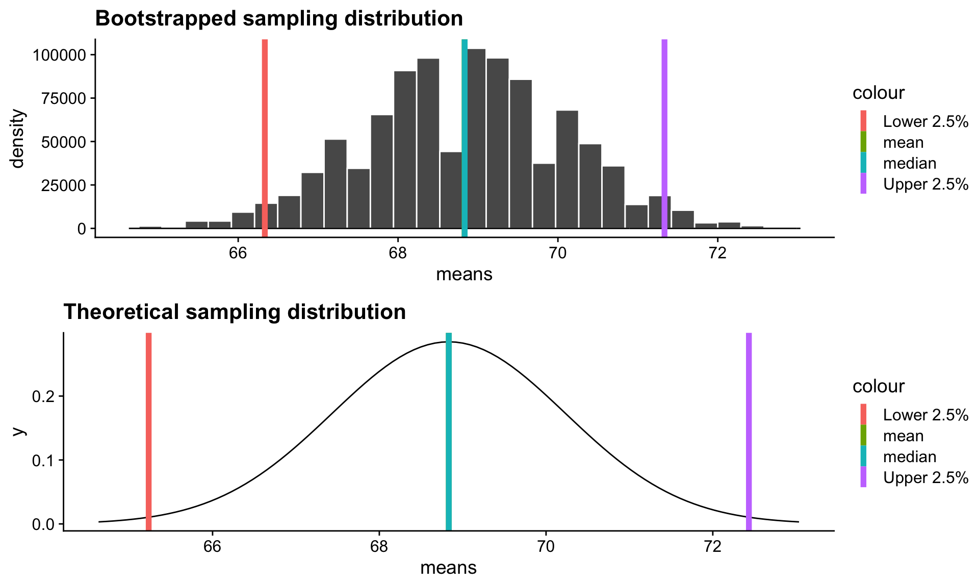
Hypothetical example:
A researcher examines the effect of caffeine on reaction times. Twenty-five participants had their reaction times measured before and after consuming caffeine. The units are in milliseconds, with baseline (pre-caffeine) reactions ranging roughly from 200-800ms.
Code to simulate data
# Set random seed
set.seed(112224)

# Generate skewed data using chi-square distributions
n <- 25
pre_caffeine <- rchisq(n, df=3) * 100 + 200
post_caffeine <- pre_caffeine - rchisq(n, df=2) * 20

# Create data frame
data <- data.frame(
  pre_caffeine = pre_caffeine,
  post_caffeine = post_caffeine,
  difference = pre_caffeine - post_caffeine
)
Assumptions of t-tests?
Independence
Normality
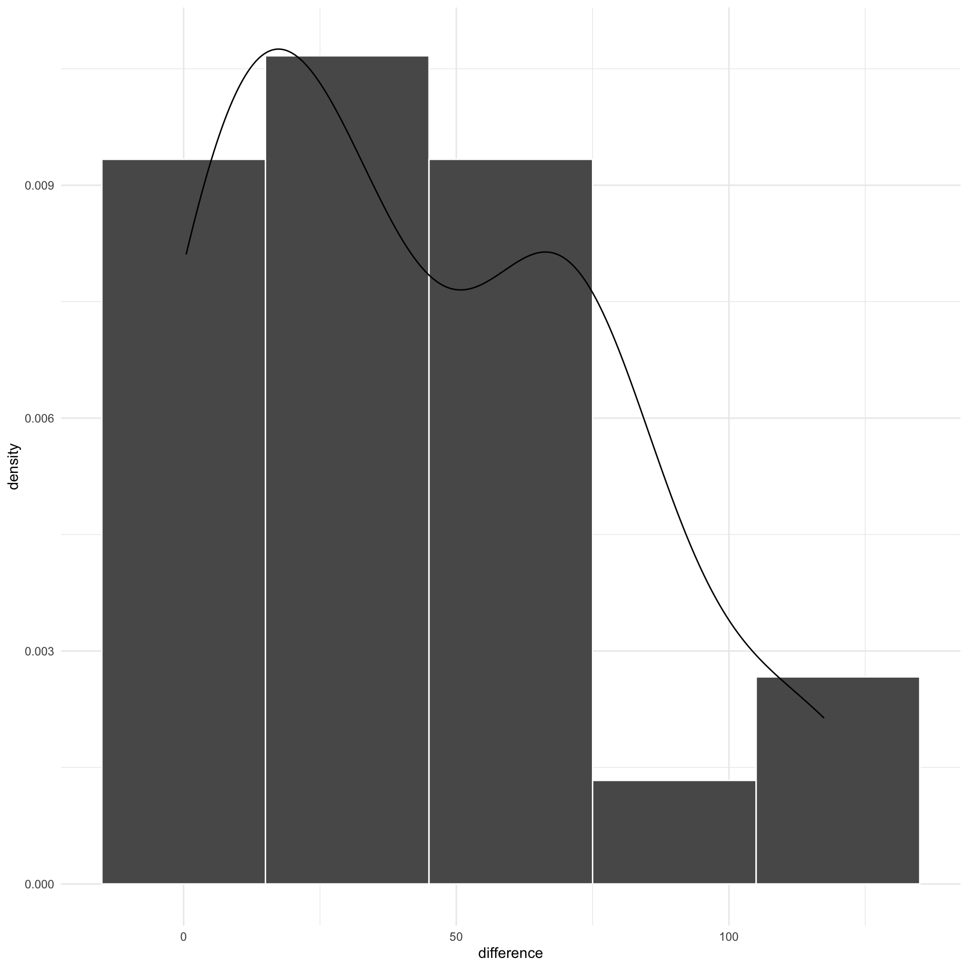
Not only are these data skewed, but we would expect the population distribution (reaction times) to be skewed as well.
Furthermore, our sample size (25) is small enough for us to give pause before applying the CLT.
We can’t reasonably meet the assumptions of a t-test, so we cannot use this test. Instead, we’ll use bootstrapping.
# how many simulations?
n_boots = 1000
# create an empty vector to hold results
boot_diff = numeric(length = 1000)
set.seed(112224) # set seed to ensure the random results are the same every time
for(i in 1:n_boots){
  # sample with replacement. new dataset is the same size as the original
  bootdata = data[sample(1:nrow(data), size = nrow(data), replace = T), ]
  # calculate mean in new dataset
  mean_diff = mean(bootdata$difference)
  # add to empty vector
  boot_diff[i] = mean_diff
}
head(boot_diff)
[1] 38.21266 42.10021 36.41429 45.51011 51.79053 38.15113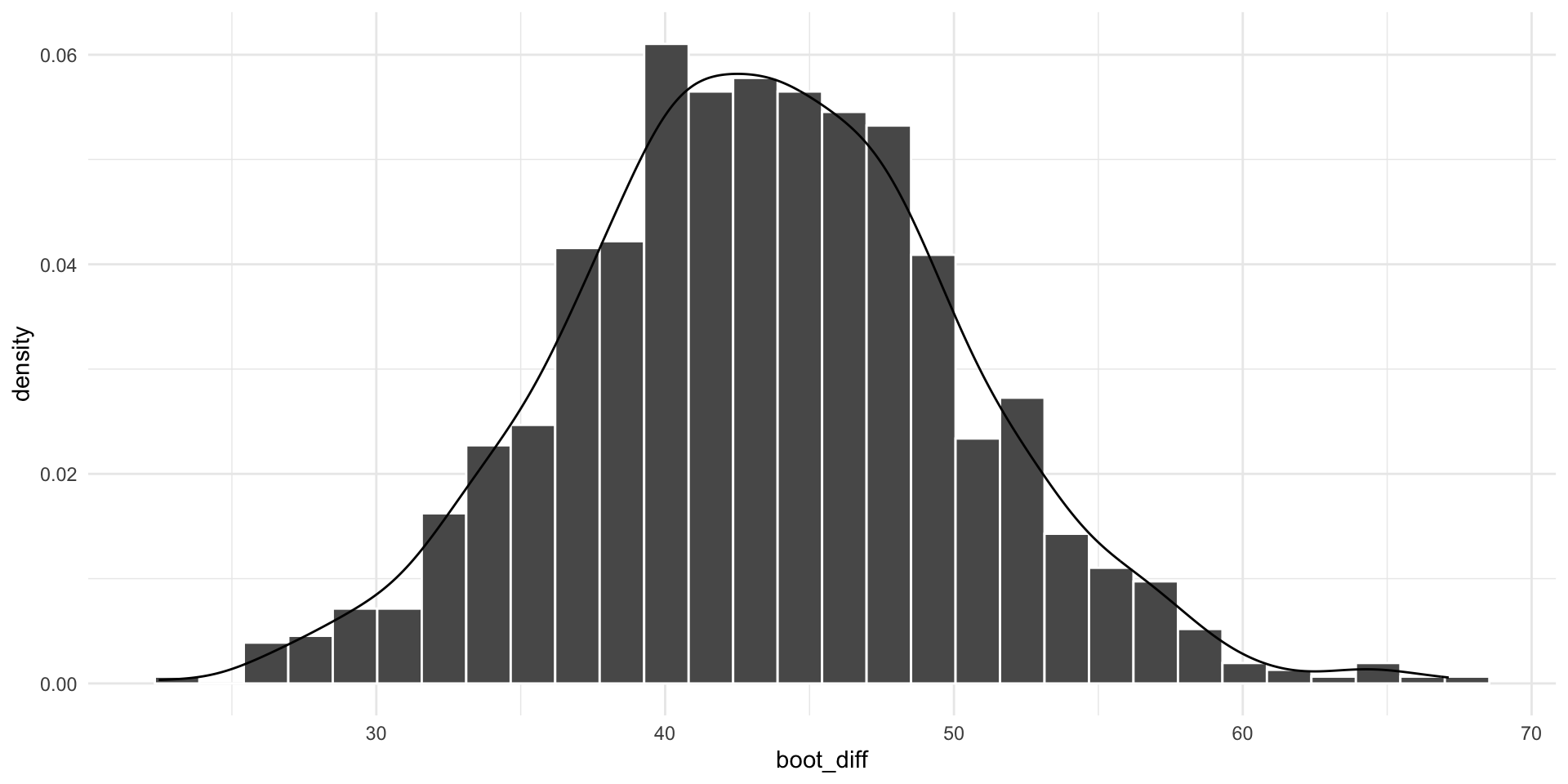
What’s the median bootstrapped difference?
What’s the empirical 95% CI?
Note: there is NO p-value for this test.
Bootstrapping can be used for any statistic you care about.

Are the variances of these groups different?
[1] 5242.314 4522.135 5491.403 8037.365 3989.397 8330.253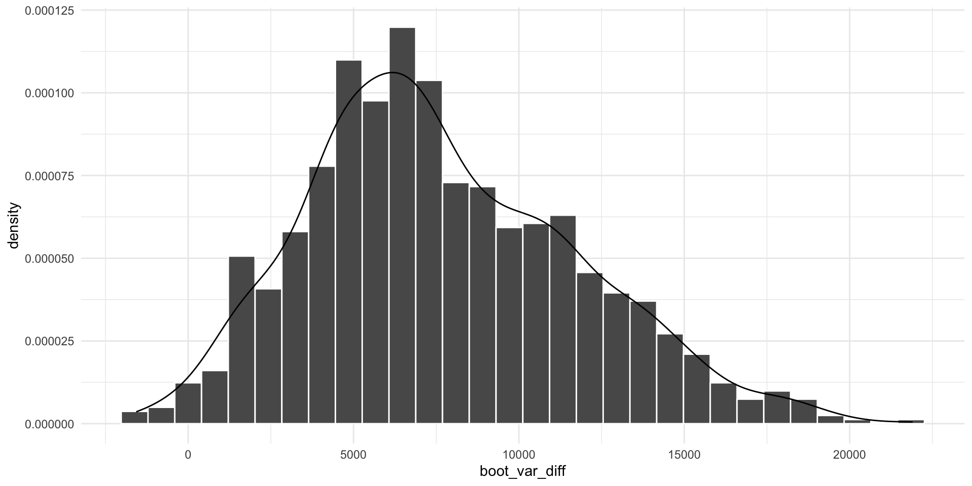
Wrap up and a look ahead
Most statistical methods propose some model, represented by linear combinations, and then tests how likely we would be to see data like ours under that model.
one-sample t-tests propose that a single value represents all the data
t-tests propose a model that two means differ
more complicated models propose that some combination of variables, categorical and continuous, govern the patterns in the data
As we think about where we’re going next term, it will be helpful to put some perspective on what we’ve covered already.
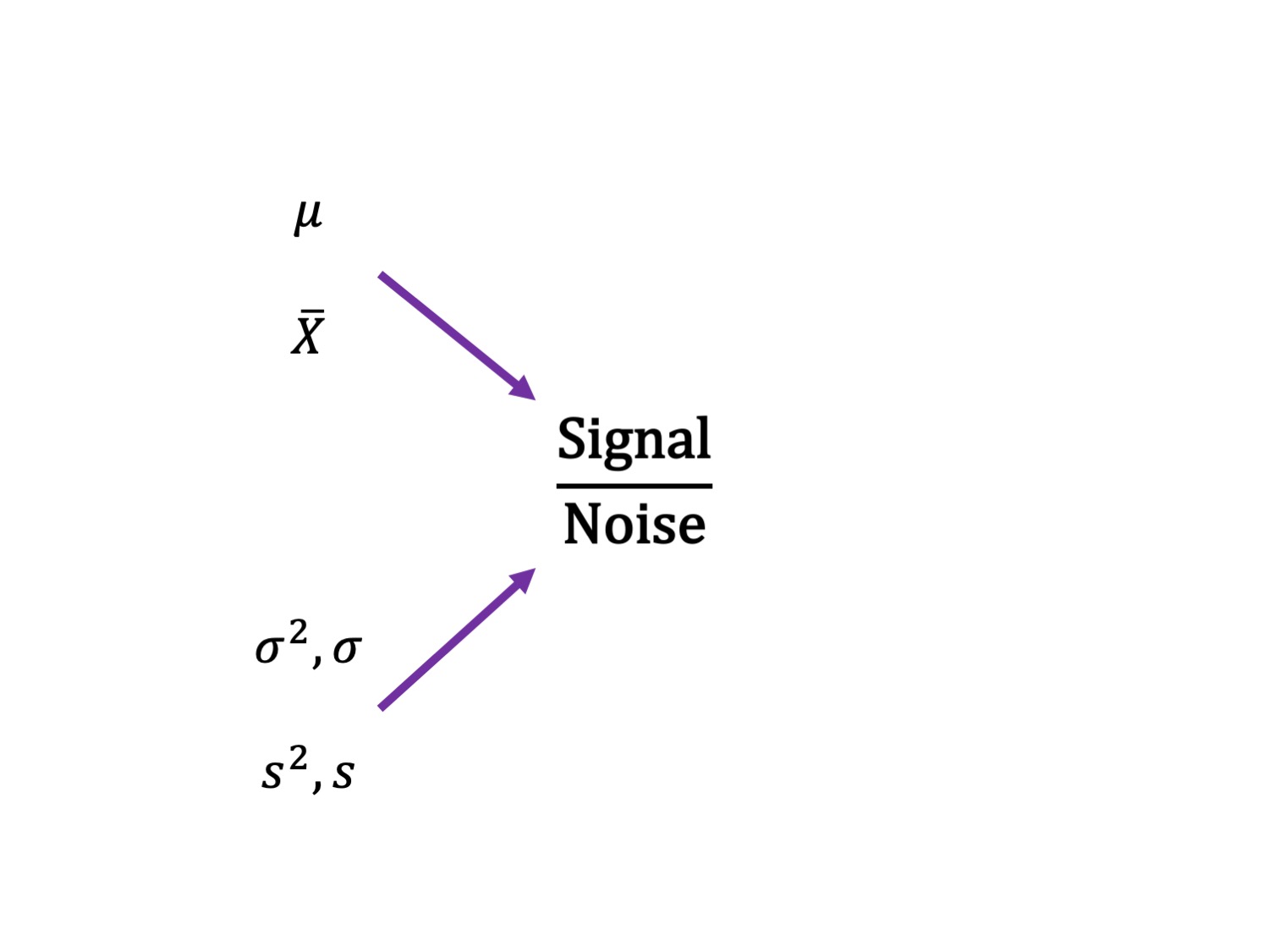
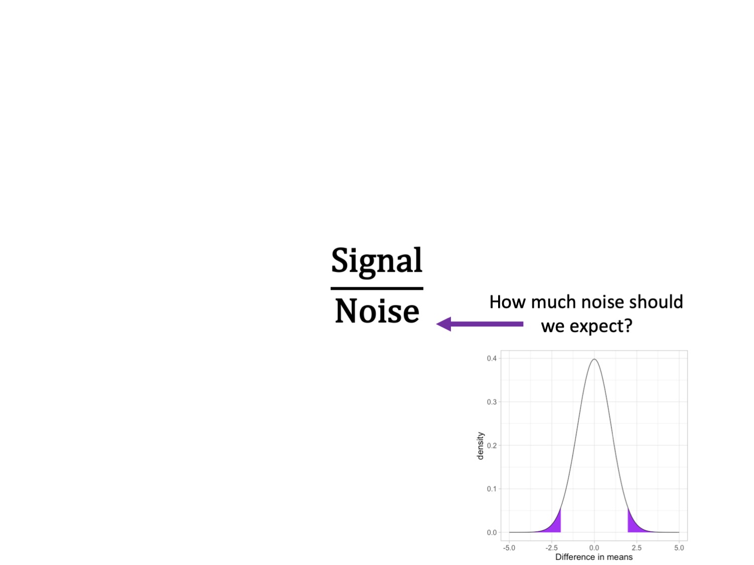
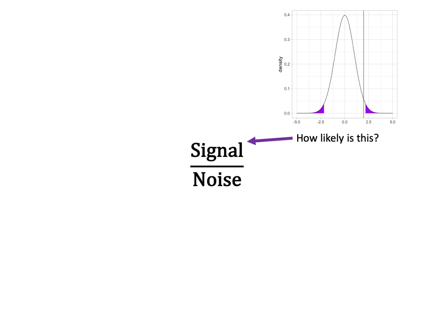
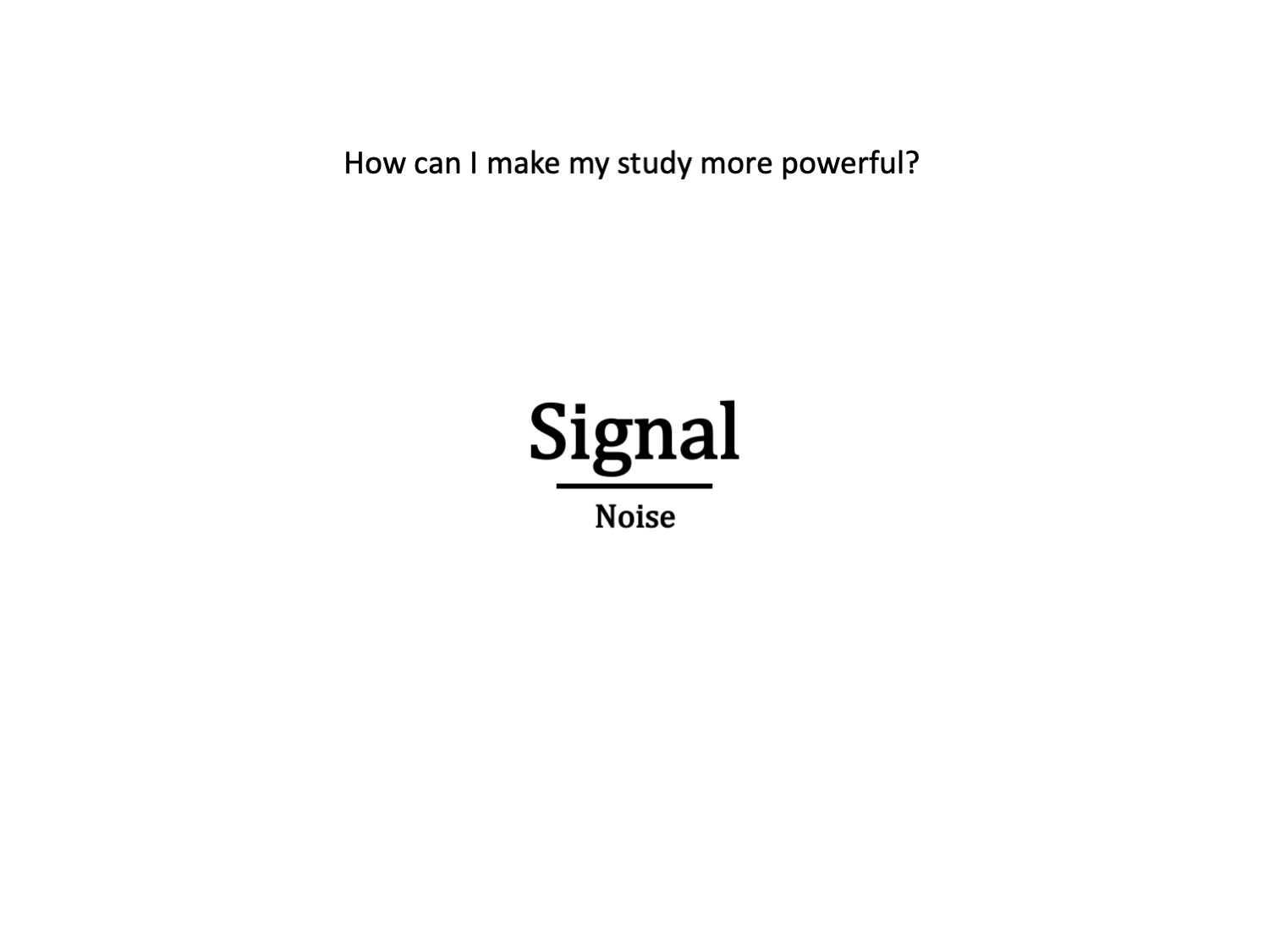
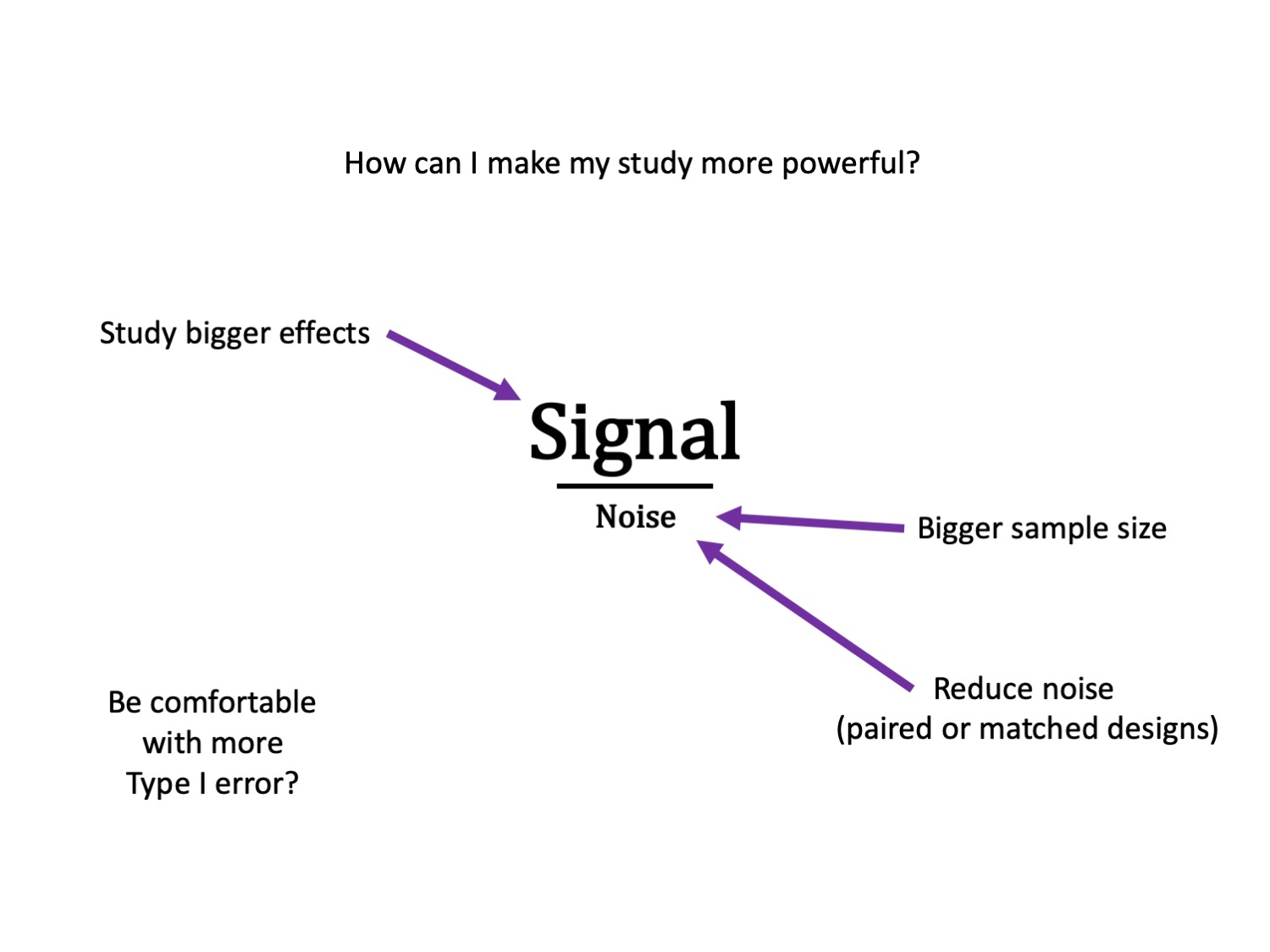
Because we’re using probability theory, we have to assume independence between trials.
- independent rolls of the die
- independent draws from a deck of cards
- independent… tests of hypotheses?
What happens when our tests are not independent of one another?
- What happens if I run multiple tests on one dataset?
The issue of independence between tests has long been ignored by scientists. It was only when we were confronted with impossible-to believe results (people have ESP) that we started to doubt our methods.
And an explosion of fraud cases made us revisit our incentive structures. Maybe we weren’t producing the best science we could…
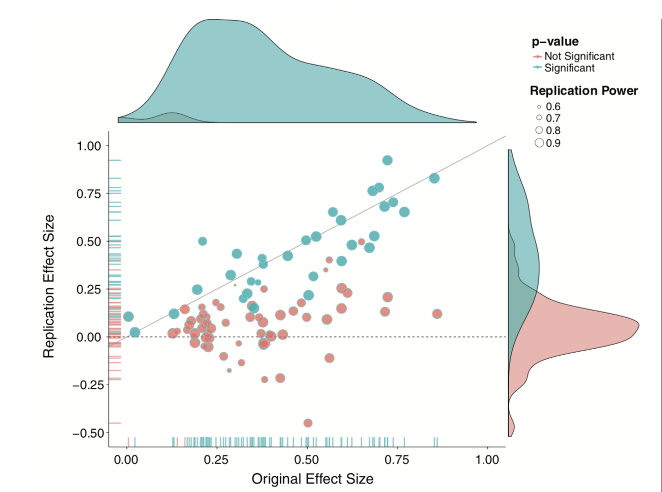
Since then (2011), there’s been greater push to revisit “known” effects in psychology and related fields, with sobering results.
The good news is that things seem to be changing, rapidly.
Independence isn’t the only assumption we have to make to conduct hypothesis tests.
We also make assumptions about the underlying populations.
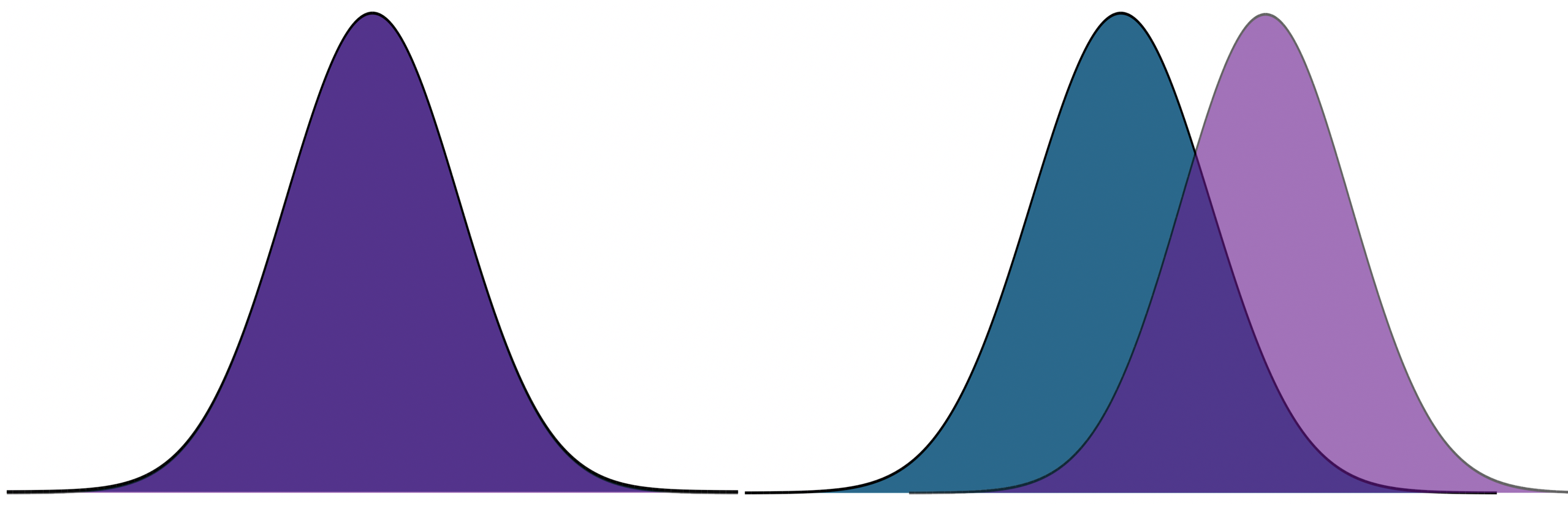
Normality
Homogeneity of variance
Sometimes we fail to meet those assumptions, in which case we may have to change course.
How big of a violation of the assumption is too much?
- It depends.
How do you know your operation X measures your construct A well?
- You don’t.
What should alpha be?
- You tell me.
Statistics is not a recipe book. It’s a tool box. And there are many ways to use your tools.
Your job is to
- Understand the tools well enough to know how and when to use them, and
- Be able to justify your methods.

Next time…
PSY 612 in 2025
(But first):
- Quiz 9 now
- Journal 10 due Monday night (PSY only)
- Oral exams next week
- Homework 3 due Monday (9am)
- All revisions due Friday (9am)