class: center, middle, inverse, title-slide # NHST II --- ## Review of key Points - The null hypothesis ( `\(H_0\)` ) is a claim about the particular value that a population parameter takes. - The alternative hypothesis ( `\(H_1\)` ) states an alternative range of values for the population parameter. - We test the null hypothesis by determining if we have sufficient evidence that contradicts or nullifies it. - We reject the null hypothesis if the data in hand are rare, unusual, or atypical if the null were true. The alternative hypothesis gains support when the null is rejected, but `\(H_1\)` is not proven. --- ### Review - If we do not reject `\(H_0\)`, that does not mean that we accept it. We have simply failed to reject it. It lives to fight another day. - A Z-statistic summarizes how unusual the sample estimate of a mean compared to the value of the mean as specified by the null hypothesis. - More broadly, we refer to the **test statistic** as the statistic that summarizes how unusual the sample estimate of a parameter is from the point value specified by the null hypothesis. --- ### Review - The test statistic is derived from a probability distribution that represents the likelihood of any sample estimated given that the null hypothesis is true. - We choose the probability assumption based on assumptions we are willing to make about the data. The **sampling distribution** of the test statistic tells us what counts as rare or unusual. --- ### Review - We summarize the probability of the sample data (or even more extreme data), assuming the null is true, by the ** `\(p\)`-value** (signified by `\(p\)`). This value is the proportion of the sampling distribution of the test statistic that is as extreme, or more extreme, as the test statistic value. If `\(p\)` is small, the observed data are unusual *if the null hypothesis is true*. If `\(p\)` is sufficiently small ( `\(p < .05\)` ), we may choose to reject the null hypothesis as a description of the data. --- ## `\(p\)`-values - Fisher established (rather arbitrarily) the sanctity of the .05 and .01 significance levels during his work in agriculture, including work on the effectiveness of fertilizer. A common source of fertilizer is cow manure. Male cattle are called bulls. A common misinterpretation of the p value ( `\(\alpha\)` ) is that it is the probability of the null hypothesis being wrong. Another common misunderstanding is that `\(1-\alpha\)` is the probability that results will replicate. --- - In most research, the probability that the null hypothesis is true is very small. If the null hypothesis is false, then the only mistake to be made is a failure to detect a real effect -- a Type II error. If- the null hypothesis is false, then the significance test is akin to a test of whether the sample size was large enough. - Because Null Hypothesis Significance Testing (NHST) is beginning to seem like a bit of a sham, some have suggested we start calling it Statistical Hypothesis Inference Testing. --- ## Errors In hypothesis testing, we can make two kinds of errors. | | Reject `\(H_0\)` | Do not reject | |------------:|:----------------:|:----------------:| | `\(H_0\)` True | Type I Error | Correct decision | | `\(H_0\)` False | Correct decision | Type II Error | Falsely rejecting the null hypothesis is a **Type I error**. Traditionally this has been viewed as particularly important to control at a low level (akin to avoiding false conviction of an innocent defendant). --- ## Errors In hypothesis testing, we can make two kinds of errors. | | Reject `\(H_0\)` | Do not reject | |------------:|:----------------:|:----------------:| | `\(H_0\)` True | Type I Error | Correct decision | | `\(H_0\)` False | Correct decision | Type II Error | Failing to reject the null hypothesis when it is false is a **Type II error**. This is sometimes viewed as a failure in signal detection. --- ## Errors In hypothesis testing, we can make two kinds of errors. | | Reject `\(H_0\)` | Do not reject | |------------:|:----------------:|:----------------:| | `\(H_0\)` True | Type I Error | Correct decision | | `\(H_0\)` False | Correct decision | Type II Error | Null hypothesis testing is designed to make it easy to control Type I errors. We set a minimum proportion of such errors that we would be willing to tolerate in the long run. This is the significance level ( `\(\alpha\)` ). By tradition this is no greater than .05. --- ## Errors In hypothesis testing, we can make two kinds of errors. | | Reject `\(H_0\)` | Do not reject | |------------:|:----------------:|:----------------:| | `\(H_0\)` True | Type I Error | Correct decision | | `\(H_0\)` False | Correct decision | Type II Error | Controlling Type II errors is more challenging because it depends on several factors. But, we usually DO want to control these errors. Some argue that the null hypothesis is usually false, so the only error we can make is a Type II error -- a failure to detect a signal that is present. **Power** is the probability of correctly rejecting a false null hypothesis. --- ### Some Greek letters `\(\alpha\)` -- The rate at which we make Type I errors, which is the same `\(\alpha\)` as the cut-off for `\(p\)` -values. `\(\beta\)` -- The rate at which we make Type II errors. `\(1-\beta\)` -- statistical power. Note that all these probability statements are being made in the frequentist sense -- in the long run, we expect to make Type I errors `\(\alpha\)` proportion of the time and Type II errors `\(\beta\)` proportion of the time. --- Controlling Type II errors is the goal of power analysis and must contend with four quantities that are interrelated: - Sample size - Effect size - Significance level ( `\(\alpha\)` ) - Power When any three are known, the remaining one can be determined. Usually this translates into determining the power present in a research design (**post-hoc power analysis** ), or, determining the sample size necessary to achieve a desired level of power. We must specify a specific value for the alternative hypothesis to estimate and control Type II errors. --- Suppose we have a measure of social sensitivity that we have administered to a random sample of 20 psychology students. This measure has a population mean ( `\(\mu\)` ) of 100 and a standard deviation ( `\(\sigma\)` ) of 20. We suspect that psychology students are more sensitive to others than is typical and want to know if their mean, which is 110, is sufficient evidence to reject the null hypothesis that they are no more sensitive than the rest of the population. We would also like to know how likely it is that we could make a mistake by concluding that psychology students are not different when they really are: A Type II error. --- .left-column[ .small[ We begin by defining the location in the null hypothesis distribution beyond which empirical results would be considered sufficiently unusual to lead us to reject the null hypothesis. We control these mistakes (Type I errors) at the chosen level of significance ( `\(\alpha = .05\)` ). ] ] <!-- --> ??? ### How do we figure out where this region is? Start with our `\(\alpha\)` level (.05) Given our distribution parameters, what Z-value corresponds to .05 above that line mu = 100 x = 110 s = 20 n = 20 sem = `\(\frac{20}{\sqrt{20}}\)` = 4.47 z = 1.64 --- .pull-left[ `$$\text{Critical Value} = \mu_0 + Z_{.95}\frac{\sigma}{\sqrt{N}}$$` ```r qnorm(.95) ``` ``` ## [1] 1.644854 ``` `$$\text{Critical Value} = 100 + 1.645\frac{20}{\sqrt{20}} = 107.4$$` What if the null hypothesis is false? How likely are we to correctly reject the null hypothesis in the long run? ] .pull-right[ <p>&nbsp;</p> <p>&nbsp;</p> <p>&nbsp;</p> <p>&nbsp;</p> <p>&nbsp;</p> <!-- --> ] --- .left-column[ .small[ To determine the probability of a Type II error we must specify a value for the alternative hypothesis. We will use the sample mean of 110. In the long run, if psychology samples have a mean of 110 ( `\(\sigma = 20\)`, `\(N = 20\)` ), we will correctly reject the null with probability of .72 (power). We will incorrectly fail to reject the null with probability of .28 ( `\(\beta\)` ). ] ] <!-- --> --- .pull-left[ <!-- --> Once the critical value and alternative value is established, we can determine the location of the critical value in the alternative distribution. ] -- .pull-right[ `$$Z_1 = \frac{CV_0 - \mu_1}{\frac{\sigma}{\sqrt{N}}}$$` `$$Z_1 = \frac{107.4 - 110}{\frac{20}{\sqrt{20}}} = -.59$$` The proportion of the alternative distribution that falls below that point is the probability of a Type II error (.28); power is then .72. ```r pnorm(-.59) ``` ``` ## [1] 0.2775953 ``` ] --- The choice of 110 as the mean of `\(H_1\)` is completely arbirtary. What if we believe that the alternative mean is 115? This larger signal should be easier to detect. .pull-left[ 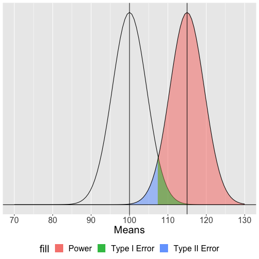<!-- --> ] .pull-right[ `$$Z_1 = \frac{107.4 - 115}{\frac{20}{\sqrt{20}}} = -1.71$$` ```r 1-pnorm(-1.71) ``` ``` ## [1] 0.9563671 ``` ] --- What if instead we increase the sample size? This will reduce variability in the sampling distribution, making the difference between the null and alternative distributions easier to see. .pull-left[ 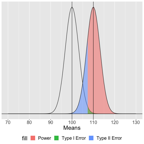<!-- --> ] .pull-right[ `$$\text{Critical Value} = 100 + 1.645\frac{20}{\sqrt{40}} = 105.2$$` `$$Z_1 = \frac{105.2 - 110}{\frac{20}{\sqrt{40}}} = -1.52$$` ```r 1-pnorm(-1.52) ``` ``` ## [1] 0.9357445 ``` ] --- What if we decrease the significance level to .025? <p>&nbsp;</p> .pull-left[ <!-- --> ] .pull-right[ That will move the critical value: `$$CV_0 = 100 + 1.96[\frac{20}{\sqrt{20}}] = 108.8$$` `$$Z_1 = \frac{108.8 - 110}{\frac{20}{\sqrt{20}}} = -.28$$` ```r 1-pnorm(-.28) ``` ``` ## [1] 0.6102612 ``` ] I strongly recommend playing around with different configurations of `\(N\)`, `\(\alpha\)` and the difference in means ( `\(d\)` ) in this [online demo](https://rpsychologist.com/d3/NHST/). --- More generally we can determine the relationship between effect size and power for a constant `\(\alpha\)` (.05) and sample size ( `\(N = 20\)` ). 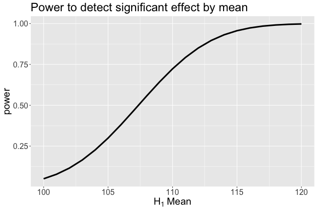<!-- --> --- Likewise, we can display the relationship between sample size and power for a constant `\(\alpha\)` and effect size. 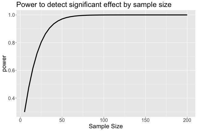<!-- --> --- Power changes as a function of significance level for a constant effect size and sample size. 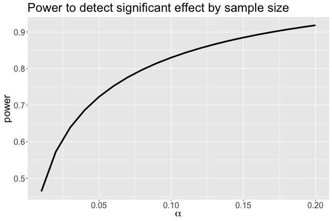<!-- --> --- For a two-tailed test, we divide the rejection area equally in the two tails. If `\(\alpha = .05\)`, then each tail contains .025 and critical values will be 1.96 standard errors away from the null mean. 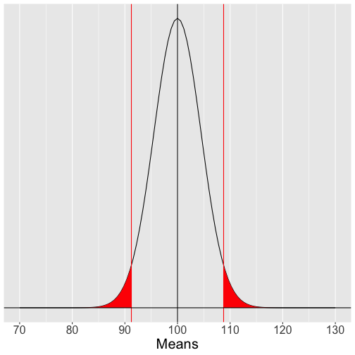<!-- --> --- The relationship of power to effect size is more complicated because deviations above and below the null mean are relevant. 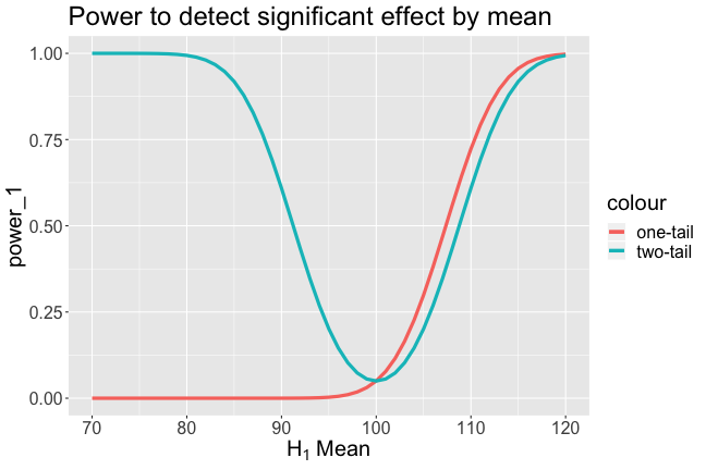<!-- --> --- A two-tailed test is less powerful (more conservative) than a one-tailed test for the same sample size. 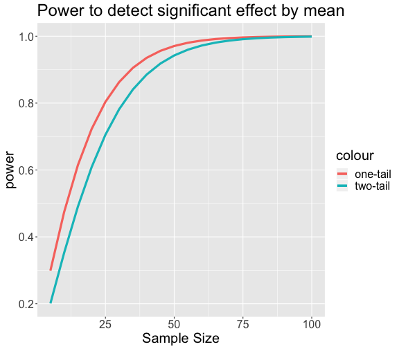<!-- --> --- <!-- --> --- ### How can power be increased? .pull-left[ <!-- --> ] .pull-right[ `$$Z_1 = \frac{CV_0 - \mu_1}{\frac{\sigma}{\sqrt{N}}}$$` - increase `\(\mu_1\)` - decrease `\(CV_0\)` - increase `\(N\)` - reduce `\(\sigma\)` ] --- Often the most challenging part of a power analysis is to settle on an effect size. - Past research can often provide some guidance, especially if a meta-analysis is available. - Note that these are often over-estimates. - Sometimes a field might have standards regarding what counts as a meaningful effect (e.g., minimal clinically important difference). - Lacking this information, we can settle for more abstract benchmarks or rules of thumb about what are “small,” “medium”, and “large” effects. - But as we discussed, these benchmarks need to be contextualized in real-world outcomes. - Complicating these choices, effect sizes come in a variety of metrics. --- ### Prevalence of false positives Consider where `\(\alpha\)`, `\(\beta\)` and power fall in this grid. | | Reject `\(H_0\)` | Do not reject | |------------:|:----------------:|:----------------:| | `\(H_0\)` True | Type I Error | Correct decision | | `\(H_0\)` False | Correct decision | Type II Error | --- ### Prevalence of false positives Consider where `\(\alpha\)`, `\(\beta\)` and power fall in this grid. | | Reject `\(H_0\)` | Do not reject | |------------:|:----------------:|:----------------:| | `\(H_0\)` True | `\(\alpha\)` | `\(1-\beta\)` | | `\(H_0\)` False | `\(1-\alpha\)` | `\(\beta\)` | What is the sum of these cells? --- ### Prevalence of false positives Figuring out how common Type I and Type II errors are in a literature requires an additional piece of information: - How often `\(H_0\)` is true. [Ioannidis (2005)](../readings/Ioannidis_2005.pdf) demonstrates that given R (the ratio of `\(H_0\)` false over `\(H-0\)` true), we can calculate the **positive predictive value** of a finding, which is the likelihood that `\(H_1\)` is true given we found a significant result: `$$\frac{(1-\beta)R}{(1-\beta)R+\alpha}$$` ??? Note that given publication bias, or the tendancy to only publish significant results, PPV can be thought of as the likelihood of a given published study being a false positive. --- Let's make some assumptions. If psychology studies use `\(\alpha = .05\)` and are good at achieving adequate power ( `\(1-\beta = .80\)` ), how does the choice of hypothesis affect PPV? <!-- --> --- However, there are many reasons to think that psychology studies are underpowered. Typical power may be closer to .5 or even worse. <!-- --> --- In addition to being under-powered, there's recognition that research practices have inflated family-wise error, making `\(\alpha\)` much bigger than it should be. 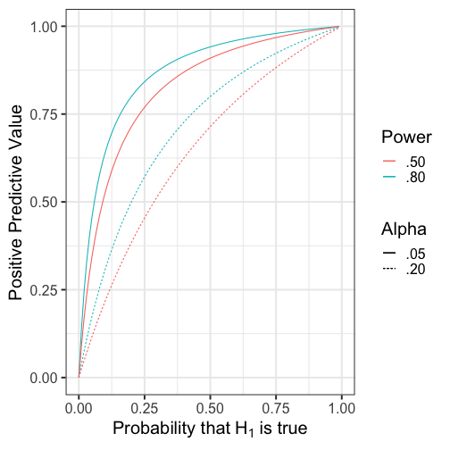<!-- --> --- 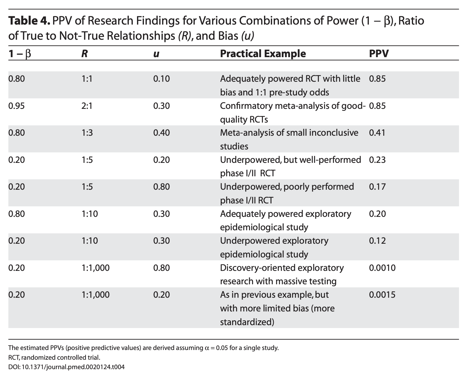 --- class: inverse ## Next time... critiques of NHST