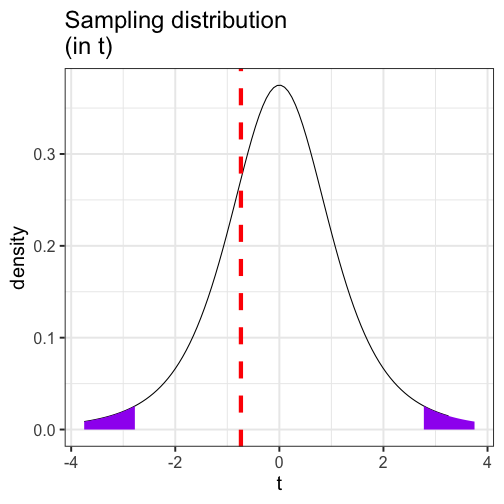
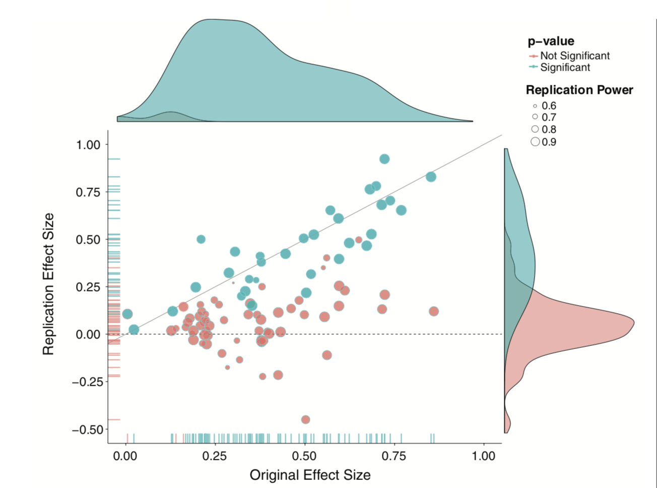
Comparing two means and fall term wrap-up

# Comparing two means and fall term wrap-up

---

### Office hours during finals week

Cam: Monday, 12pm-2pm

Brenden: Available by appointment Tuesday

Sara: Available by appointment Mon-Thurs

### Advice

Your textbook is a good resource.

---

## Example

You have good reason to believe that dogs are smarter than cats. You design a study in which you recruit dogs and cats from households that have one of each and conduct a series of IQ tests to measure each animal's intelligence on a scale from 1 (not so smart) to 5 (genius).

| Cat | Dog |
|:---:|:---:|
|2 | 1|
|5 | 4|
|3 | 3|
|1 | 3|
|2 | 5|

---

```r
pets = data.frame(cat = c(2,5,3,1,2), 
                  dog = c(1,4,3,3,5))

pets$difference = pets$cat-pets$dog

psych::describe(pets, fast = T)
```

```
##            vars n mean   sd min max range   se
## cat           1 5  2.6 1.52   1   5     4 0.68
## dog           2 5  3.2 1.48   1   5     4 0.66
## difference    3 5 -0.6 1.82  -3   1     4 0.81
```

`$$\large \frac{\hat{\sigma}_\Delta}{\sqrt{N}} = \frac{1.82}{\sqrt{5}} = 0.81$$`

`$$\large t = \frac{\bar{\Delta}}{\frac{\hat{\sigma}_\Delta}{\sqrt{N}}} = \frac{-0.60}{0.81} = -0.74$$`
---

![](18-two_means_IV_files/figure-html/unnamed-chunk-2-1.png)

---

We can also calculate the area at least as far away from the null as our test statistic.

```r
stat = mean(pets$difference)/(sd(pets$difference)/sqrt(5))
pt(abs(stat), df = 5-1, lower.tail = F)
```

```
## [1] 0.2505847
```

```r
pt(abs(stat), df = 5-1, lower.tail = F)*2
```

```
## [1] 0.5011694
```

---

## *t*-tests and Matrix Algebra

### Independent-samples *t*-test

At it's heart, the independent samples *t*-test proposes a model in which our best guess of a person's score is the mean of their group.

We can use **linear combinations** of both rows and columns to generate these "best guess" scores.

---
Assume your data take the following form:

`$$\large \mathbf{X} = \left(\begin{array}
{rr}
\text{Party} & \text{Age} \\
D & 85.9  \\
R & 78.8  \\
\vdots & \vdots  \\
D & 83.2 
\end{array}\right)$$`
]

What are your linear combinations of rows?
]

**Linear combinations of columns:**

`$$\large \mathbf{T_C} = \left(\begin{array}
{r}
0 \\
1
\end{array}\right)$$`

---
Assume your data take the following form:

`$$\large \mathbf{X} = \left(\begin{array}
{rr}
\text{Party} & \text{Age} \\
D & 85.9  \\
R & 78.8  \\
\vdots & \vdots  \\
D & 83.2 
\end{array}\right)$$`
]

What are your linear combinations of rows?
]

**Linear combinations of rows:**

`$$\mathbf{T_R} = \left(\begin{array}
{rrrr}
\frac{1}{N_D} & 0 & \dots & \frac{1}{N_D} \\
0 & \frac{1}{N_R} & \dots & 0 \\
\end{array}\right)$$`

---

`$$(T_R)X(T_C) = M$$`

This set of linear combinations calculates the different means of our two groups. That's great!

But there's another way. We can create a single transformation matrix, \large \mathbf{T}, that's very simple:

`$$\mathbf{T} = \left(\begin{array}
{rr}
1 & 0 \\
1 & 1 \\
\vdots & \vdots  \\
1 & 0 \\
\end{array}\right)$$`

Using this matrix, we can solve a different equation:

`$$(T'T)^{-1}T'X = (b)$$`
In this case, *b* will be a vector with 2 scalars.

---

```r
X = congress$age
T_mat = matrix(1, ncol = 2, nrow = length(X))
T_mat[congress$party == "D", 2] = 0
```

```
##      [,1] [,2]
## [1,]    1    1
## [2,]    1    0
## [3,]    1    0
## [4,]    1    0
## [5,]    1    0
## [6,]    1    1
```

`$$(T'T)^{-1}T'X = (b)$$`

```r
solve(t(T_mat) %*% T_mat) %*% t(T_mat) %*% X
```

```
##           [,1]
## [1,] 59.550965
## [2,] -3.768633
```

What do these numbers represent?

???

`$$\Large \bar{X} = T\mathbf{X} = 1'\mathbf{X}(1'1)^{-1}$$`

---

### Standard errors

We can use the same matrix, `$\large \mathbf{T}$` , to transform the variance-covariance into standard errors.

`$$\large  \text{Var}_b = \hat{\sigma}^2(T'T)^{-1}$$`

We use the pooled variance, instead of the empirical estimate.

```r
var1 = var(congress$age[congress$party == "D"])
var2 = var(congress$age[congress$party == "R"])
n1 = length(which(congress$party == "D"))
n2 = length(which(congress$party == "R"))
pooled = ((n1-1)*var1 +(n2-1)*var2)/(n1+n2-2)
```

```r
pooled * solve(t(T_mat) %*% T_mat)
```

```
##            [,1]       [,2]
## [1,]  0.4473336 -0.4473336
## [2,] -0.4473336  0.8567308
```

---

```r
solve(t(T_mat) %*% T_mat) %*% t(T_mat) %*% X
```

```
##           [,1]
## [1,] 59.550965
## [2,] -3.768633
```
]

```r
pooled * solve(t(T_mat) %*% T_mat)
```

```
##            [,1]       [,2]
## [1,]  0.4473336 -0.4473336
## [2,] -0.4473336  0.8567308
```
]

This is a one-sample *t*-test comparing the mean of the reference group to 0.

]

This is an independent-samples *t*-test comparing the mean of the two groups.
]

---

## *t*-tests and Matrix Algebra

### Paired-samples *t*-test

The algebra for the paired-samples *t*-test is actually quite simple, because the difference score is a very simple weighted linear combination:

`$$LC_i = W_1X_{1,i} + W_2X_{2,i} + \dots + W_kX_{k,i}$$`

The variance of a weighted linear combination is a function of the weights (W) applied the variance-covariance matrix:

`$$\large \left[\begin{array}
{rr} 
W_1 & W_2
\end{array}\right]
\left[\begin{array}
{rr} 
\hat{\sigma}^2_{X_1} & \hat{\sigma}_{X_1X_2} \\
\hat{\sigma}_{X_2X_1} & \hat{\sigma}^2_{X_1}
\end{array}\right]
\left[\begin{array}
{r} 
W_1 \\
W_2
\end{array} 
\right]$$`

]

???
What is the linear combination?

Difference = At - Away

Difference = (1)At + (-1)Away

---

```r
X = as.matrix(gulls[, c("At", "Away")])
W = c(1, -1)
```

```r
X %*% W
```

```
##       [,1]
##  [1,]  175
##  [2,]  220
##  [3,]    3
##  [4,]   -3
##  [5,]   34
##  [6,]   21
##  [7,]   -9
##  [8,]    1
##  [9,]  282
## [10,]  294
## [11,]    3
## [12,]    1
## [13,]   -2
## [14,]   -7
## [15,]  294
## [16,]   47
## [17,]  134
## [18,]  -42
## [19,]  133
```
]

```r
(V_X = cov(X))
```

```
##             At     Away
## At   18269.760 3719.675
## Away  3719.675 2590.468
```

```r
(V_Difference = W %*% V_X %*% W)
```

```
##          [,1]
## [1,] 13420.88
```

```r
sqrt(V_Difference)
```

```
##          [,1]
## [1,] 115.8485
```

]

---

### Matrix Algebra

There is nothing particularly special about difference scores `$(W = 1, -1)$`. Any conceptually sensible weights can be used to create  linear combinations, which can then be used in hypothesis tests:

`$$t = \frac{\bar{LC}-\mu}{\frac{\hat{\sigma}_{LC}}{\sqrt{N}}}$$`

In other words: you can test **any linear combination** of variables against **any null hypothesis** using this formula. You are not limited to differences in means or nil hypotheses `$\large (\mu=0)$`.

---

Building and testing linear combinations of variables is nearly everything we'll do in PSY 612.

Most statistical methods propose some model, represented by linear combinations, and then tests how likely we would be to seee data like ours under that model.

* one-sample *t*-tests propose that a single value represents all the data

* *t*-tests propose a model that two means differ

* more complicated models propose that some comination of variables, categorical and continuous, govern the patterns in the data

---

We'll spend most of PSY 612 talking about different ways of building and testing models, but at their heart, all will use a combination of

`$$(T'T)^{-1}T'X = (b)$$`

`$$LC_i = W_1X_{1,i} + W_2X_{2,i} + \dots + W_kX_{k,i}$$`

As we think about where we're going next term, it will be helpful to put some perspective on what we've covered already.

---

---

---

---

---

---

---

Because we're using probability theory, we have to assume independence between trials.

* independent rolls of the die
* independent draws from a deck of cards
* independent... tests of hypotheses?

What happens when our tests are not independent of one another?

* For example, what happens if I only add a covariate to a model if the original covariate-less model is not significant?

* Similarly, what happens if I run multiple tests on one dataset?

---

The issue of independence between tests has long been ignored by scientists. It was only when we were confronted with impossible-to believe results (people have ESP, listening to "When I'm Sixty-Four" by The Beatles makes you younger) that we started to doubt our methods.

And an explosion of fraud cases made us revisit our incentive structures. Maybe we weren't producing the best science we could...

Since then (2011), there's been greater push to revisit "known" effects in psychology and related fields, with sobering results.

The good news is that things seem to be changing, rapidly.
]

---

Independence isn't the only assumption we have to make to conduct hypothesis tests.

We also make assumptions about the underlying populations.

![](images/null.png)
.pull-left[Normality]
.pull-right[Homogeneity of variance]

&nbsp;&nbsp;
Sometimes we fail to meet those assumptions, in which case we may have to change course.

---

How big of a violation of the assumption is too much?

* It depends.

How do you know your operation X measures your construct A well?

* You don't.

What should alpha be?

* You tell me.

---

.pull-left[
Statistics is not a recipe book. It's a tool box. And there are many ways to use your tools.

Your job is to 
1. Understand the tools well enough to know how and when to use them, and
2. Be able to justify your methods.

]

---

## Next time...

PSY 612 in 2020