class: center, middle, inverse, title-slide # Describing Data II --- class: inverse ### Annoucements - That quiz, huh? - Strategic breakout groups in lab - Homework 1 due in two weeks --- ### Last time .pull-left[### Population Variability **Sums of squares** `$$\small SS = \Sigma(X_i-\mu_x)^2$$` **Variance** `$$\small \sigma^2 = \frac{\Sigma(X_i-\mu_x)^2}{N} = \frac{SS}{N}$$` **Standard devation** `$$\scriptsize \sigma = \sqrt{\frac{\Sigma(X_i-\mu_x)^2}{N}}= \sqrt{\frac{SS}{N}} = \sqrt{\sigma^2}$$`] .pull-right[ ###Sample variability **Sums of squares** `$$\small SS = \Sigma(X_i-\bar{X})^2$$` **Variance** `$$\small s^2 = \frac{\Sigma(X_i-\bar{X})^2}{N-1} = \frac{SS}{N-1}$$` **Standard devation** `$$\scriptsize s = \sqrt{\frac{\Sigma(X_i-\bar{X})^2}{N-1}}= \sqrt{\frac{SS}{N-1}} = \sqrt{s^2}$$`] --- ## Bi-variate descriptives ### Covariation "Sum of the cross-products" ### Population `$$SP_{XY} =\Sigma(X_i−\mu_X)(Y_i−\mu_Y)$$` ### Sample $$ SP_{XY} =\Sigma(X_i−\bar{X})(Y_i−\bar{Y})$$ ??? **What does a large, positive SP indicate?** A positive relationship, same sign **What does a large, negatve SP indicate?** A negative relationship, different sign **What does SP close to 0 indicate?** No relationship --- ## Covariance Sort of like the variance of two variables ### Population `$$\sigma_{XY} =\frac{\Sigma(X_i−\mu_X)(Y_i−\mu_Y)}{N}$$` ### Sample `$$s_{XY} = cov_{XY} =\frac{\Sigma(X_i−\bar{X})(Y_i−\bar{Y})}{N-1}$$` --- ## Covariance table .large[ `$$\Large \mathbf{K_{XX}} = \left[\begin{array} {rrr} \sigma^2_X & cov_{XY} & cov_{XZ} \\ cov_{YX} & \sigma^2_Y & cov_{YZ} \\ cov_{ZX} & cov_{ZY} & \sigma^2_Z \end{array}\right]$$` ] ??? Point out that `\(cov_{xy}\)` is the same as `\(cov_{yx}\)` **Write on board:** `\(cov_{xy} = 126.5\)` `\(cov_{xz} = 5.2\)` Which variable, Y or Z, does X have greater relationship with? Can't know because you don't know what units they're measured in! --- ## Correlation - Measure of association - How much two variables are *linearly* related - -1 to 1 - Sign indicates direction of relationship - Invariant to changes in mean or scaling --- ## Correlation Pearson product moment correlation ### Population `$$\rho_{XY} = \frac{\Sigma z_Xz_Y}{N} = \frac{SP}{\sqrt{SS_X}\sqrt{SS_Y}} = \frac{\sigma_{XY}}{\sigma_X \sigma_Y}$$` ### Sample `$$r_{XY} = \frac{\Sigma z_Xz_Y}{n-1} = \frac{SP}{\sqrt{SS_X}\sqrt{SS_Y}} = \frac{s_{XY}}{s_X s_Y}$$` ??? **Why is it called the Pearson Product Moment correlation?** Pearson = Karl Pearson Product = multiply Moment = variance is the second moment of a distribution --- ```r data %>% ggplot(aes(x = x, y = y)) + geom_point(size = 3) + theme_bw() ``` 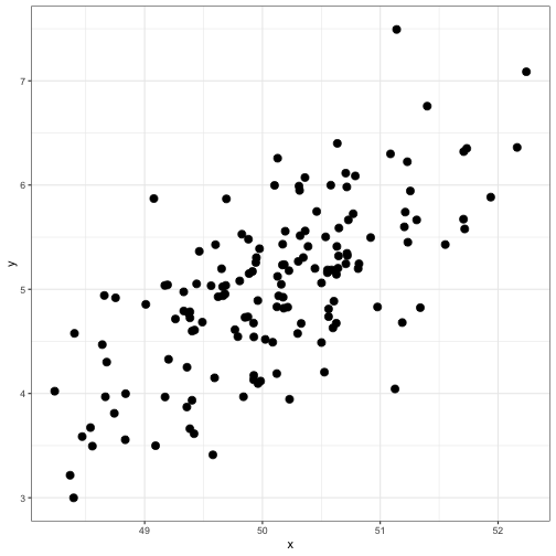<!-- --> What is the correlation between these two variables? ??? Correlation = 0.68 --- ```r data %>% ggplot(aes(x = x, y = y)) + geom_point(size = 3) + theme_bw() ``` 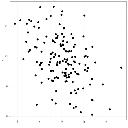<!-- --> What is the correlation between these two variables? ??? Correlation = -0.41 --- ```r data %>% ggplot(aes(x = x, y = y)) + geom_point(size = 3) + theme_bw() ``` 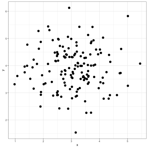<!-- --> What is the correlation between these two variables? ??? Correlation = 0 --- ## Effect size - Recall that *z*-scores allow us to compare across units of measure; the products of standardized scores are themselves standardized. - The correlation coefficient is a **standardized effect size** which can be used communicate the strength of a relationship. - Correlations can be compared across studies, measures, constructs, time. - Example: the correlation between age and height among children is `\(r = .70\)`. The correlation between self- and other-ratings of extraversion is `\(r = .25\)`. --- ## What is a large correlation? -- - [Cohen (1988)](http://www.utstat.toronto.edu/~brunner/oldclass/378f16/readings/CohenPower.pdf): .1 (small), .3 (medium), .5 (large) - Often forgot: Cohen said only to use them when you had nothing else to go on, and has since regretted even suggesting benchmarks to begin with. -- - [Rosenthal & Rubin (1982)](https://psycnet.apa.org/fulltext/1982-22591-001.pdf): life and death (the Binomial Effect Size Display) - treatment success rate `\(= .50 + .5(r)\)` and the control success rate `\(= .50 - .5(r)\)`. -- - `\(r^2\)`: Proportion of variance "explained" - [Ozer & Funder (2019)](https://uopsych.github.io/psy611/readings/Ozer_Funder_2019.pdf) claim this is misleading and nonsensical - Fisher (2019) suggests this particular argument is non-scientific (follow up [here](https://twitter.com/aaronjfisher/status/1168252269797629952) and then [here](https://www.psychologytoday.com/us/blog/personal-and-precise/201909/can-we-get-it-right-without-needing-be-right)) --- ### In breakout groups Order the following effect sizes from smallest to largest: - people attribute failures to bad luck - High elevations have lower annual temps - Ibuprofen and pain relief - scarcity increases the perceived value of a commodity - people in a bad mood are more aggressive - communicators perceived as more credible are more persuasive - Men weigh more than women - SES and IQ predicting mortality - Antihistomine and symptom relief - Height and weight among adults What would you guess each effect size is? ??? **What are good benchmarks?** - people attribute failures to bad luck ($r = .10$), - communicators perceived as more credible are more persuasive ($r = .10$) - Antihistomine and symptom relief: `\(r = .11\)` - scarcity increases the perceived value of a commodity ($r = .12$), - Ibuprofen and pain relief: `\(r = .14\)` - SES and IQ predicting mortality `\(r = 25\)` - Men weigh more than women: `\(r = .26\)` - High elevations have lower annual temps: `\(r = .34\)` - Classic social psych studies: `\(r\)` between .35 and .45 - people in a bad mood are more aggressive ($r = .41$) - Height and weight among `\(r = .44\)` **Implications** - Don't dismiss small effects - Be skeptical of large effects --- # Funder & Ozer (2019) - Effect sizes are often mis-interpreted. How? - What can fix this? - Pitfalls of small effects and large effects - Recommendations? ??? "benchmarks" lack context and are arbitrary `\(r^2\)` is stupid and worded in a way that makes it sound more causal than it is fix: - better benchmarks - compare with classic studies or other literature or all literature - compare with non-psychological phenomenon - explain in terms of consequences - BESD - long-run consequences **Recommendations** - Report effect sizes - Use large samples -- remember bias? - Report effect sizes in context - Stop using empty terminology - Revise guildelines --- ## What affects correlations? It's not enough to calculate a correlation between two variables. You should always look at a figure of the data to make sure the number accurately describes the relationship. Correlations can be easily fooled by qualities of your data, like: - Skewed distributions - Outliers - Restriction of range - Nonlinearity --- ## Skewed distributions ```r p = data %>% ggplot(aes(x=x, y=y)) + geom_point() ggMarginal(p, type = "density") ``` 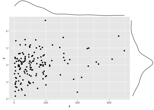<!-- --> --- ## Outliers ```r data %>% ggplot(aes(x=x, y=y)) + geom_point() ``` <!-- --> --- ## Outliers ```r data %>% ggplot(aes(x=x, y=y)) + geom_point() + geom_smooth(method = "lm", se = FALSE, color = "red") + geom_smooth(data = data[-51,], method = "lm", se = FALSE) ``` ``` ## `geom_smooth()` using formula 'y ~ x' ## `geom_smooth()` using formula 'y ~ x' ``` <!-- --> --- ## Outliers ```r data %>% ggplot(aes(x=x, y=y)) + geom_point() + geom_smooth(method = "lm", se = FALSE, color = "red") + geom_smooth(data = data[-c(n+1),], method = "lm", se = FALSE) ``` ``` ## `geom_smooth()` using formula 'y ~ x' ## `geom_smooth()` using formula 'y ~ x' ``` <!-- --> --- ## Restriction of range ```r data %>% ggplot(aes(x=x, y=y)) + geom_point() + geom_smooth(method = "lm", se = FALSE, color = "red") ``` ``` ## `geom_smooth()` using formula 'y ~ x' ``` <!-- --> ??? What if I told you there were scores on X could range from 97 to 103? --- ## Restriction of range ```r data %>% ggplot(aes(x=x, y=y)) + geom_point() + geom_smooth(method = "lm", se = FALSE, color = "red") + geom_point(data = real_data) + geom_smooth(method = "lm", se = FALSE, data = real_data, color = "blue") ``` ``` ## `geom_smooth()` using formula 'y ~ x' ## `geom_smooth()` using formula 'y ~ x' ``` 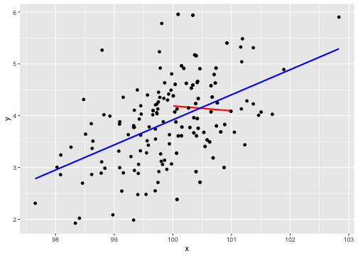<!-- --> ??? **Can you think of example where this might occur in psychology?** My idea: that many psychology studies only look at undergraduates (restricted age, restricted education) -- can't use these as predictors or covariates --- ## Nonlinearity ```r data %>% ggplot(aes(x=x, y=y)) + geom_point() + geom_smooth(method = "lm", se = FALSE, color = "red") ``` ``` ## `geom_smooth()` using formula 'y ~ x' ``` 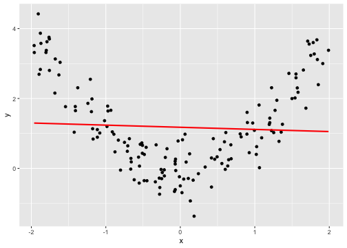<!-- --> --- ## It's not always apparent Sometimes issues that affect correlations won't appear in your graph, but you still need to know how to look for them. - Low reliability - Content overlap - Multiple groups --- ## Reliability Recall from last week: `$$r_{xy} = \rho_{xy}\sqrt{r_{xx}r_{yy}}$$` Meaning that our estimate of the population correlation coefficient is attenuated in proportion to reduction in reliability. **If you have a bad measure of X or Y, you will have a lower estimate of `\(\rho\)`.** --- ## Content overlap If your Operation Y of Construct B includes items (or tasks or manipulations) that could also be influenced by Constrct A, then the correlation between X and Y will be inflated. - Example: SAT scores and IQ tests - Example: Depression and number of hours sleeping - Which kind of validity is this associated with? --- ## Multiple groups ```r data %>% ggplot(aes(x=x, y=y)) + geom_point() + geom_smooth(method = "lm", se = FALSE, color = "red") ``` ``` ## `geom_smooth()` using formula 'y ~ x' ``` 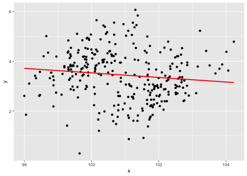<!-- --> --- ## Multiple groups ```r data %>% ggplot(aes(x=x, y=y, color = gender)) + geom_point() + geom_smooth(method = "lm", se = FALSE) + guides(color = F) ``` ``` ## `geom_smooth()` using formula 'y ~ x' ``` 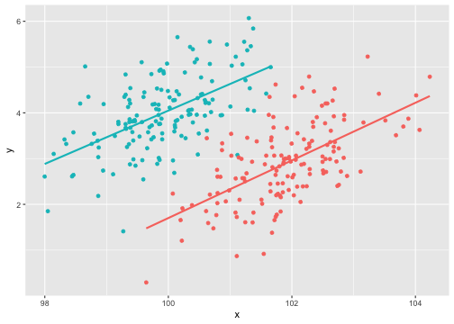<!-- --> --- ### Special cases of the Pearson correlation - **Spearman correlation coefficient** - Applies when both X and Y are ranks (ordinal data) instead of continuous - Denoted `\(\rho\)` by your textbook, although I prefer to save Greek letters for population parameters. - **Point-biserial correlation coefficient** - Applies when Y is binary. - NOTE: This is not an appropriate statistic when you [artificially dichotomize data](../readings/Cohen_1983.pdf). - **Phi ( `\(\phi\)` ) coefficient** - Both X and Y are dichotomous. --- ## Do the special cases matter? For Spearman, you'll get a different answer. ```r x = rnorm(n = 10); y = rnorm(n = 10) #randomly generate 10 numbers from normal distribution ``` .pull-left[ ```r head(cbind(x,y)) ``` ``` ## x y ## [1,] -0.6682733 -0.3940594 ## [2,] -1.7517951 0.9581278 ## [3,] 0.6142317 0.8819954 ## [4,] -0.9365643 -1.7716136 ## [5,] -2.1505726 -1.4557637 ## [6,] -0.3593537 -1.2175787 ``` ```r cor(x,y, method = "pearson") ``` ``` ## [1] 0.2702894 ``` ] .pull-right[ ```r head(cbind(x,y, rank(x), rank(y))) ``` ``` ## x y ## [1,] -0.6682733 -0.3940594 5 7 ## [2,] -1.7517951 0.9581278 2 9 ## [3,] 0.6142317 0.8819954 10 8 ## [4,] -0.9365643 -1.7716136 4 3 ## [5,] -2.1505726 -1.4557637 1 4 ## [6,] -0.3593537 -1.2175787 7 6 ``` ```r cor(x,y, method = "spearman") ``` ``` ## [1] 0.3454545 ``` ] --- ## Do the special cases matter? If your data are naturally binary, no difference between Pearson and point-biserial. ```r x = rnorm(n = 10); y = rbinom(n = 10, size = 1, prob = .3) head(cbind(x,y)) ``` ``` ## x y ## [1,] -0.48974849 1 ## [2,] -2.53667101 0 ## [3,] 0.03521883 1 ## [4,] 0.03043436 0 ## [5,] -0.27043857 0 ## [6,] -0.55228283 1 ``` .pull-left[ ```r cor(x,y, method = "pearson") ``` ``` ## [1] 0.1079188 ``` ] .pull-right[ ```r ltm::biserial.cor(x,y) ``` ``` ## [1] -0.1079188 ``` ] --- ## Do the special cases matter? If your data are artifically binary, there can be big differences. ```r x = rnorm(n = 10); y = rnorm(n = 10) ``` .pull-left[ ```r head(cbind(x,y)) ``` ``` ## x y ## [1,] 1.27516603 -0.2012149 ## [2,] -1.55729177 0.2925842 ## [3,] 0.09364959 0.0821713 ## [4,] 0.87343693 0.1879078 ## [5,] 0.74807054 0.3794815 ## [6,] 0.02831971 -1.2940189 ``` ```r cor(x,y, method = "pearson") ``` ``` ## [1] -0.1584301 ``` ] .pull-right[ ```r d_y = ifelse(y < median(y), 0, 1) head(cbind(x,y, d_y)) ``` ``` ## x y d_y ## [1,] 1.27516603 -0.2012149 0 ## [2,] -1.55729177 0.2925842 1 ## [3,] 0.09364959 0.0821713 0 ## [4,] 0.87343693 0.1879078 0 ## [5,] 0.74807054 0.3794815 1 ## [6,] 0.02831971 -1.2940189 0 ``` ```r ltm::biserial.cor(x,d_y) ``` ``` ## [1] 0.4079477 ``` ] ### Don't use median splits! --- ### Special cases of the Pearson correlation Why do we have special cases of the correlation? - Sometimes we get different results - If we treat ordinal data like interval/ratio data, our estimate will be incorrect - Sometimes we get the same result - Even when formulas are different - Example: Point biserial formula - `$$r_{pb} = \frac{M_1-M_0}{\sqrt{\frac{1}{n-1}\Sigma(X_i-\bar{X})^2}}\sqrt{\frac{n_1n_0}{n(n-1)}}$$` ??? We don't have different formulas because the correlation is mathematically different -- these formulas were developed when we did things by hand. These formulas are short cuts! --- class: inverse ## Next time... matrix algebra