class: center, middle, inverse, title-slide # Comparing two means: effect sizes and assumptions --- ## Reminders * Quiz 9 is on Thursday next week * Homework 3 due next Friday, but grading starts this weekend * Please fill out the End-of-Course Student Experience Survey (available in DuckWeb) * Psych Twitter talked about [effect sizes](https://twitter.com/farid_anvari/status/1332745933860298754) over the [weekend](https://twitter.com/BrentWRoberts/status/1332769974201569281?s=20). --- ## Last time * Introduction to independent samples *t*-tests * Standard error of the **difference of means** * Pooled variance, `\(\hat{\sigma}_P\)` * Confidence intervals around the difference in means * Confidence intervals around different means --- ## Review of independent samples *t*-tests It's generally argued that Republicans have an age problem -- but are they substantially older than Democrats? In 2014 (midterm election before the most recent presidential election), [*Five Thirty Eight* did an analysis](https://fivethirtyeight.com/features/both-republicans-and-democrats-have-an-age-problem/) of the ages of elected members of Congress. They've provided their data, so we can run analyses on our own. ```r library(fivethirtyeight) ``` --- ```r congress = congress_age %>% filter(congress == 113) %>% # just the most recent filter(party %in% c("R", "D")) # remove independents ``` ```r psych::describe(congress$age) ``` ``` ## vars n mean sd median trimmed mad min max range skew kurtosis se ## X1 1 542 57.58 10.92 57.95 57.66 10.82 29.8 93 63.2 -0.02 -0.13 0.47 ``` --- ```r congress %>% ggplot(aes(x = age)) + geom_histogram(bins = 50, color = "white") + labs(x = "Age in years", y = "Frequency", title = "Age Distribution of Congressional \nMembers in 113th Congress", caption = "This is pretty normal.") + theme_bw(base_size = 20) ``` <!-- --> --- ```r congress %>% ggplot(aes(x = age, fill = party)) + geom_histogram(bins = 50, color = "white", position = "dodge") + labs(x = "Age in years", y = "Frequency", title = "Age Distribution of Congressional \nMembers in 113th Congress", caption = "This is pretty normal.") + scale_fill_manual(values = c("blue", "red")) + theme_bw(base_size = 20) ``` <!-- --> --- ```r psych::describeBy(congress$age, group = congress$party) ``` ``` ## ## Descriptive statistics by group ## group: D ## vars n mean sd median trimmed mad min max range skew kurtosis se ## X1 1 259 59.55 10.85 60.4 59.85 10.53 29.8 93 63.2 -0.19 0.02 0.67 ## ------------------------------------------------------------ ## group: R ## vars n mean sd median trimmed mad min max range skew kurtosis se ## X1 1 283 55.78 10.68 56.1 55.67 9.79 31.6 89.7 58.1 0.13 -0.11 0.64 ``` .pull-left[ $$ `\begin{aligned} \bar{X}_1 &= 59.55 \\ \hat{\sigma}_1 &= 10.85 \\ N_1 &= 259 \\ \end{aligned}` $$ ] .pull-right[ $$ `\begin{aligned} \bar{X}_2 &= 55.78 \\ \hat{\sigma}_2 &= 10.68 \\ N_2 &= 283 \\ \end{aligned}` $$ ] --- Next we build the sampling distribution under the null hypotheses. $$ `\begin{aligned} \mu &= 0 \\ \\ \sigma_D &= \sqrt{\frac{(259-1){10.85}^2 + (283-1){10.68}^2}{259+283-2}} \sqrt{\frac{1}{259} + \frac{1}{283}}\\ &= 10.76\sqrt{\frac{1}{259} + \frac{1}{283}} = 0.93\\ \\ df &= 540 \end{aligned}` $$ --- ``` ## [1] 1.964367 ``` ```r (t = (x1-x2)/s_d) ``` ``` ## [1] 4.071568 ``` <!-- --> --- ```r library(ggpubr) ggerrorplot(congress, x = "party", y = "age", desc_stat = "mean_ci", xlab = "Party", ylab = "Average Age", color = "party", palette = c("red", "blue")) ``` <!-- --> --- ```r ggerrorplot(congress, x = "party", y = "age", desc_stat = "mean_ci", xlab = "Party", ylab = "Average Age", color = "party", palette = c("red", "blue"), add = "violin") + stat_compare_means(comparisons =list(c("R", "D"))) ``` 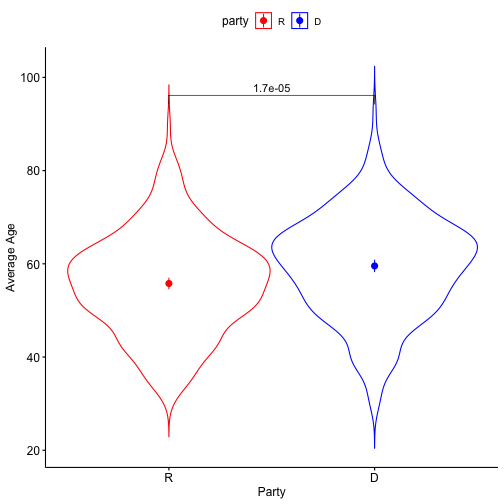<!-- --> --- ### A difference in significance is not a significant difference Researchers commonly examine effects within separate groups. This can be an appropriate strategy, especially if there is reason to think that the mechanisms linking X to Y differ by groups. For example, traditional benchmarks might suggest that the average young adult reports a stress-level of 3.4 out of 5. But these benchmarks are estimated from a population of white young adults; you conduct a study looking at young Hispanic adults and young African American adults. .pull-left[ `$$\bar{X}_H: 3.55$$` `$$s_H: 0.739$$` `$$N_H: 36$$` ] .pull-left[ `$$\bar{X}_B: 3.7$$` `$$s_B: 0.788$$` `$$N_B: 62$$` ] --- We can plot these effects against our population mean: 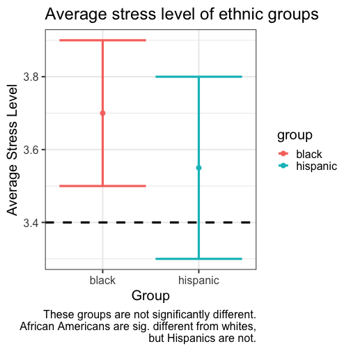<!-- --> ??? These groups are not significantly different from each other. Just because one group is sig and the other is not, doesn't mean they are different. This expands beyond one-sample t-tests. For example, if there is a sig. correlation in one group but not another, or a sig ANOVA, or a sig whatever; you have to formally test to say two groups are different. --- ## Effect sizes Cohen suggested one of the most common effect size estimates—the standardized mean difference—useful when comparing a group mean to a population mean or two group means to each other. This is referred to as **Cohen's d**. `$$\delta = \frac{\mu_1 - \mu_0}{\sigma} \approx d = \frac{\bar{X}_1-\bar{X}_2}{\hat{\sigma}_p}$$` -- Cohen’s d is in the standard deviation (Z) metric. What happens to Cohen's d as sample size gets larger? --- Let's go back to our politics example: .pull-left[ **Democrats** $$ `\begin{aligned} \bar{X}_1 &= 59.55 \\ \hat{\sigma}_1 &= 10.85 \\ N_1 &= 259 \\ \end{aligned}` $$ ] .pull-right[ **Republicans** $$ `\begin{aligned} \bar{X}_2 &= 55.78 \\ \hat{\sigma}_2 &= 10.68 \\ N_2 &= 283 \\ \end{aligned}` $$ ] `$$\hat{\sigma}_p = \sqrt{\frac{(259-1){10.85}^2 + (283-1){10.68}^2}{259+283-2}} = 10.76$$` `$$d = \frac{59.55-55.78}{10.76} = 0.35$$` How do we interpret this? Is this a large effect? --- Cohen (1988) suggests the following guidelines for interpreting the size of d: .large[ - .2 = Small - .5 = Medium - .8 = Large ] An aside, to calculate Cohen's D for a one-sample *t*-test: `$$d = \frac{\bar{X}-\mu}{\hat{\sigma}}$$` .small[Cohen, J. (1988), Statistical power analysis for the behavioral sciences (2nd Ed.). Hillsdale: Lawrence Erlbaum.] --- Another useful metric is the overlap between the two population distributions -- the smaller the overlap, the farther apart the distributions. As a reminder, our data constitutes only samples representing the larger populations, so we use our statistics to build estimated population distributions. --- 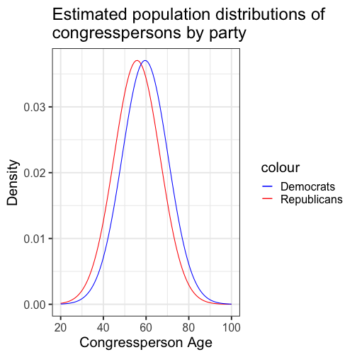<!-- --> --- 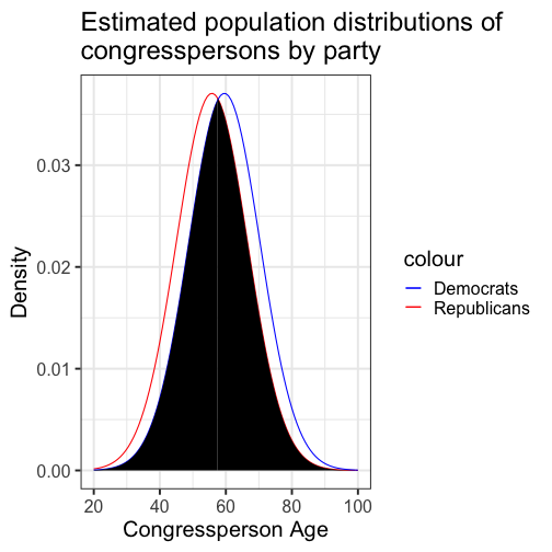<!-- --> These distributions have 86.1 % overlap. --- ### Calculation of distribution overlap There is a straightforward relationship between Cohen's d and distribution overlap: `$$\text{Overlap} = P(X \leq -\frac{|d|}{2})*2$$` ```r 2 * pnorm(-abs(0.35)/2) ``` ``` ## [1] 0.8610796 ``` --- ## Cohen's D (Paired-samples _t_) Recall our gull example from the paired-samples _t_-test lecture. The average difference in seconds was `\(83.11 (SD = 115.85)\)`. ```r t.test(gulls$At, gulls$Away, paired = T) ``` ``` ## ## Paired t-test ## ## data: gulls$At and gulls$Away ## t = 3.1269, df = 18, p-value = 0.005826 ## alternative hypothesis: true difference in means is not equal to 0 ## 95 percent confidence interval: ## 27.26807 138.94246 ## sample estimates: ## mean of the differences ## 83.10526 ``` --- Calculating a standardized effect size for a paired samples t-test (and research design that includes nesting or dependency) is slightly complicated, because there are two levels at which you can describe results. The first level is the **within-subject** (or within-pair, or within-gull) level, and this communicates effect size in the unit of differences (of units). `$$d = \frac{\bar{\Delta}}{\hat{\sigma_\Delta}} = \frac{83.11}{115.85} = 0.72$$` The interpretation is that, on average, variability within a single gull is about .72 standard deviations of differences of seconds. --- ### Cohen's D (Paired-samples _t_) ```r lsr::cohensD(x = gulls$At, y = gulls$Away, method = "paired") ``` ``` ## [1] 0.7173615 ``` The second level is the **between-conditions** variance, which is in the units of your original outcome and communicates how the means of the two conditions differ. For that, you can use the Cohen's d calculated for independent samples *t*-tests. ```r lsr::cohensD(x = gulls$At, y = gulls$Away, method = "pooled") ``` ``` ## [1] 0.8137369 ``` --- **Which one should you use?** The first thing to recognize is that, unlike hypothesis testing, there are no standards for effect sizes. When Cohen developed his formula in 1988, he never bothered to precisely define `\(\large \sigma\)`. Interpretations have varied, but no single method for within-subjects designs has been identified. Most often, textbooks will argue for the within-pairs version, because this mirrors the hypothesis test. Some (see below) argue the between-conditions version is actually better because the paired-design is used to reduce noise by adjusting our calculation of the standard error. But that shouldn't make our effect bigger, just easier to detect. The other argument is that using the same formula (the between-conditions version) allows us to compare effect sizes across many different designs, which are all trying to capture the same effect. .small[Westfall, J. (2016). [Five different "Cohen's d" statistics for within-subject designs](http://jakewestfall.org/blog/index.php/2016/03/25/five-different-cohens-d-statistics-for-within-subject-designs/)] --- ### Cohen's D from *t* This can be calculating from *t*-statistics, allowing you to calculate standardized effect sizes from manuscripts even when the authors did not provide them. .pull-left[ **One sample or within-subjects for paired** `$$\large d = \frac{t}{\sqrt{N-1}}$$` ] .pull-right[**Independent sample** `$$\large d = \frac{2t}{\sqrt{N_1+N_2-1}}$$` ] --- ## When should you not use Student's *t*-test? Recall the three assumptions of Student's *t*-test: * Independence * Normality * Homogeneity of variance There are no good statistical tests to determine whether you've violated the first -- it depends on how you sampled your population. -- * Draw phone numbers at random from a phone book? * Recruit random sets of fraternal twins? * Randomly select houses in a city and interview the person who answers the door? --- ### Homogeneity of variance Homogeneity of variance can be checked with Levene’s procedure. It tests the null hypothesis that the variances for two or more groups are equal (or within sampling variability of each other): `$$H_0: \sigma^2_1 = \sigma^2_2$$` `$$H_0: \sigma^2_1 \neq \sigma^2_2$$` Levene's test can be expanded to more than two variances; in this case, the alternative hypothesis is that at least one variance is different from at least one other variance. Levene's produces a statistic, *W*, that is *F* distributed with degrees of freedom of `\(k-1\)` and `\(N-k\)`. --- ```r library(car) leveneTest(age~party, data = congress, center = "mean") ``` ``` ## Levene's Test for Homogeneity of Variance (center = "mean") ## Df F value Pr(>F) ## group 1 0.0663 0.797 ## 540 ``` Like other tests of significance, Levene’s test gets more powerful as sample size increases. So unless your two variances are *exactly* equal to each other (and if they are, you don't need to do a test), your test will be "significant" with a large enough sample. Part of the analysis has to be an eyeball test -- is this "significant" because they are truly different, or because I have many subjects. --- ### Homogeneity of variance The homogeneity assumption is often the hardest to justify, empirically or conceptually. If we suspect the means for the two groups could be different (H1), that might extend to their variances as well. Treatments that alter the means for the groups could also alter the variances for the groups. Welch’s *t*-test removes the homogeneity requirement, but uses a different calculation for the standard error of the mean difference and the degrees of freedom. One way to think about the Welch test is that it is a penalized *t*-test, with the penalty imposed on the degrees of freedom in relation to violation of variance homogeneity (and differences in sample size). --- ### Welch's *t*-test `$$t = \frac{\bar{X}_1-\bar{X_2}}{\sqrt{\frac{\hat{\sigma}^2_1}{N_1}+\frac{\hat{\sigma}^2_2}{N_2}}}$$` So that's a bit different -- the main difference here is the way that we weight sample variances. It's true that larger samples still get more weight, but not as much as in Student's version. Also, we divide variances here by N instead of N-1, making our standard error larger. ??? ### Don't go into the weighting of variances thing -- too confusing --- ### Welch's *t*-test The degrees of freedom are different: `$$df = \frac{[\frac{\hat{\sigma}^2_1}{N_1}+\frac{\hat{\sigma}^2_2}{N_2}]^2}{\frac{[\frac{\hat{\sigma}^2_1}{N1}]^2}{N_1-1}+\frac{[\frac{\hat{\sigma}^2_2}{N2}]^2}{N_2-1}}$$` These degrees of freedom can be fractional. As the sample variances converge to equality, these df approach those for Student’s *t*, for equal N. --- ```r t.test(age~party, data = congress, var.equal = F) ``` ``` ## ## Welch Two Sample t-test ## ## data: age by party ## t = 4.0688, df = 534.2, p-value = 5.439e-05 ## alternative hypothesis: true difference in means is not equal to 0 ## 95 percent confidence interval: ## 1.949133 5.588133 ## sample estimates: ## mean in group D mean in group R ## 59.55097 55.78233 ``` --- ### Normality Finally, there's the assumption of normality. Specifically, this is the assumption that the population is normal -- if the population is normal, then our sampling distribution is **definitely** normal and we can use a *t*-distribution. But even if the population is not normal, the CLT lets us assume our sampling distribution is normal because as N approaches infinity, the sampling distributions approaches normality. So we can be **pretty sure** the sampling distribution is normal. One thing we can check -- the only distribution we actually have access to -- is the sample distribution. If this is normal, then we can again be pretty sure that our population distribution is normal, and thus our sampling distribution is normal too. --- Normality can be checked with a formal test: the Shapiro-Wilk test. The test statistic, W, has an expected value of 1 under the null hypothesis. Departures from normality reduce the size of W. A statistically significant W is a signal that the sample distribution departs significantly from normal. But... * With large samples, even trivial departures will be statistically significant. * With large samples, the sampling distribution of the mean(s) will approach normality, unless the data are very non-normally distributed. * Visual inspection of the data can confirm if the latter is a problem. * Visual inspection can also identify outliers that might influence the data. --- ```r shapiro.test(x = congress$age) ``` ``` ## ## Shapiro-Wilk normality test ## ## data: congress$age ## W = 0.99663, p-value = 0.3168 ``` ```r hist(congress$age, col = "purple", border = "white") ``` <!-- --> --- A common non-parametric test that can be used in place of the independent samples *t*-test is the **Wilcoxon sum rank test**. Here's the calculation: * Order all the data points by their outcome. * For one of the groups, add up all the ranks. That's your test statistic, *W*. * To build the sampling distribution, randomly shuffle the group labels and add up the ranks for your group of interest again. Repeat this process until you've calculated the rank sum for every possible group assignment. ```r wilcox.test(age~party, data = congress) ``` ``` ## ## Wilcoxon rank sum test with continuity correction ## ## data: age by party ## W = 44488, p-value = 1.674e-05 ## alternative hypothesis: true location shift is not equal to 0 ``` --- class: inverse ## Next time... matrix algebra of t-tests and wrap up! Plus the final quiz