t-tests: one-sample and paired

class: center, middle, inverse, title-slide

# <em>t</em>-tests: one-sample and paired

---

## Previously...

* chi-square `$(\chi^2) tests$`

---

### Today

* One-sample _t_-tests
* Paired-samples _t_-tests

---

When we move from categorical outcomes to variables measured on an interval or ratio scale, we become interested in means rather than frequencies.  Comparing means is usually done with the *t*-test, of which there are several forms.

The one-sample *t*-test is appropriate when a single sample mean is compared to a population mean but the population standard deviation is unknown.  A sample estimate of the population standard deviation is used instead.  The appropriate sampling distribution is the t-distribution, with N-1 degrees of freedom.

`$$t_{df=N-1} = \frac{\bar{X}-\mu}{\frac{\hat{\sigma}}{\sqrt{N}}}$$`
The heavier tails of the t-distribution, especially for small N, are the penalty we pay for having to estimate the population standard deviation from the sample.

---

### One-sample *t*-tests

*t*-tests were developed by William Sealy Gosset, who was a chemist studying the grains used in making beer. (He worked for Guinness.)

* Specifically, he wanted to know whether particular strains of grain made better or worse beer than the standard.

* He developed the *t*-test, to test small samples of beer against a population with an unknown standard deviation.
  
  * Probably had input from Karl Pearson and Ronald Fisher
  
* Published this as "Student" because Guinness didn't want these tests tied to the production of beer.

---

### One-sample *t*-tests

We've already been covering one-sample *t*-tests, but let's formally walk through some of the steps and how this differs from a z-test.

| | Z-test | *t*-test |
| --|--------|--------|
| `$\large{\mu}$` | known | known |
| `$\sigma$` | known |unknown |
| sem or `$\sigma_M$` | `$\frac{\sigma}{\sqrt{N}}$` | `$\frac{\hat{\sigma}}{\sqrt{N}}$` or `$\frac{s}{\sqrt{N}}$`|
|Probability distribution | standard normal | `$t$` |
| DF | none | `$N-1$` |
| Tails | One or two | One or two |
| Critical value ( `$\alpha = .05$` two-tailed) | 1.96 | Depends on DF |

---

### When you assume...

...you can run a parametric statistical test!

**Assumptions of the one-sample *t*-test**

**Normality.** We assume the sampling distribution of the mean is normally distributed. How can we make this assumption?

**Independence.** Observations in the dataset are not associated with one another. Put another way, collecting a score from Participant A doesn't tell me anything about what Participant B will say. How can we be safe in this assumption?

---

### A brief example

Using the same Census at School data, we find that Oregon students who participated in a memory game ( `$N = 197$` ) completed the game in an average time of `$49.13$` seconds `$(s = 13.42)$`. We know that the average US student completed the game in 45.04 seconds. How do our students compare?

**Hypotheses**

`$H_0: \mu = 45.05$`

`$H_1: \mu \neq 45.05$`

???

`$sem = 0.9562$`
`$t = 4.2652$`
`$p1 = 0.0000155$`
`$p = 0.000031$`

---

```r
t.test(x = school$Score_in_memory_game, mu = 45.05, 
       alternative = "two.sided")
```

```
## 
## 	One Sample t-test
## 
## data:  school$Score_in_memory_game
## t = 4.2652, df = 196, p-value = 0.00003104
## alternative hypothesis: true mean is not equal to 45.05
## 95 percent confidence interval:
##  47.24269 51.01427
## sample estimates:
## mean of x 
##  49.12848
```

---

```r
lsr::oneSampleTTest(x = school$Score_in_memory_game, 
                    mu = 45.05, one.sided = FALSE)
```

```
## 
##    One sample t-test 
## 
## Data variable:   school$Score_in_memory_game 
## 
## Descriptive statistics: 
##             Score_in_memory_game
##    mean                   49.128
##    std dev.               13.421
## 
## Hypotheses: 
##    null:        population mean equals 45.05 
##    alternative: population mean not equal to 45.05 
## 
## Test results: 
##    t-statistic:  4.265 
##    degrees of freedom:  196 
##    p-value:  <.001 
## 
## Other information: 
##    two-sided 95% confidence interval:  [47.243, 51.014] 
##    estimated effect size (Cohen's d):  0.304
```

???

Draw attention here to:

1. confidence interval -- doesn't contain null hypothesis
2. cohen's d

---
## Shifting confidence intervals

![](15-t_one_paired_files/figure-html/unnamed-chunk-4-1.gif)

---

The difference in means was 4.08. Is that big?

---
# Cohen's D

Cohen suggested one of the most common effect size estimates—the standardized mean difference—useful when comparing a group mean to a population mean or two group means to each other.

`$$\delta = \frac{\mu_1 - \mu_0}{\sigma} \approx d = \frac{\bar{X}-\mu}{\hat{\sigma}}$$`

Cohen’s d is in the standard deviation (Z) metric.

---

Cohens’s d for these data is .30.  In other words, the sample mean differs from the population mean by .30 standard deviation units.

Cohen (1988) suggests the following guidelines for interpreting the size of d:

.large[

- 	.2 = Small

- 	.5 = Medium

- 	.8 = Large

]
.small[Cohen, J. (1988), Statistical power analysis for the behavioral sciences (2nd Ed.). Hillsdale: Lawrence Erlbaum.]
---

Another useful metric is the overlap between the two distributions -- the smaller the overlap, the farther apart the distributions

![](15-t_one_paired_files/figure-html/unnamed-chunk-6-1.png)

---

### The usefulness of the one-sample *t*-test

How often will you conducted a one-sample *t*-test on raw data?

* (Probably) never

How often will you come across one-sample *t*-tests?

* (Probably) a lot!

The one-sample *t*-test is used to test coefficients in a model.

---

```r
model = lm(health ~ education, data = psychTools::spi)
summary(model)
```

```
## 
## Call:
## lm(formula = health ~ education, data = psychTools::spi)
## 
## Residuals:
##     Min      1Q  Median      3Q     Max 
## -2.6683 -0.5896  0.3317  0.5284  1.6071 
## 
## Coefficients:
##             Estimate Std. Error t value             Pr(>|t|)    
## (Intercept) 3.353512   0.036015  93.116 < 0.0000000000000002 ***
## education   0.039348   0.007732   5.089           0.00000038 ***
## ---
## Signif. codes:  0 '***' 0.001 '**' 0.01 '*' 0.05 '.' 0.1 ' ' 1
## 
## Residual standard error: 0.9733 on 3251 degrees of freedom
##   (747 observations deleted due to missingness)
## Multiple R-squared:  0.007903,	Adjusted R-squared:  0.007598 
## F-statistic:  25.9 on 1 and 3251 DF,  p-value: 0.0000003803
```

---
class:inverse

repeated measures

---

In **longitudinal research**, the same people provide responses to the same measure on two occasions (the individuals in the two groups are the same).

In **paired-sample research**, the individuals in the two groups are different, but they are related and their responses are assumed to be correlated.  Examples would be responses by children and their parents, members of couples, twins, etc.

In **paired-measures research**, the same people provide responses to two different measures that assess closely related constructs.  This resembles longitudinal research, but data collection occurs at one time.

All of these are instances of repeated measures designs.

---

The advantage of repeated measures designs is that, compared to an independent groups design of the same size, the repeated measures design is **more powerful**.

* Two groups are more alike than in simple randomization

* The correlated sampling units will have less variability on "nuisance variables" because those are either the same over time (longitudinal) or over measures (paired measures), or very similar over people (paired samples).

* Nuisance variables -- anything that isn't relevant to the study.

---

Each of these repeated measures problems can be viewed as a transformation of the original two measures into a single measure: a difference score.  This reduces the analysis to a one-sample *t*-test on the difference score, with null mean = 0.

---

If the repeated measures are `$X_1$` and `$X_2$`, then their difference is `$D = X_1 – X_2$`.  This new measure has a mean and standard deviation, like any other single measure, making it appropriate for a one-sample *t*-test.

`$$t_{df = N-1} = \frac{\bar{\Delta}-\mu}{\frac{\hat{\sigma}_\Delta}{\sqrt{N}}}$$`

.pull-left[
`$$H_0: \bar{\Delta} = \mu$$`
`$$H_1: \bar{\Delta} \neq \mu$$`
]

.pull-right[
`$$H_0: \bar{\Delta} = 0$$`
`$$H_1: \bar{\Delta} \neq 0$$`
]

???
Note here the signal to noise ratios

---

## Example

Human-wildlife conflict in urban areas endangers wildlife species. One species under threat is the *Larus argentatus* or herring gull, which is considered a nuisance owing to food-snatching and other behaviors. A [recent study](https://royalsocietypublishing.org/doi/10.1098/rsbl.2019.0405) examined whether herring gull behavior is influenced by human behavior cues and whether this could be used to reduce human-gull conflict.

.pull-left[
![](images/gulls.jpg)]

.pull-right[
In this study, experimenters visited coastal towns in the UK and found locations with multiple gulls. They placed a bag of potato chips (250 g) in front of them and measured how long it took gulls to peck at the food. 
]

---
.pull-left[

![](images/gulls_at.jpg)

In the **Looking At** treatment, the experimenter directed her gaze towards the eye(s) of the gull and turned her head, if necessary, to follow its approach path until the gull completed the trial by pecking at the food bag. 
]

.pull-right[

![](images/gulls_away.jpg)

In the **Looking Away** treatment, the experimenter turned her head and eyes approximately 60° (randomly left or right) away from the gull and maintained this position until she heard the gull peck at the food bag. 
]

"We adopted a repeated measures design... We randomly assigned individuals to receive Looking At or Looking Away first, and trial order was counterbalanced across individuals. Second trials commenced 180 s after the completion of the first trial to allow normal behaviour to resume."

---

```r
gulls = read.delim(here("data/gulls/pairs.txt"))
gulls
```

```
##    GullID  At Away
## 1   FAL01 210   35
## 2   FAL03 300   80
## 3   FAL04   6    3
## 4   PEN03  18   21
## 5   W120M  47   13
## 6    W019  25    4
## 7   PNZ01   4   13
## 8   PNZ02   9    8
## 9   STI01 300   18
## 10  STI02 300    6
## 11   W186  11    8
## 12  STI03   4    3
## 13  STI04   4    6
## 14  HEL02  12   19
## 15  NEW01 300    6
## 16  NEW02  63   16
## 17  NEW03 300  166
## 18  PER01  24   66
## 19  TRU01 300  167
```

???

FAL = Falmouth
PEN = Penryn

---

### Hypothesis testing

Use a paired-samples *t*-test because we have the same gulls in both conditions.

`$\large H_0$`: There is no difference in how long it takes gulls to approach food between conditions.

`$\large H_1$`: Gulls take longer to approach food in one of the conditions.

---

### Sampling distribution

*t*-distribution requires two parameters, a mean and a standard deviation.

The mean of our sampling distribution comes from our null hypothesis, so

`$$\large \mu = 0$$`

Our standard deviation of our sampling distribution is the **standard error of difference scores**. This can be found by
  1. calculating difference scores
  2. calculating the standard deviation of the difference scores, and 
  3. dividing the standard deviation by the square root of the number of *pairs* in your study.
  
---

```r
difference = gulls$At - gulls$Away
```

```
## [1] 175 220   3  -3  34  21
```

.pull-left[
We can take the mean of this new variable:

```r
(m_delta = mean(difference))
```

```
## [1] 83.10526
```

]

--
.pull-right[

And we can calculate the standard deviation

```r
(s_delta = sd(difference))
```

```
## [1] 115.8485
```

]

To calculate the standard error of difference scores, we simply divide the standard deviation by the square root of the number of *pairs* or, if repeated measures, the number of *subjects*.

```r
(se_delta = s_delta/sqrt(nrow(gulls)))
```

```
## [1] 26.57747
```

`$$\frac{\hat{\sigma}_\Delta}{\sqrt{N}} = 26.58$$`
---

![](15-t_one_paired_files/figure-html/unnamed-chunk-13-1.png)

---

### Test statistic

`$$t_{df = N-1} = \frac{\bar{\Delta}-\mu}{\frac{\hat{\sigma}_\Delta}{\sqrt{N}}}$$`

In this case, N refers to the number of pairs, not the total sample size.

`$$t_{df = N-1} = \frac{83.11-0}{26.58} = 3.13$$`

**Note:** A paired-samples *t*-test is *exactly* the same as a one-sample *t*-test on the difference scores.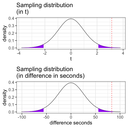

---

![](15-t_one_paired_files/figure-html/unnamed-chunk-14-1.png)

---

Another option is to calculate the area above the absolute value of the test statistic and multiply that by two -- this estimates the probability of finding this test statistic or more extreme.

```r
(t_statistic = m_delta/se_delta)
```

```
## [1] 3.126906
```

```r
pt(t_statistic, df = 19-1, lower.tail = F)
```

```
## [1] 0.002912942
```

```r
pt(t_statistic, df = 19-1, lower.tail = F)*2
```

```
## [1] 0.005825884
```

---
## t-test functions

```r
t.test(x = gulls$At, y = gulls$Away, 
       paired = TRUE)
```

```
## 
## 	Paired t-test
## 
## data:  gulls$At and gulls$Away
## t = 3.1269, df = 18, p-value = 0.005826
## alternative hypothesis: true difference in means is not equal to 0
## 95 percent confidence interval:
##   27.26807 138.94246
## sample estimates:
## mean of the differences 
##                83.10526
```

---

```r
ggpubr::ggpaired(data = gulls, cond1 = "At", cond2 = "Away", line.color = "grey",
                 ylab = "Time to approach (seconds)", 
                 title = "Some gulls approach food more quickly when \npeople look away from them")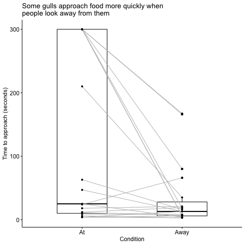
```

![](15-t_one_paired_files/figure-html/unnamed-chunk-17-1.png)

---

## The variance of difference scores

With the raw data, the calculation of the variance of the standard deviation scores `$\large (\hat{\sigma}_\Delta)$` is intuitive. Sometimes you will not have access to the raw data, but will want to conduct the test.

For example, you read a study that compares a sample of Oregon students to known US benchmarks on several variables using multiple one-sample *t*-tests; you want to know whether OR students respond more to one variable than the other.

<table class="table" style="margin-left: auto; margin-right: auto;">
 <thead>
  <tr>
   <th style="text-align:left;">   </th>
   <th style="text-align:right;"> N </th>
   <th style="text-align:right;"> Mean </th>
   <th style="text-align:right;"> SD </th>
  </tr>
 </thead>
<tbody>
  <tr>
   <td style="text-align:left;"> Importance_reducing_pollution </td>
   <td style="text-align:right;"> 194 </td>
   <td style="text-align:right;"> 792.15 </td>
   <td style="text-align:right;"> 937.03 </td>
  </tr>
  <tr>
   <td style="text-align:left;"> Importance_recycling_rubbish </td>
   <td style="text-align:right;"> 194 </td>
   <td style="text-align:right;"> 714.85 </td>
   <td style="text-align:right;"> 652.65 </td>
  </tr>
</tbody>
</table>

The correlation between these variables is 0.61.

---

It turns out that the mean difference score is the same as the difference in means, so that's an easy part of the calculation.

But the calculation of the standard deviation becomes a little more complicated:

`$$\large \hat{\sigma}_\Delta = \sqrt{\hat{\sigma}^2_{X_1} + \hat{\sigma}^2_{X_2} - 2r(\hat{\sigma}_{X_1}\hat{\sigma}_{X_2})}$$`

```r
sd_1 = 937.03
sd_2 = 652.65
cor_12 = .61
var_d = sd_1^2 + sd_2^2 -2*cor_12*sd_1*sd_2
sqrt(var_d)
```

```
## [1] 746.9157
```

---

Now you have all the information you need for the statistical test!

```r
(t = (792.15-714.85)/(746.92/sqrt(194)))
```

```
## [1] 1.441472
```

```r
pt(t, df = 193, lower.tail = F)*2
```

```
## [1] 0.1510719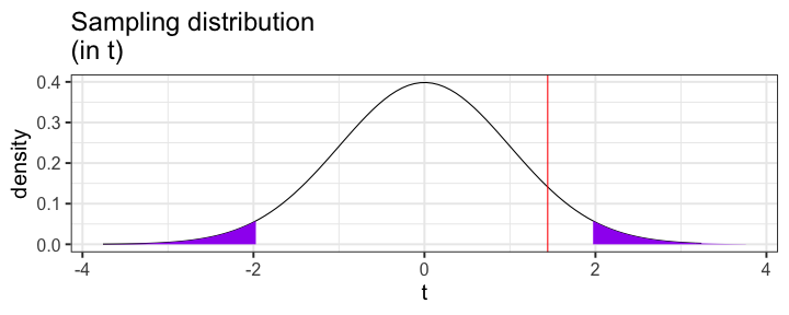
```

![](15-t_one_paired_files/figure-html/unnamed-chunk-22-1.png)

???

Useful for meta-analysis or getting more information from articles you read.

What else can this equation tell us?

* What happens if the two variables are highly correlated with each other?

---

`$$\large \hat{\sigma}_\Delta = \sqrt{\hat{\sigma}^2_{X_1} + \hat{\sigma}^2_{X_2} - 2r(\hat{\sigma}_{X_1}\hat{\sigma}_{X_2})}$$`

What happens if `$\large r$` is large and positive?

What happens if `$\large r$` is small and positive?

What happens if `$\large r$` is negative?

???

large and postive: se is very small
small and positive: se is smaller but not so much
negative: se is bigger

take away: likely to find differences when two measures are positively associated, but hurt if negatively
may consider reverse scoring measures...

---

## Assumptions

* Independence (between pairs)
* Normality

**Note:** These are the same assumptions as a one-sample *t*-test.

---

class: inverse

### Next time...

* Independent samples _t_-tests