Describing Data II
Announcements
Homework 1 due in < two weeks
Measure yourself for an in-class demo today tinyurl.com/uwn463vj
- height (inches)
- length of right forearm (inches)
Population variability
Sums of squares
\[ \small SS = \Sigma(X_i-\bar{X})^2 \]
Variance
\[ \small \sigma^2 = \frac{\Sigma(X_i-\bar{X})^2}{N} = \frac{SS}{N} \]
Standard deviation
\[ \scriptsize \sigma = \sqrt{\frac{\Sigma(X_i-\bar{X})^2}{N}}= \sqrt{\frac{SS}{N}} = \sqrt{\sigma^2} \]
Sample variability
Sums of squares
\[ \small SS = \Sigma(X_i-\bar{X})^2 \]
Variance
\[ \small \hat{\sigma}^2 = s^2 = \frac{\Sigma(X_i-\bar{X})^2}{N-1} = \frac{SS}{N-1} \]
Standard deviation
\[ \scriptsize \hat{\sigma} = s = \sqrt{\frac{\Sigma(X_i-\bar{X})^2}{N-1}}= \sqrt{\frac{SS}{N-1}} = \sqrt{s^2} \]
Bi-variate descriptives
Covariation
“Sum of the cross-products”
Population
\[SP_{XY} =\Sigma(X_i−\mu_X)(Y_i−\mu_Y)\]
Sample
\[ SP_{XY} =\Sigma(X_i−\bar{X})(Y_i−\bar{Y})\]
Covariance
Sort of like the variance of two variables
Population
\[\sigma_{XY} =\frac{\Sigma(X_i−\mu_X)(Y_i−\mu_Y)}{N}\]
Sample
\[s_{XY} = cov_{XY} =\frac{\Sigma(X_i−\bar{X})(Y_i−\bar{Y})}{N-1}\]
Covariance table
\[\Large \mathbf{K_{XX}} = \left[\begin{array} {rrr} \sigma^2_X & cov_{XY} & cov_{XZ} \\ cov_{YX} & \sigma^2_Y & cov_{YZ} \\ cov_{ZX} & cov_{ZY} & \sigma^2_Z \end{array}\right]\]
Correlation
Measure of association
How much two variables are linearly related
-1 to 1
Sign indicates direction of relationship
Invariant to changes in mean or scaling
Correlation
Pearson product moment correlation
Population
\[\rho_{XY} = \frac{\Sigma z_Xz_Y}{N} = \frac{SP}{\sqrt{SS_X}\sqrt{SS_Y}} = \frac{\sigma_{XY}}{\sigma_X \sigma_Y}\]
Sample \[r_{XY} = \frac{\Sigma z_Xz_Y}{n-1} = \frac{SP}{\sqrt{SS_X}\sqrt{SS_Y}} = \frac{s_{XY}}{s_X s_Y}\]
Code
set.seed(101019) # so we all get the same random numbers
mu = c(50, 5) # means of two variables (MX = 50, MY = 5)
Sigma = matrix(c(.8, .5, .5, .7), ncol =2) #diagonals are reliabilites, off-diagonals are correlations
data = mvrnorm(n = 150, mu = mu, Sigma = Sigma)
data = as.data.frame(data)
colnames(data) = c("x", "y")
data %>% ggplot(aes(x = x, y = y)) + geom_point(size = 3) + theme_bw()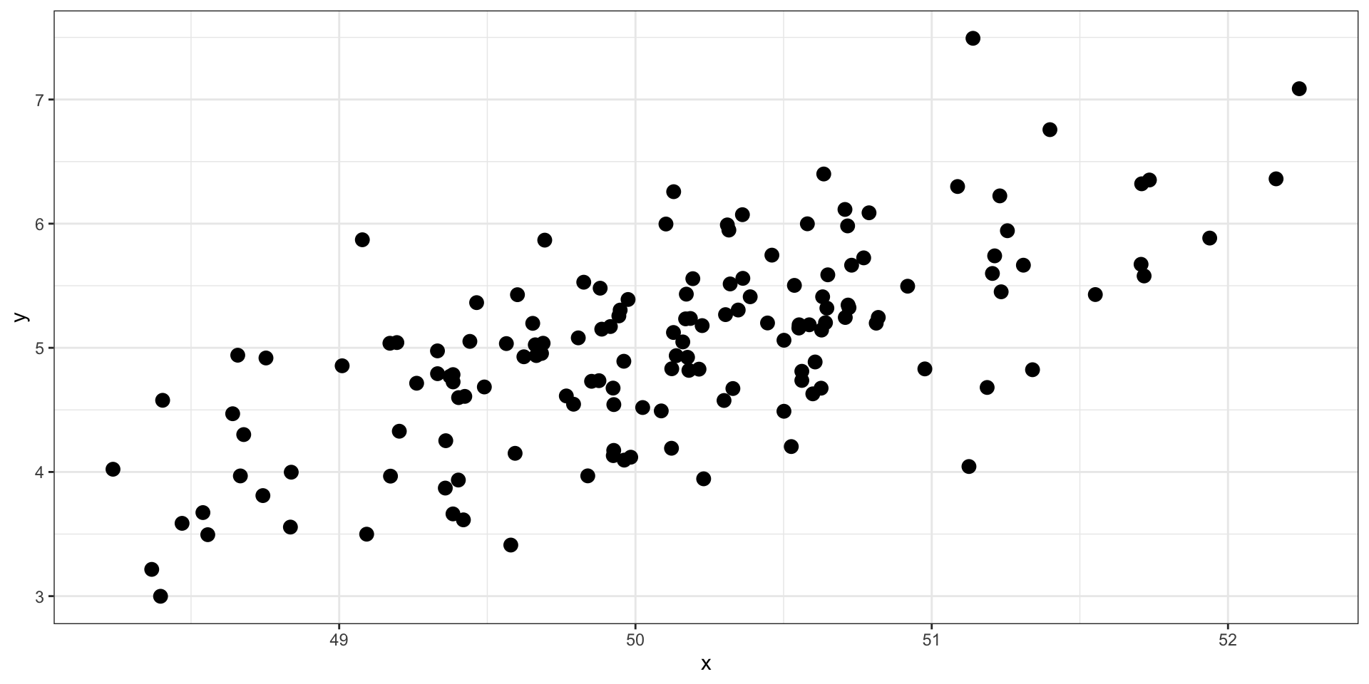
What is the correlation between these two variables?
Code
set.seed(101019) # so we all get the same random numbers
mu = c(10, 100)
Sigma = matrix(c(.8, -.3, -.3, .7), ncol =2) #diagonals are reliabilites, off-diagonals are correlations
data = mvrnorm(n = 150, mu = mu, Sigma = Sigma)
data = as.data.frame(data)
colnames(data) = c("x", "y")

data %>% ggplot(aes(x = x, y = y)) + geom_point(size = 3) + theme_bw()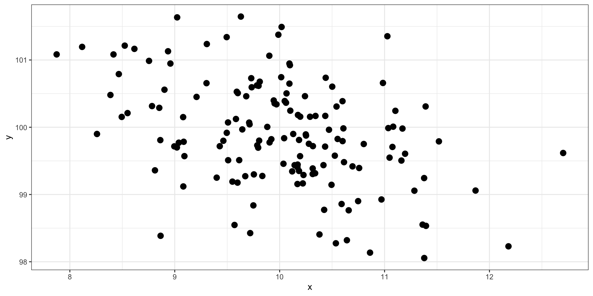
What is the correlation between these two variables?
Code
set.seed(101019) # so we all get the same random numbers
mu = c(3, 4)
Sigma = matrix(c(.8, 0, 0, .7), ncol =2) #diagonals are reliabilites, off-diagonals are correlations
data = mvrnorm(n = 150, mu = mu, Sigma = Sigma)
data = as.data.frame(data)
colnames(data) = c("x", "y")
data %>% ggplot(aes(x = x, y = y)) + geom_point(size = 3) + theme_bw()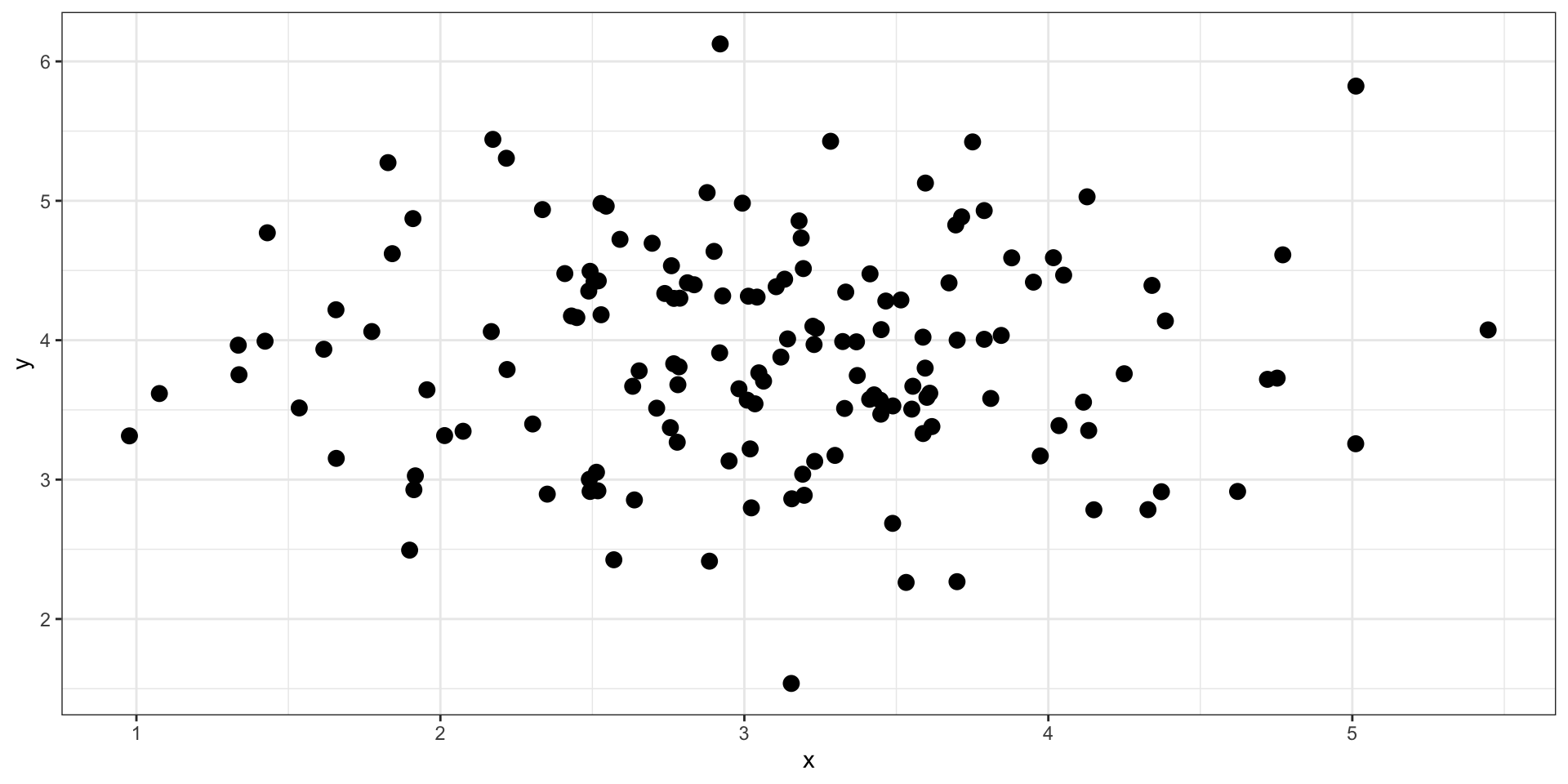
What is the correlation between these two variables?
Effect size
Recall that z-scores allow us to compare across units of measure; the products of standardized scores are themselves standardized.
The correlation coefficient is a standardized effect size which can be used communicate the strength of a relationship.
Correlations can be compared across studies, measures, constructs, time.
Example: the correlation between age and height among children is \(r = .70\). The correlation between self- and other-ratings of extraversion is \(r = .25\).
What is a large correlation?
- Cohen (1988): .1 (small), .3 (medium), .5 (large)
Often forgot: Cohen said only to use them when you had nothing else to go on, and has since regretted even suggesting benchmarks to begin with. |
Rosenthal & Rubin (1982): life and death (the Binomial Effect Size Display)
- treatment success rate \(= .50 + .5(r)\) and the control success rate \(= .50 - .5(r)\).
What is a large correlation?
- \(r^2\): Proportion of variance “explained”
- Ozer & Funder (2019) claim this is misleading and nonsensical
- Fisher (2019) suggests this particular argument is non-scientific (follow up here and then here)
Funder & Ozer (2019)
Effect sizes are often mis-interpreted. How?
What can fix this?
Pitfalls of small effects and large effects
Recommendations?
What affects correlations?
It’s not enough to calculate a correlation between two variables. You should always look at a figure of the data to make sure the number accurately describes the relationship. Correlations can be easily fooled by qualities of your data, like:
Skewed distributions
Outliers
Restriction of range
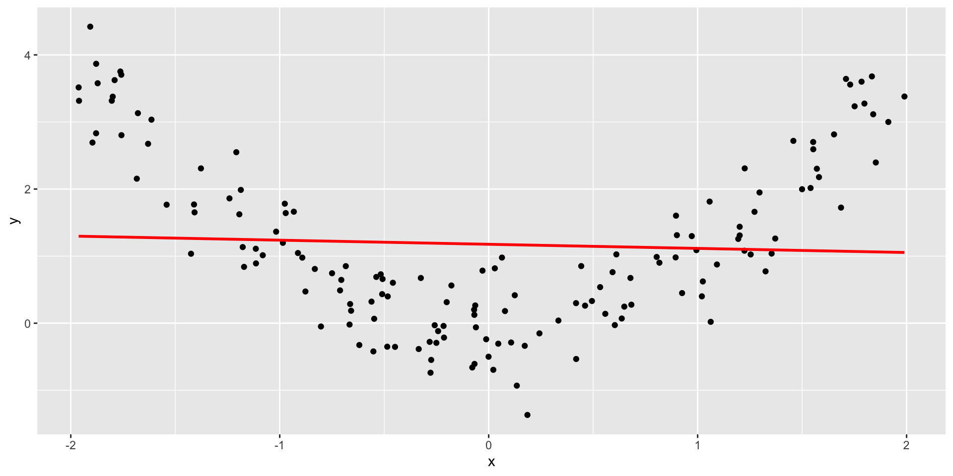
Nonlinearity
Skewed distributions
Code
set.seed(101019) # so we all get the same random numbers
mu = c(3, 4)
Sigma = matrix(c(.8, .2, .2, .7), ncol =2) #diagonals are reliabilites, off-diagonals are correlations
data = mvrnorm(n = 150, mu = mu, Sigma = Sigma)
data = as.data.frame(data)
colnames(data) = c("x", "y")
data$x = data$x^4

p = data %>% ggplot(aes(x=x, y=y)) + geom_point()
ggMarginal(p, type = "density")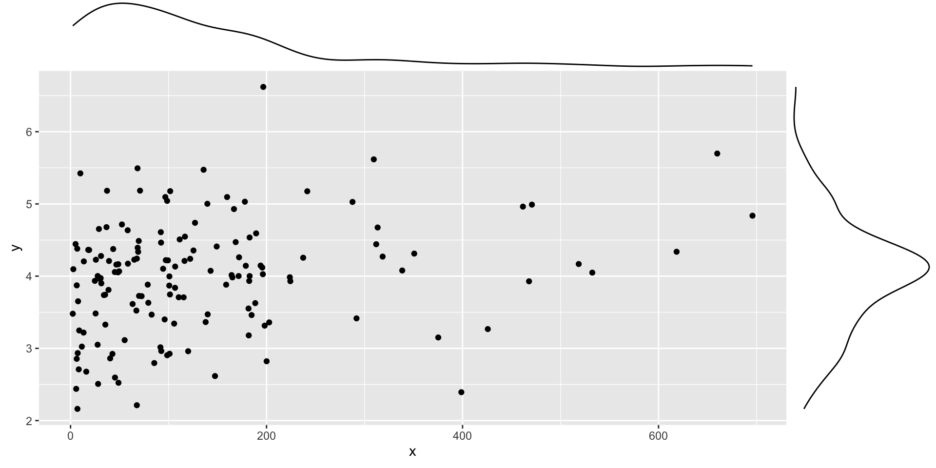
Outliers
Code
set.seed(101019) # so we all get the same random numbers
mu = c(3, 4)
Sigma = matrix(c(.8, 0, 0, .7), ncol =2) #diagonals are reliabilites, off-diagonals are correlations
data = mvrnorm(n = 50, mu = mu, Sigma = Sigma)
data = as.data.frame(data)
colnames(data) = c("x", "y")
data[51, ] = c(7, 10)
data %>% ggplot(aes(x=x, y=y)) + geom_point() 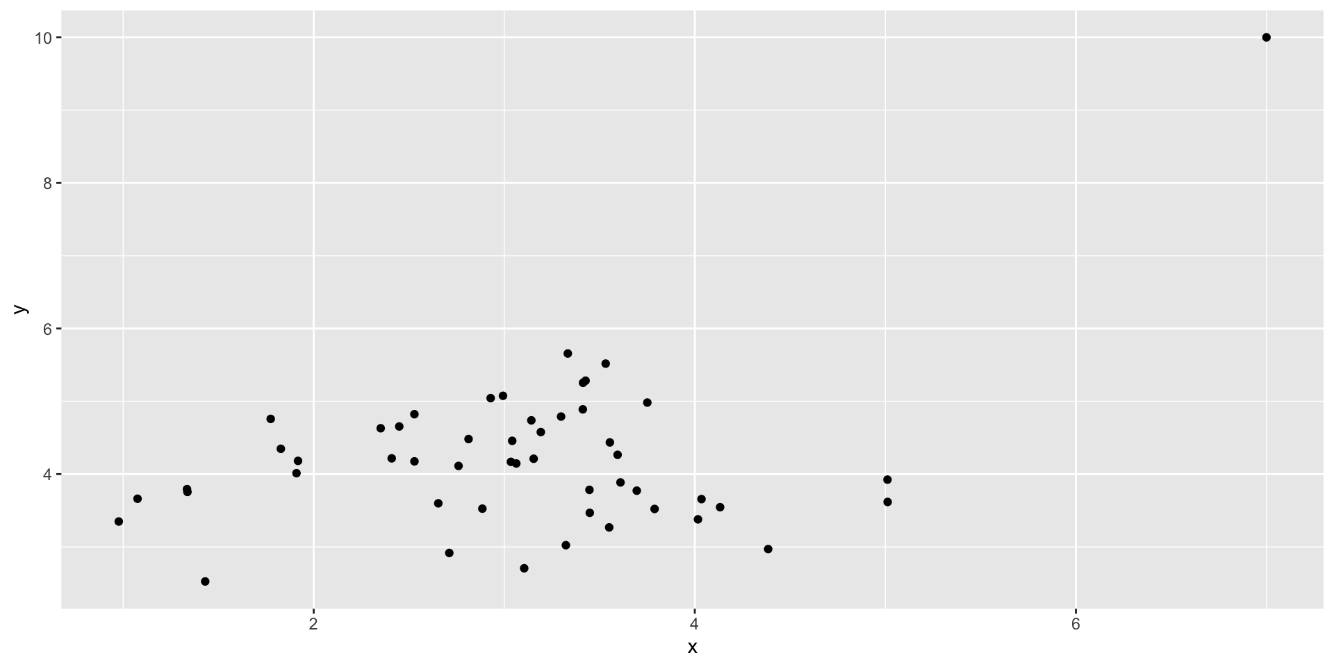
Outliers
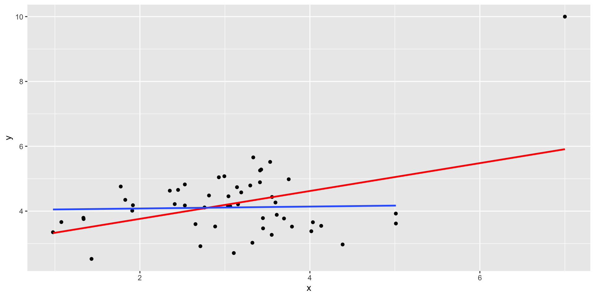
Outliers
Code
set.seed(101019) # so we all get the same random numbers
mu = c(3, 4)
n = 15
Sigma = matrix(c(.9, .8, .8, .9), ncol =2) #diagonals are reliabilites, off-diagonals are correlations
data = mvrnorm(n = n, mu = mu, Sigma = Sigma)
data = as.data.frame(data)
colnames(data) = c("x", "y")
data[n+1, ] = c(1.5, 5.5)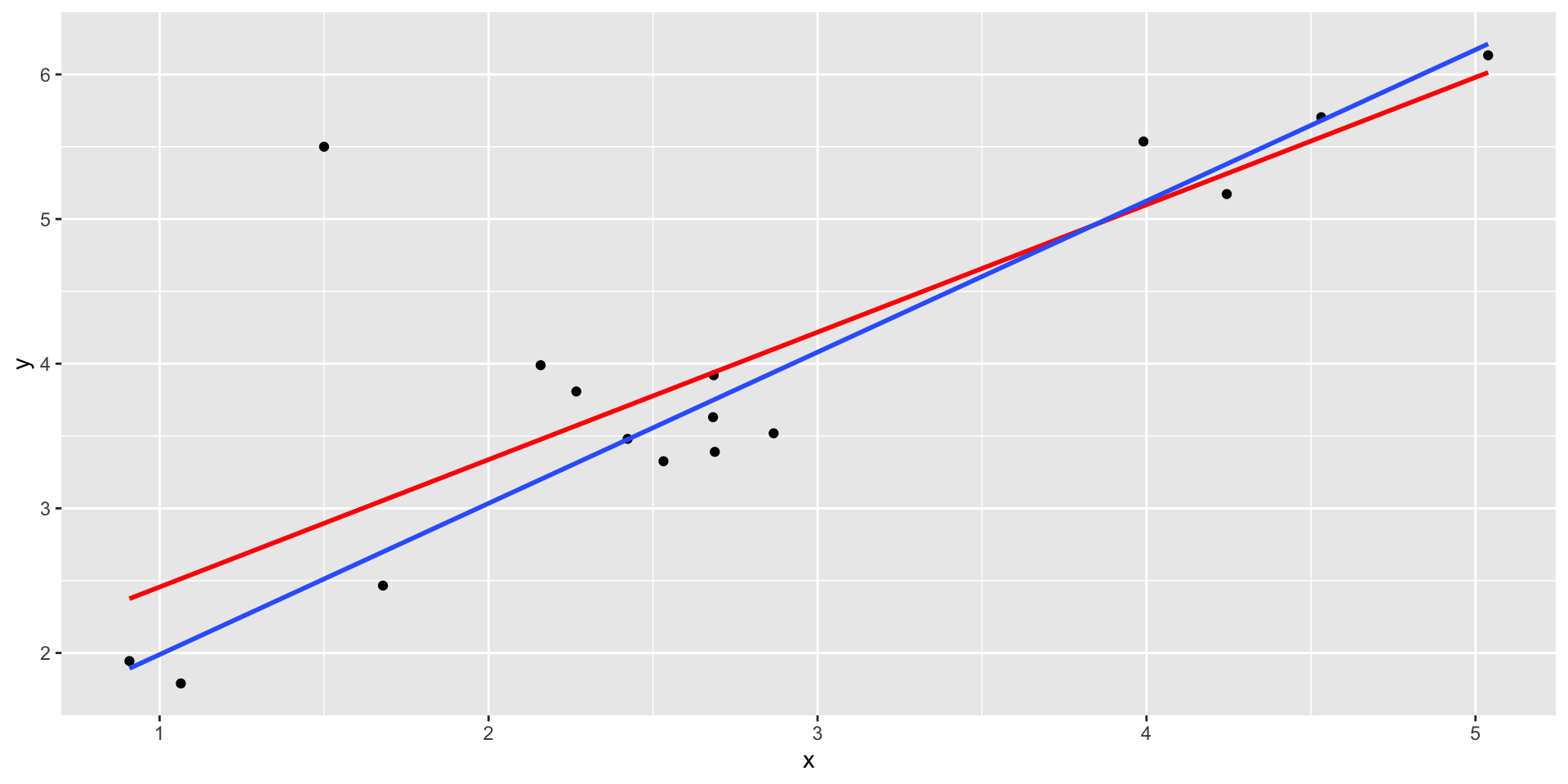
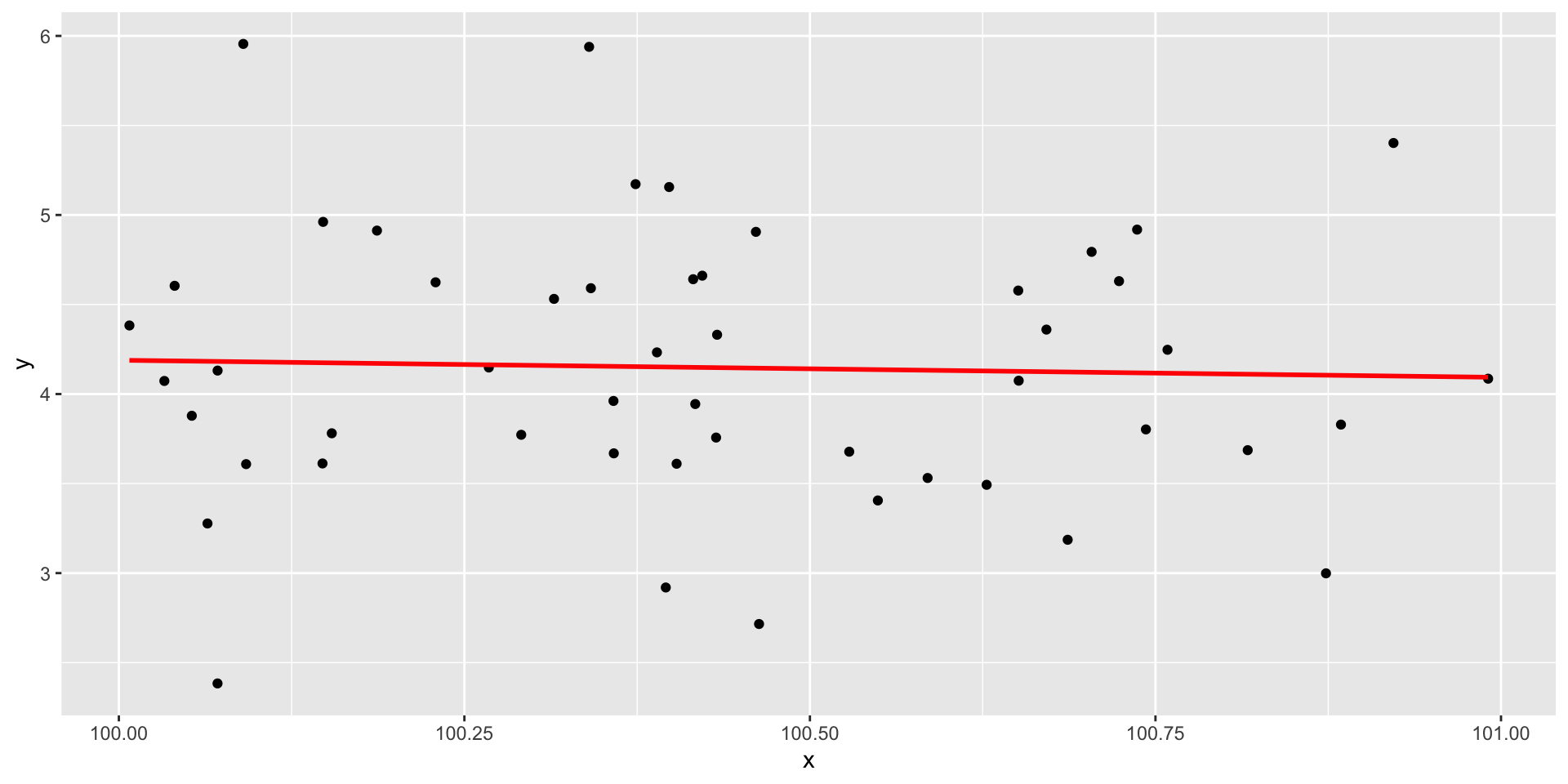
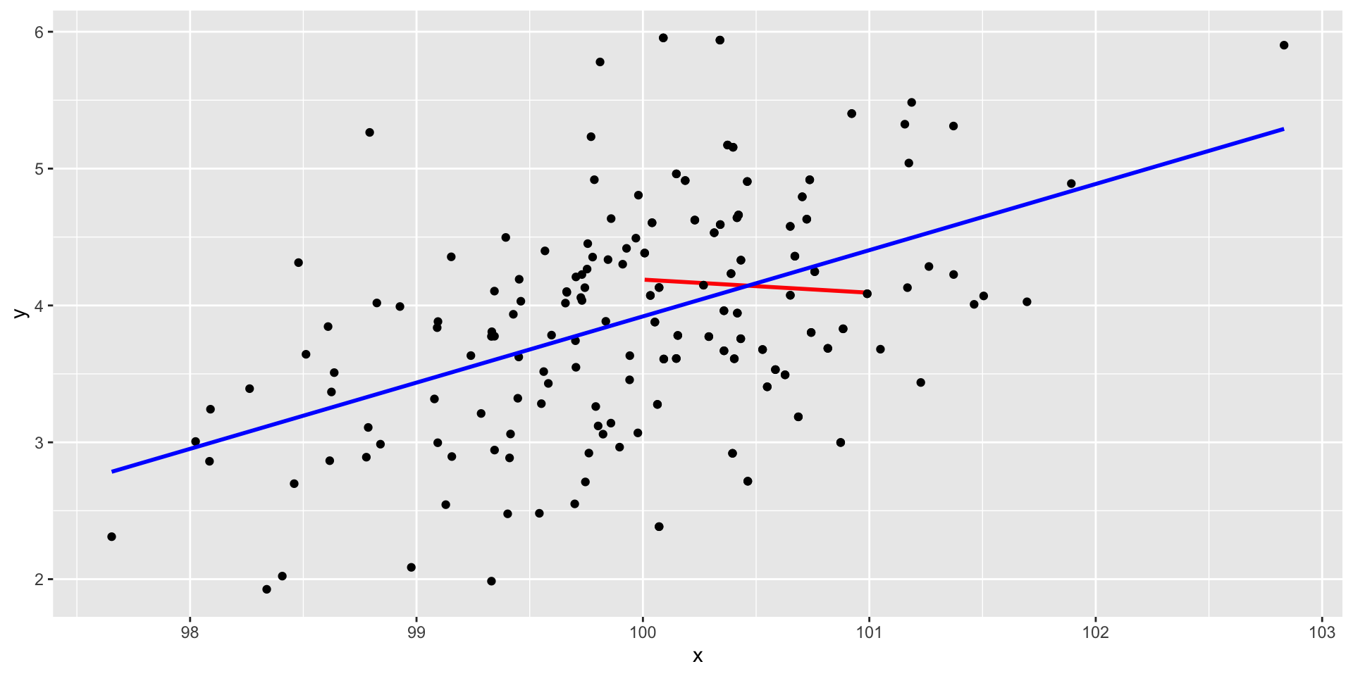
Restriction of range
Code
set.seed(1010191) # so we all get the same random numbers
mu = c(100, 4)
Sigma = matrix(c(.7, .4, 4, .75), ncol = 2) #diagonals are reliabilites, off-diagonals are correlations
data = mvrnorm(n = 150, mu = mu, Sigma = Sigma)
data = as.data.frame(data)
colnames(data) = c("x", "y")
real_data = data
data = filter(data, x >100 & x < 101)Restriction of range
Nonlinearity
It’s not always apparent
Sometimes issues that affect correlations won’t appear in your graph, but you still need to know how to look for them.
Low reliability
Content overlap
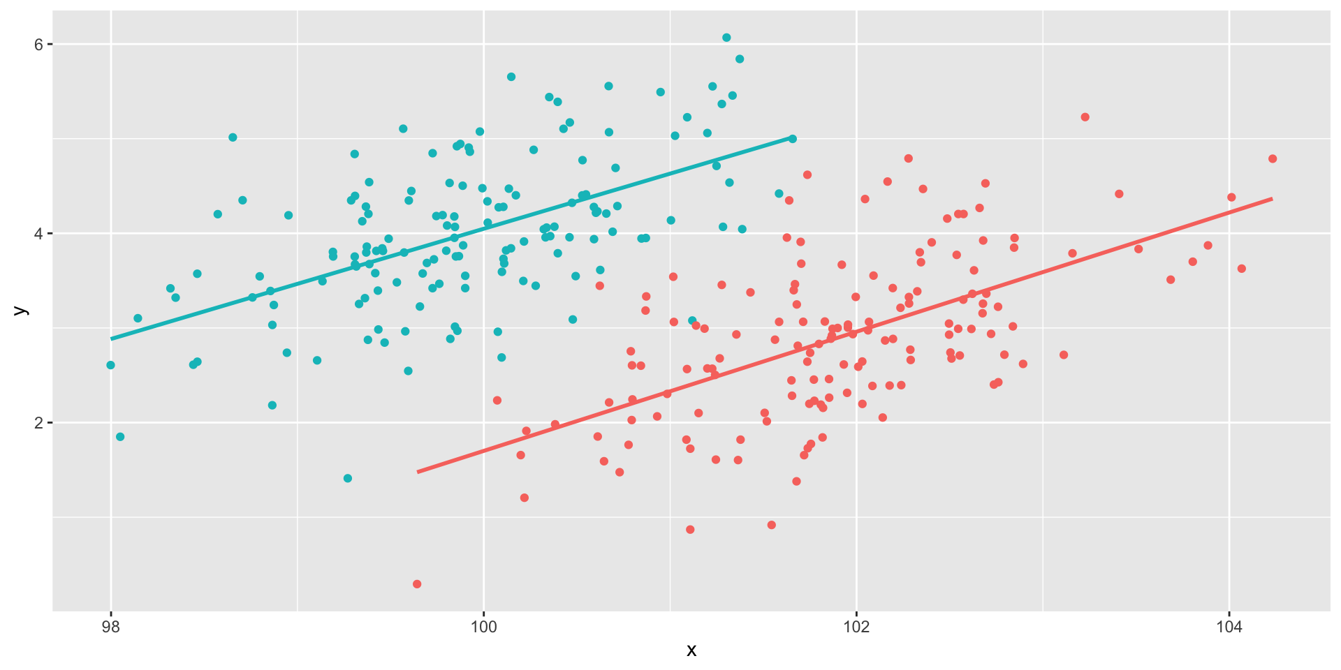
Multiple groups
Reliability
\[r_{xy} = \rho_{xy}\sqrt{r_{xx}r_{yy}}\]
Meaning that our estimate of the population correlation coefficient is attenuated in proportion to reduction in reliability.
If you have a bad measure of X or Y, you should expect a lower estimate of \(\rho\).
Content overlap
If your Operation Y of Construct B includes items (or tasks or manipulations) that could also be influenced by Constrct A, then the correlation between X and Y will be inflated.
Example: SAT scores and IQ tests
Example: Depression and number of hours sleeping
Which kind of validity is this associated with?
In-class demo
Add your height (in inches), forearm length (in inches), and gender to this spreadsheet: tinyurl.com/uwn463vj
Multiple groups
Code
set.seed(101019) # so we all get the same random numbers
m_mu = c(100, 4)
m_Sigma = matrix(c(.7, .4, 4, .75), ncol = 2) #diagonals are reliabilites, off-diagonals are correlations
m_data = mvrnorm(n = 150, mu = m_mu, Sigma = m_Sigma)
m_data = as.data.frame(m_data)
colnames(m_data) = c("x", "y")

f_mu = c(102, 3)
f_Sigma = matrix(c(.7, .4, 4, .75), ncol = 2) #diagonals are reliabilites, off-diagonals are correlations
f_data = mvrnorm(n = 150, mu = f_mu, Sigma = f_Sigma)
f_data = as.data.frame(f_data)
colnames(f_data) = c("x", "y")

m_data$gender = "male"
f_data$gender = "female"

data = rbind(m_data, f_data)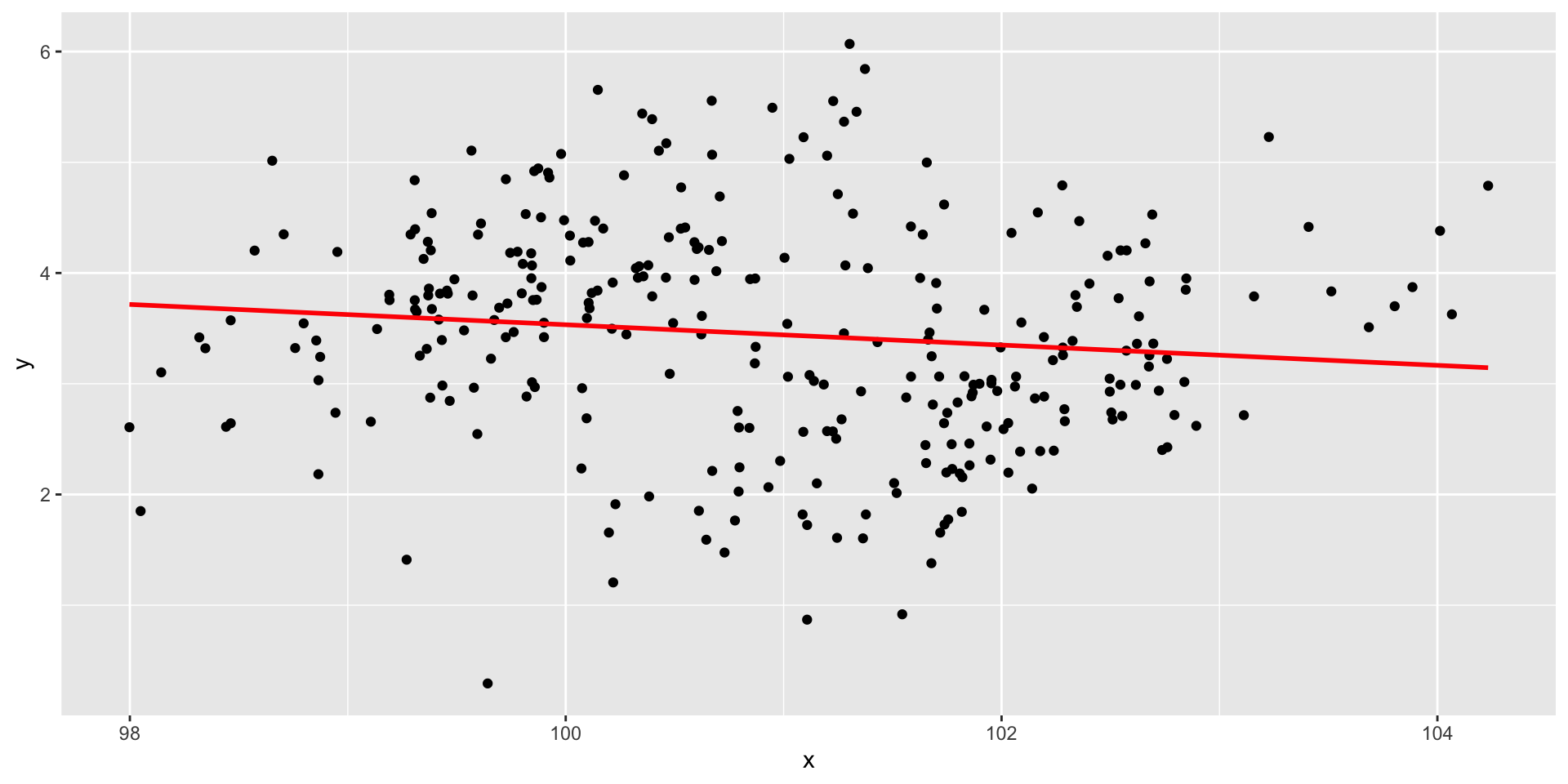
Multiple groups
Special cases of the Pearson correlation
- Spearman correlation coefficient
- Applies when both X and Y are ranks (ordinal data) instead of continuous
- Denoted \(\rho\) by your textbook, although I prefer to save Greek letters for population parameters.
- Point-biserial correlation coefficient
- Applies when Y is binary.
- Phi ( \(\phi\) ) coefficient
- Both X and Y are dichotomous.
Do the special cases matter?
For Spearman, you’ll get a different answer.
Here are two ways to analyze these data
Do the special cases matter?
If your data are naturally binary, no difference between Pearson and point-biserial.
               x y
[1,] -0.48974849 1
[2,] -2.53667101 0
[3,]  0.03521883 1
[4,]  0.03043436 0
[5,] -0.27043857 0
[6,] -0.55228283 1
Here are two ways to analyze these data
Do the special cases matter?
If artificially dichotomize data, there can be big differences. This is bad.
Here are two ways to analyze these data
Don’t use median splits!
Special cases of the Pearson correlation
Why do we have special cases of the correlation?
Sometimes we get different results
- If we treat ordinal data like interval/ratio data, our estimate will be incorrect
Sometimes we get the same result
Even when formulas are different
Example: Point biserial formula
- \[r_{pb} = \frac{M_1-M_0}{\sqrt{\frac{1}{n-1}\Sigma(X_i-\bar{X})^2}}\sqrt{\frac{n_1n_0}{n(n-1)}}\]
Next time…
Probability!
