Psy 612: Data Analysis II
Welcome back!
Last term:
- Descriptive statistics
- Probability
- Sampling
- Hypothesis testing
This term:
- Model building
- Correlation and regression
- General linear model
- Multiple regression
PSY 612 details
Structure of this course:
- Lectures, Labs, Reading
- Weekly quizzes (T/F)
- Homework assignments (3, 30 points each)
- Final project (1)
Journals are optional (no impact on grade)
PSY 612 goals
Understand how models are built and estimated
Exposure to a broad range of ideas and tools
- Can’t learn everything in a year – exposure helps you when you need to learn something new
Practice practical skills
- Looking up code online
- Troubleshooting errors
- Using real data, dealing with real problems
- Asking for help
Relationships
What is the relationship between IV and DV?
Measuring relationships depend on type of measurement
You have primarily been working with categorical IVs
- t-tests
- chi-square
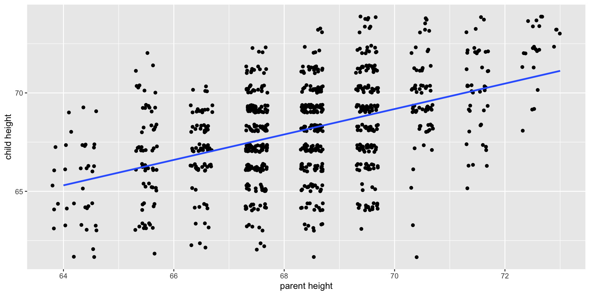
Scatter Plot with best fit line
Review of Dispersion
Variation (sum of squares)
\[SS = {\sum{(x-\bar{x})^2}}\] \[SS = {\sum{(x-\mu)^2}}\]
Review of Dispersion
Variance
\[\large s^{2} = \hat{\sigma}^2 = {\frac{\sum{(x-\bar{x})^2}}{N-1}}\]
\[\large\sigma^{2} = {\frac{\sum{(x-\mu)^2}}{N}}\]
Review of Dispersion
Standard Deviation
\[ s = \hat{\sigma} = \sqrt{\frac{\sum{(x-\bar{x})^2}}{N-1}}\]
\[\sigma = \sqrt{\frac{\sum{(x-\mu)^2}}{N}}\]
Formula for standard error of the mean?
\[\sigma_M = \frac{\sigma}{\sqrt{N}}\]
\[\sigma_M = \frac{s}{\sqrt{N}}\]
Associations
- i.e., relationships
- to look at continuous variable associations we need to think in terms of how variables relate to one another
Associations
Covariation (cross products)
Sample:
\[ SS = {\sum{(x-\bar{x})(y-\bar{y})}}\]
Population:
\[SS = {\sum{{(x-\mu_{x}})(y-\mu_{y})}}\]
Associations
Covariance
Sample:
\[ cov_{xy} = {\frac{\sum{(x-\bar{x})(y-\bar{y})}}{N-1}}\]
Population:
\[ \sigma_{xy}^{2} = {\frac{\sum{(x-\mu_{x})(y-\mu_{y})}}{N}}\]
- Covariance matrix is basis for many analyses
- What are some issues that may arise when comparing covariances?
Associations
Correlations
Sample:
\[ r_{xy} = {\frac{\sum({z_{x}z_{y})}}{N}}\]
Population:
\[\rho_{xy} = {\frac{cov(X,Y)}{\sigma_{x}\sigma_{y}}}\]
Many other formulas exist for specific types of data, these were more helpful when we computed everything by hand (more on this later).
Correlations
How much two variables are linearly related
-1 to 1
Invariant to changes in mean or scaling
Most common (and basic) effect size measure
Will use to build our regression model
Correlations
Conceptually
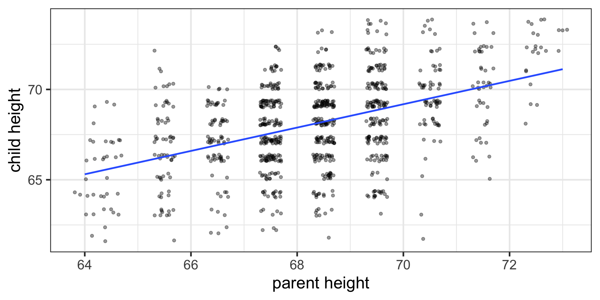
Ways to think about a correlation:
How two vectors of numbers co-relate
Product of z-scores
- Mathematically, it is
The average squared distance between two vectors in the same space
The cosine of the angle between Y and the projected Y from X \((\hat{Y})\).
Statistical test
Hypothesis testing
\[ H_{0}: \rho_{xy} = 0\]
\[ H_{A}: \rho_{xy} \neq 0\]
Assumes:
- Observations are independent
- Symmetric bivariate distribution (joint probability distribution)
Univariate distributions
Code
pop = ggplot(data.frame(x = seq(-30, 30)), aes(x)) +
  stat_function(fun = function(x) dnorm(x, m = 0, sd = 10),
                geom = "area", fill = purples[3]) +
  scale_x_continuous("X") +
  scale_y_continuous("density", labels = NULL) +
  ggtitle("Population")+
  theme_bw(base_size = 20)
sample = data.frame(x = rnorm(n = 30, m = 0, sd = 10)) %>%
  ggplot(aes(x = x)) +
  geom_histogram(fill = purples[2], color = "black", bins = 20) +
  scale_x_continuous("X", limits = c(-30, 30)) +
  scale_y_continuous("frequency", labels = NULL) +
  ggtitle("Sample")+
  theme_bw(base_size = 20)
sampling = ggplot(data.frame(x = seq(-30, 30)), aes(x)) +
  stat_function(fun = function(x) dnorm(x, m = 0, sd = 10/sqrt(30)),
                geom = "area", fill = purples[3]) +
  scale_x_continuous("X") +
  scale_y_continuous("density", labels = NULL) +
  ggtitle("Sampling")+
  theme_bw(base_size = 20)

ggpubr::ggarrange(pop, sample, sampling)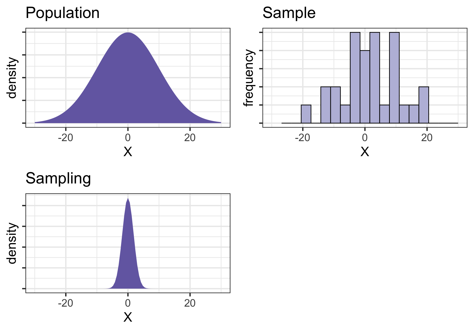
Population
Code
mu1<-0 # setting the expected value of x1
mu2<-0 # setting the expected value of x2
s11<-4 # setting the variance of x1
s12<-2 # setting the covariance between x1 and x2
s22<-5 # setting the variance of x2
rho<-0.1 # setting the correlation coefficient between x1 and x2
x1<-seq(-10,10,length=41) # generating the vector series x1
x2<-x1 # copying x1 to x2
f<-function(x1,x2){
    term1<-1/(2*pi*sqrt(s11*s22*(1-rho^2)))
    term2<--1/(2*(1-rho^2))
    term3<-(x1-mu1)^2/s11
    term4<-(x2-mu2)^2/s22
    term5<--2*rho*((x1-mu1)*(x2-mu2))/(sqrt(s11)*sqrt(s22))
    term1*exp(term2*(term3+term4-term5))
} # setting up the function of the multivariate normal density
#
z<-outer(x1,x2,f) # calculating the density values
#
persp(x1, x2, z,
main="Joint Probability Distribution", sub=expression(italic(f)~(bold(x))==frac(1,2~pi~sqrt(sigma[11]~ sigma[22]~(1-rho^2)))~phantom(0)^bold(.)~exp~bgroup("{", list(-frac(1,2(1-rho^2)),
bgroup("[", frac((x[1]~-~mu[1])^2, sigma[11])~-~2~rho~frac(x[1]~-~mu[1], sqrt(sigma[11]))~ frac(x[2]~-~mu[2],sqrt(sigma[22]))~+~ frac((x[2]~-~mu[2])^2, sigma[22]),"]")),"}")),
col= purples[3],
theta=30, phi=20,
r=50,
d=0.1,
expand=0.5,
ltheta=90, lphi=180,
shade=0.75,
ticktype="detailed",
nticks=5)

# produces the 3-D plot
mtext(expression(list(mu[1]==0,mu[2]==0,sigma[11]==4,sigma[22]==5,sigma[12 ]==2,rho==0.1)), side=3)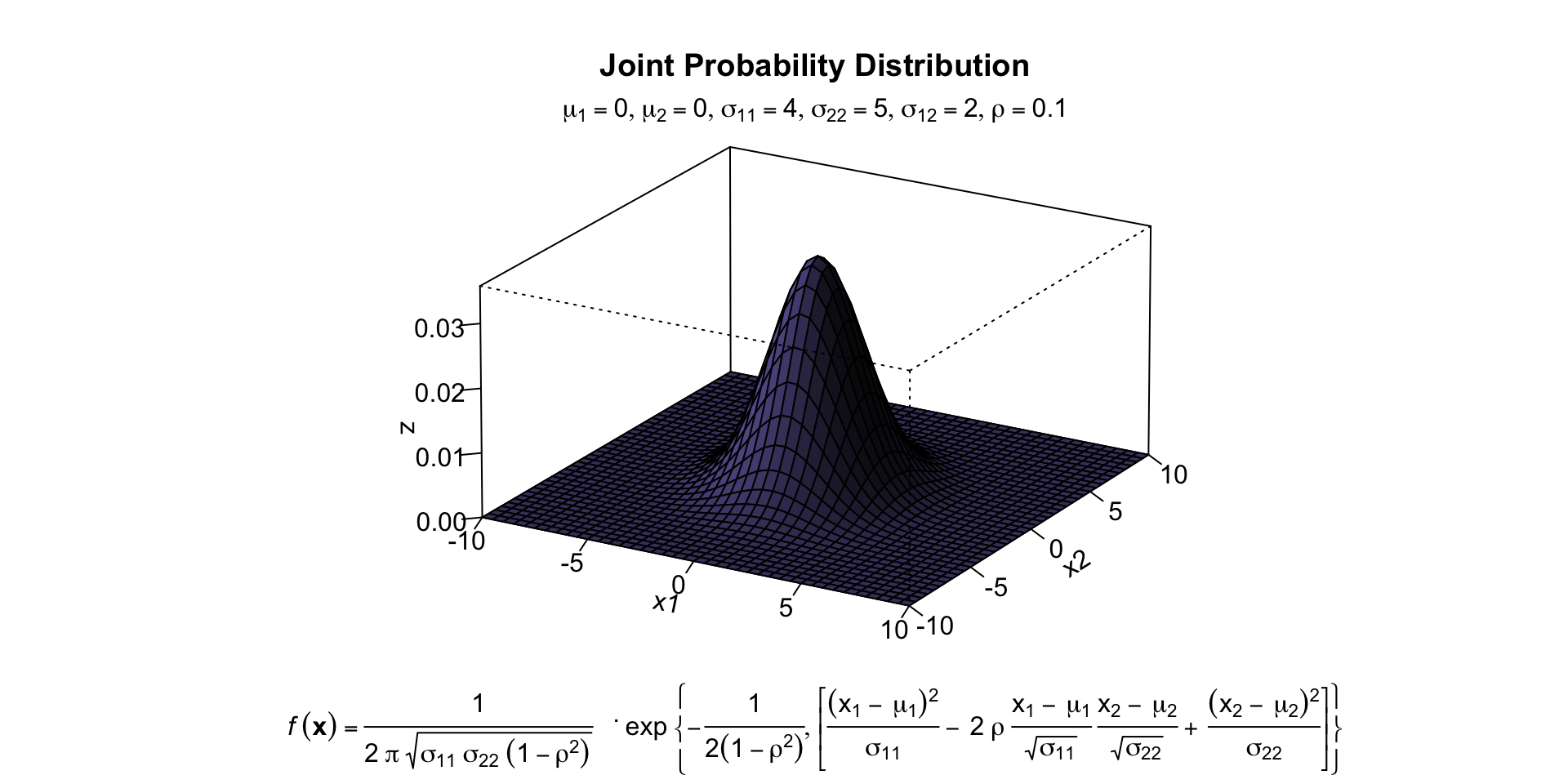
Sample
Code
sigma <- matrix( c( 4, 2,
                    2, 5 ), 2, 2 )  # covariance matrix

sample = BDgraph::rmvnorm(n = 30, mean = c(0,0), sigma = sigma)

sample %>% as.data.frame() %>%
  ggplot(aes(x = V1, y = V2)) +
  geom_smooth(method = "lm", se = F, color = purples[2])+
  geom_point(color = purples[3]) +
  scale_x_continuous("X1") +
  scale_y_continuous("X2")+
  theme_bw(base_size = 20)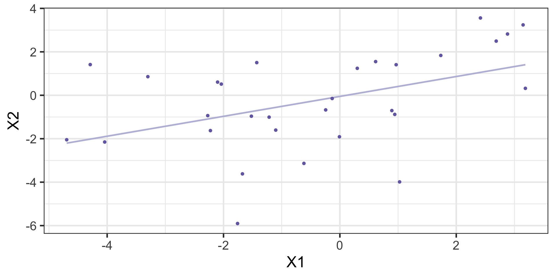
Sampling distribution?
The sampling distribution we use depends on our null hypothesis.
If our null hypothesis is the nil \((\rho = 0)\) , then we can use a t-distribution to estimate the statistical significance of a correlation.
Statistical test
Test statistic
\[\large t = {\frac{r}{SE_{r}}}\]
\[SE_r = \sqrt{\frac{1-r^2}{N-2}}\]
\[t = {\frac{r}{\sqrt{\frac{1-r^{2}}{N-2}}}}\]
\[ DF = N-2\]
Example
You’re comparing scores on the GRE Quantitative section and GRE Verbal section. You randomly select 30 applications out of those submitted to the University of Oregon and find a correlation between these scores of .80. Is this significantly different from 0?
Power calculations
     approximate correlation power calculation (arctangh transformation)

              n = 781.7516
              r = 0.1
      sig.level = 0.05
          power = 0.8
    alternative = two.sided
     approximate correlation power calculation (arctangh transformation)

              n = 84.07364
              r = 0.3
      sig.level = 0.05
          power = 0.8
    alternative = two.sided
Confidence intervals
But here’s where we get into some trouble. What happens if we try to estimate the precision around our estimate using the techniques we learned in PSY 611?
For the CI around a mean or a difference in means, we would use: \[CI_{95} = \bar{X} \pm SE(t_{\text{critical value}})\]
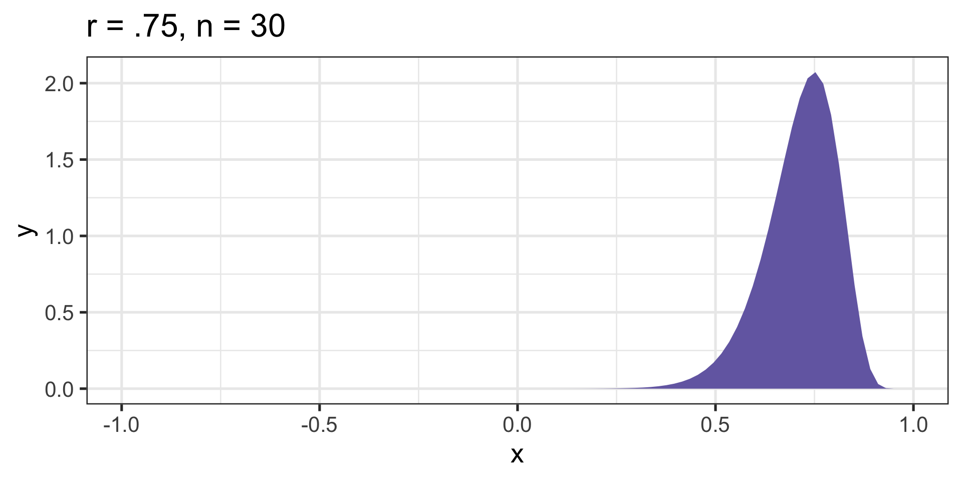
Sampling distributions are skewed
If we want to make calculations around correlation values that are not equal to 0, then we will run into a skewed sampling distribution. This applies to both calculating confidence intervals around estimates of correlations and null hypotheses in which \(\rho \neq 0\).
Skewed sampling distributions
Code
r_sampling = function(x, r, n){
  z = fisherz(r)
  se = 1/(sqrt(n-3))
  x_z = fisherz(x)
  density = dnorm(x_z, mean = z, sd = se)
  return(density)
}

cor_75 = ggplot(data.frame(x = seq(-.99, .99)), aes(x)) +
  stat_function(fun = function(x) r_sampling(x, r = .75,
                                             n = 30),
                geom = "area", fill = purples[3]) +
  scale_x_continuous(limits = c(-.99, .99)) +
  ggtitle("r = .75, n = 30") +
  theme_bw(base_size = 20)

cor_32 = ggplot(data.frame(x = seq(-.99, .99)), aes(x)) +
  stat_function(fun = function(x) r_sampling(x, r = .32,
                                             n = 30),
                geom = "area", fill = purples[2]) +
  scale_x_continuous(limits = c(-.99, .99)) +
  ggtitle("r = .32, n = 30")+
  theme_bw(base_size = 20)


cor_n85 = ggplot(data.frame(x = seq(-.99, .99)), aes(x)) +
  stat_function(fun = function(x) r_sampling(x, r = -.85,
                                             n = 30),
                geom = "area", fill = purples[3]) +
  scale_x_continuous(limits = c(-.99, .99)) +
  ggtitle("r = -.85, n = 30")+
  theme_bw(base_size = 20)

cor_75b = ggplot(data.frame(x = seq(-.99, .99)), aes(x)) +
  stat_function(fun = function(x) r_sampling(x, r = .75,
                                             n = 150),
                geom = "area", fill = purples[3]) +
  scale_x_continuous(limits = c(-.99, .99)) +
  ggtitle("r = .75, n = 150") +
  theme_bw(base_size = 20)

cor_32b = ggplot(data.frame(x = seq(-.99, .99)), aes(x)) +
  stat_function(fun = function(x) r_sampling(x, r = .32,
                                             n = 150),
                geom = "area", fill = purples[2]) +
  scale_x_continuous(limits = c(-.99, .99)) +
  ggtitle("r = .32, n = 150")+
  theme_bw(base_size = 20)


cor_n85b = ggplot(data.frame(x = seq(-.99, .99)), aes(x)) +
  stat_function(fun = function(x) r_sampling(x, r = -.85,
                                             n = 150),
                geom = "area", fill = purples[3]) +
  scale_x_continuous(limits = c(-.99, .99)) +
  ggtitle("r = -.85, n = 150")+
  theme_bw(base_size = 20)


ggpubr::ggarrange(cor_n85, cor_32, cor_75,
                  cor_n85b, cor_32b, cor_75b)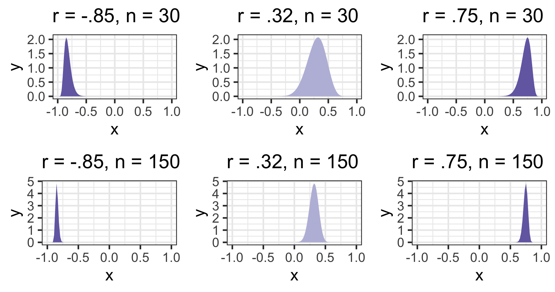
Skewed sampling distribution will rear their heads when:
\(H_{0}: \rho \neq 0\)
Calculating confidence intervals
Testing two correlations against one another
Fisher’s r to z’ transformation
- r to z’:
\[ z^{'} = {\frac{1}{2}}ln{\frac{1+r}{1-r}}\]
Fisher’s r to z’ transformation
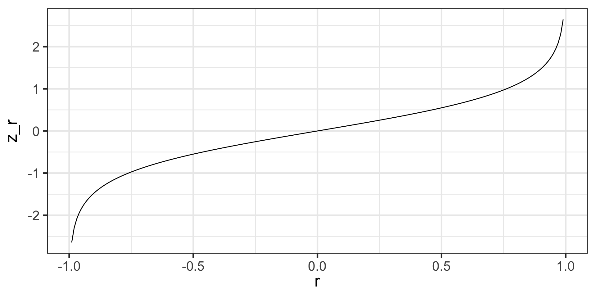
Steps for computing confidence interval
- Transform r into z’ 1
- Compute CI as you normally would using z’
- Reconvert back to r
\[ SE_z = \frac{1}{\sqrt{N-3}}\]
\[r = {\frac{e^{2z'}-1}{e^{2z'}+1}}\]
Example
In a sample of 42 students, you calculate a correlation of 0.44 between hours spent outside on Saturday and self-rated health. What is the precision of your estimate?
\[z = {\frac{1}{2}}ln{\frac{1+.44}{1-.44}} = 0.47\] \[SE_z = \frac{1}{\sqrt{42-3}} = 0.16\]
\[CI_{Z_{LB}} = 0.47-(1.96)0.16 = 0.16\]
\[CI_{Z_{UB}} = 0.47+(1.96)0.16 = 0.79\]
\[CI_{r_{LB}} = {\frac{e^{2(0.16)}-1}{e^{2(0.16)}+1}} = 0.16\]
\[CI_{r_{UB}} = {\frac{e^{2(0.79)}-1}{e^{2(0.79)}+1}} = 0.66\]
These formulas are easy to mistype in R – use the psych package and its functions fisherz() and fisherz2r() to save time and reduce human error.
Comparing two correlations
Again, we use the Fisher’s r to z’ transformation. Here, we’re transforming the correlations into z’s, then using the difference between z’s to calculate the test statistic.
\[Z = \frac{z_1^{'}- z_2^{'}}{se_{z_1-z_2}}\]
\[se_{z_1-z_2} = \sqrt{se_{z_1}+se_{z_2}} = \sqrt{\frac{1}{n_1-3}+\frac{1}{n_2-3}}\]
Example
You measure narcissism and happiness in two sets of adults: young adults (19-25) and older adults (over 25). You calculate the correlations separately for these two groups, and you want to know whether this relationship is stronger for one group or another.
Young adults
\[N = 327\] \[r = .402\]
Older adults
\[N = 273\] \[r = .283\]
\[H_0:\rho_1 = \rho_2\] \[H_1:\rho_1 \neq \rho_2\]
Effect size
The strength of relationship between two variables
\(\eta^2\), Cohen’s d, Cohen’s f, hedges g, \(R^2\) , Risk-ratio, etc
Significance is a function of effect size and sample size
Statistical significance \(\neq\) practical significance
Next time…
More correlations