Multiple regression

Part 1

Last time

• Semi-partial and partial correlations

Today

• Introduction to multiple regression

library(tidyverse)

Regression equation

\[\large \hat{Y} = b_0 + b_1X_1 + b_2X_2 + \dots+b_kX_k\] Regression coefficients are “partial” regression coefficients

• predicted change in \(Y\) for a 1 unit change in \(X\), holding all other predictors constant

• similar in interpretation to semi-partial correlation – represents contribution to all of Y from unique part of each \(X\)

• same statistical test as partial correlation – unique variance of \(Y\) explained by unique variance of each \(X\)

example

library(here); library(tidyverse)
support_df = read.csv(here("data/support.csv")) 
library(psych)
describe(support_df, fast = T)

                vars  n mean   sd  min  max range   se
give_support       1 78 4.99 1.07 2.77 7.43  4.66 0.12
receive_support    2 78 7.88 0.85 5.81 9.68  3.87 0.10
relationship       3 78 5.85 0.86 3.27 7.97  4.70 0.10

round(cor(support_df),2)

                give_support receive_support relationship
give_support            1.00            0.39         0.36
receive_support         0.39            1.00         0.45
relationship            0.36            0.45         1.00

example

mr.model <- lm(relationship ~ receive_support + give_support, data = support_df)
summary(mr.model)

...
Coefficients:
                Estimate Std. Error t value Pr(>|t|)   
(Intercept)      2.07212    0.81218   2.551  0.01277 * 
receive_support  0.37216    0.11078   3.359  0.00123 **
give_support     0.17063    0.08785   1.942  0.05586 . 
...

# partial correlation tests
with(support_df, ppcor::pcor.test(relationship, receive_support, give_support))

   estimate     p.value statistic  n gp  Method
1 0.3616442 0.001230843  3.359301 78  1 pearson

with(support_df, ppcor::pcor.test(relationship, give_support, receive_support))

  estimate    p.value statistic  n gp  Method
1 0.218838 0.05585914  1.942271 78  1 pearson

Note that significance of partial effects is identital.

If a univariate regression is estimating the best-fit line, what is this estimating?

Visualizing multiple regression

library(visreg)

visreg2d(mr.model,"receive_support", "give_support", plot.type = "persp")

Calculating coefficients

Just like with univariate regression, we calculate the OLS solution. As a reminder, this calculation will yield the estimate that reduces the sum of the squared deviations from the line:

Unstandardized

\[\large \hat{Y} = b_0 + b_{1}X1 + b_{2}X_2\] \[\large \text{minimize} \sum (Y-\hat{Y})^2 \]

Standardized

\[\large \hat{Z}_{Y} = b_{1}^*Z_{X1} + b_{2}^*Z_{X2}\] \[\large \text{minimize} \sum (z_{Y}-\hat{z}_{Y})^2\]

Calculating the standardized regression coefficient

\[b_{1}^* = \frac{r_{Y1}-r_{Y2}r_{12}}{1-r_{12}^2}\]

\[b_{2}^* = \frac{r_{Y2}-r_{Y1}r_{12}}{1-r_{12}^2}\]

Relationships between partial, semi- and \(b*\)

(Standardized) Regression coefficients, partial correlations, and semi-partial correlations are all ways to represent the relationship between two variables while taking into account a third (or more!) variables.

Each is a standardized effect, meaning the effect size is calculated in standardized units, bounded by -1 and 1¹. This means they can be compared across studies, metrics, etc.

1. Actually, standardized regression coefficients are not bounded by -1 and 1, but it’s rare to see values this large, and usually indicative of some multicollinearity.

Relationships between partial, semi- and \(b*\)

Note, however, that the calculations differ between the three effect sizes. These effect sizes are not synonymous and often yield different answers.

• if predictors are not correlated, \(r\), \(sr\) \((r_{Y(1.2)})\) and \(b*\) are equal

Standardized multiple regression coefficient, \(b^*\)

\[\large \frac{r_{Y1}-r_{Y2}r_{12}}{1-r_{12}^2}\]

Semi-partial correlation, \(r_{y(1.2)}\) \[\large \frac{r_{Y1}-r_{Y2}r_{Y12} }{\sqrt{1-r_{12}^2}}\]

Partial correlation, \(r_{y1.2}\) \[\large \frac{r_{Y1}-r_{Y2}r_{{12}}}{\sqrt{1-r^2_{Y2}}\sqrt{1-r^2_{12}}}\]

Regression coefficient is most similar to the semi-partial correlation coefficient.

See here how the estimates differ from one another:

support_df = support_df %>%
  mutate(z_give_support = scale(give_support),
         z_receive_support = scale(receive_support),
         z_relationship = scale(relationship))

mod0 = lm(z_relationship ~ z_give_support + z_receive_support, 
          data = support_df)

#extract partial slope for give support
round(coef(mod0)["z_give_support"],3)

z_give_support 
         0.212 

spcor.test(x = support_df$relationship, 
           y = support_df$give_support, 
           z = support_df$receive_support)$estimate

[1] 0.1953065

pcor.test(x = support_df$relationship, 
          y = support_df$give_support, 
          z = support_df$receive_support)$estimate

[1] 0.218838

Original metric

\[b_{1} = b_{1}^*\frac{s_{Y}}{s_{X1}}\]

\[b_{1}^* = b_{1}\frac{s_{X1}}{s_{Y}}\]

Intercept

\[b_{0} = \bar{Y} - b_{1}\bar{X_{1}} - b_{2}\bar{X_{2}}\]

mr.model <- lm(relationship ~ receive_support + give_support, data = support_df)
summary(mr.model)

...

Call:
lm(formula = relationship ~ receive_support + give_support, data = support_df)

Residuals:
     Min       1Q   Median       3Q      Max 
-2.26837 -0.40225  0.07701  0.42147  1.76074 

Coefficients:
                Estimate Std. Error t value Pr(>|t|)   
(Intercept)      2.07212    0.81218   2.551  0.01277 * 
...

Highlight intercept value: what does this mean?

mr.model <- lm(relationship ~ receive_support + give_support, data = support_df)
summary(mr.model)

...

Call:
lm(formula = relationship ~ receive_support + give_support, data = support_df)

Residuals:
     Min       1Q   Median       3Q      Max 
-2.26837 -0.40225  0.07701  0.42147  1.76074 

Coefficients:
                Estimate Std. Error t value Pr(>|t|)   
(Intercept)      2.07212    0.81218   2.551  0.01277 * 
receive_support  0.37216    0.11078   3.359  0.00123 **
give_support     0.17063    0.08785   1.942  0.05586 . 
...

Next, how to interpret those slope values?

“Controlling for”

“Controlling for”

Taken from @nickchk

Compare the slopes

un.model <- lm(relationship ~ give_support,           data = support_df)
summary(un.model)

...
Coefficients:
             Estimate Std. Error t value            Pr(>|t|)    
(Intercept)   4.42369    0.43882  10.081 0.00000000000000117 ***
give_support  0.28681    0.08605   3.333             0.00133 ** 
...

mr.model <- lm(relationship ~ receive_support + give_support, data = support_df)
summary(mr.model)

...
Coefficients:
                Estimate Std. Error t value Pr(>|t|)   
(Intercept)      2.07212    0.81218   2.551  0.01277 * 
receive_support  0.37216    0.11078   3.359  0.00123 **
give_support     0.17063    0.08785   1.942  0.05586 . 
...

library(sjPlot)
plot_model(un.model, type = "pred", terms = c("give_support")) + ylim(4.5, 7.5)

library(sjPlot)
plot_model(mr.model, type = "pred", terms = c("give_support")) + ylim(4.5, 7.5)

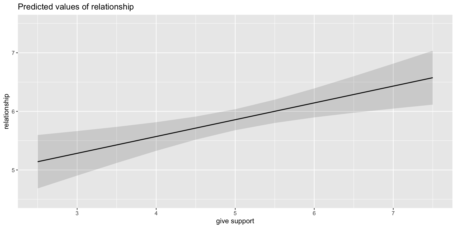
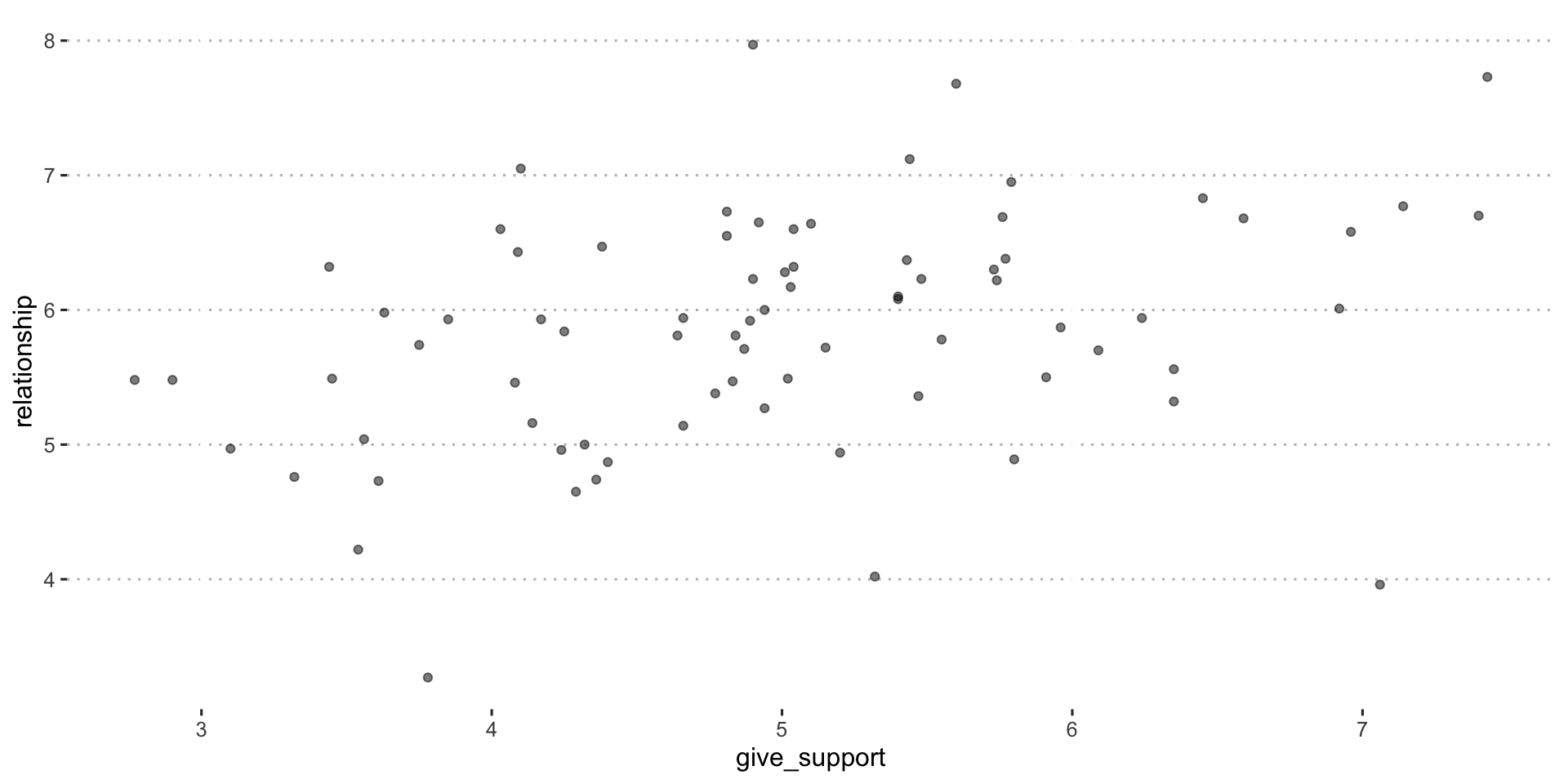
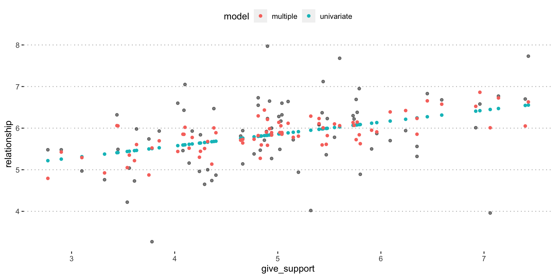
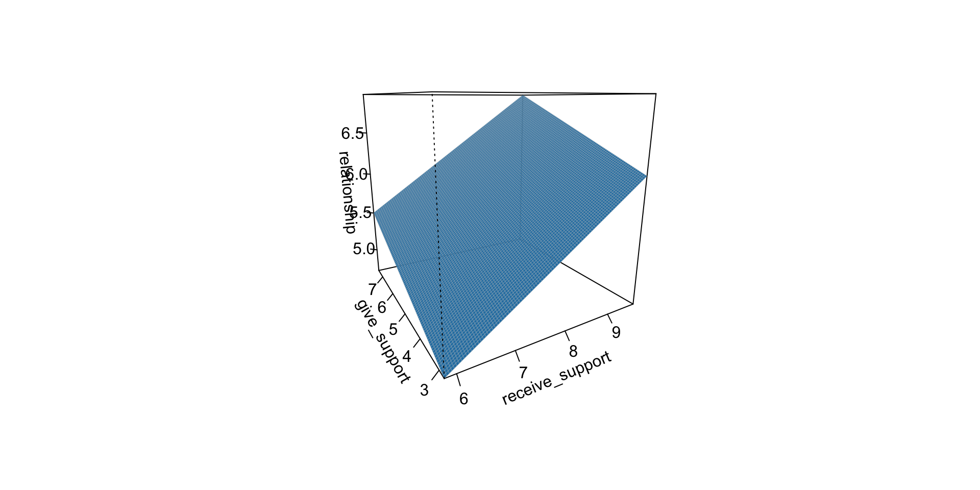
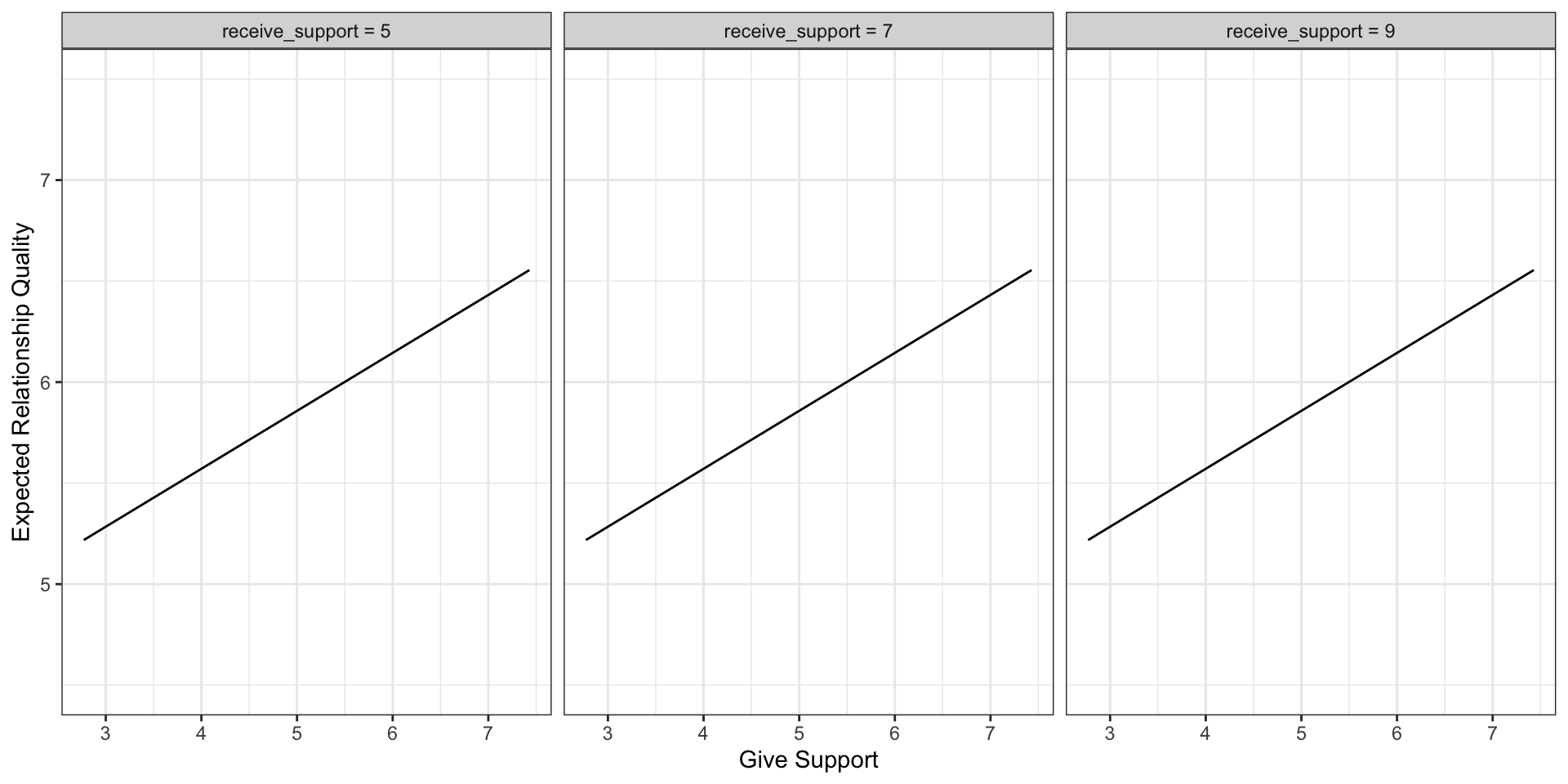
Predictions: univariate model

Predictions: multiple regression model

plot_model(mr.model, type = "pred", 
           terms = c("give_support", "receive_support[meansd]"))

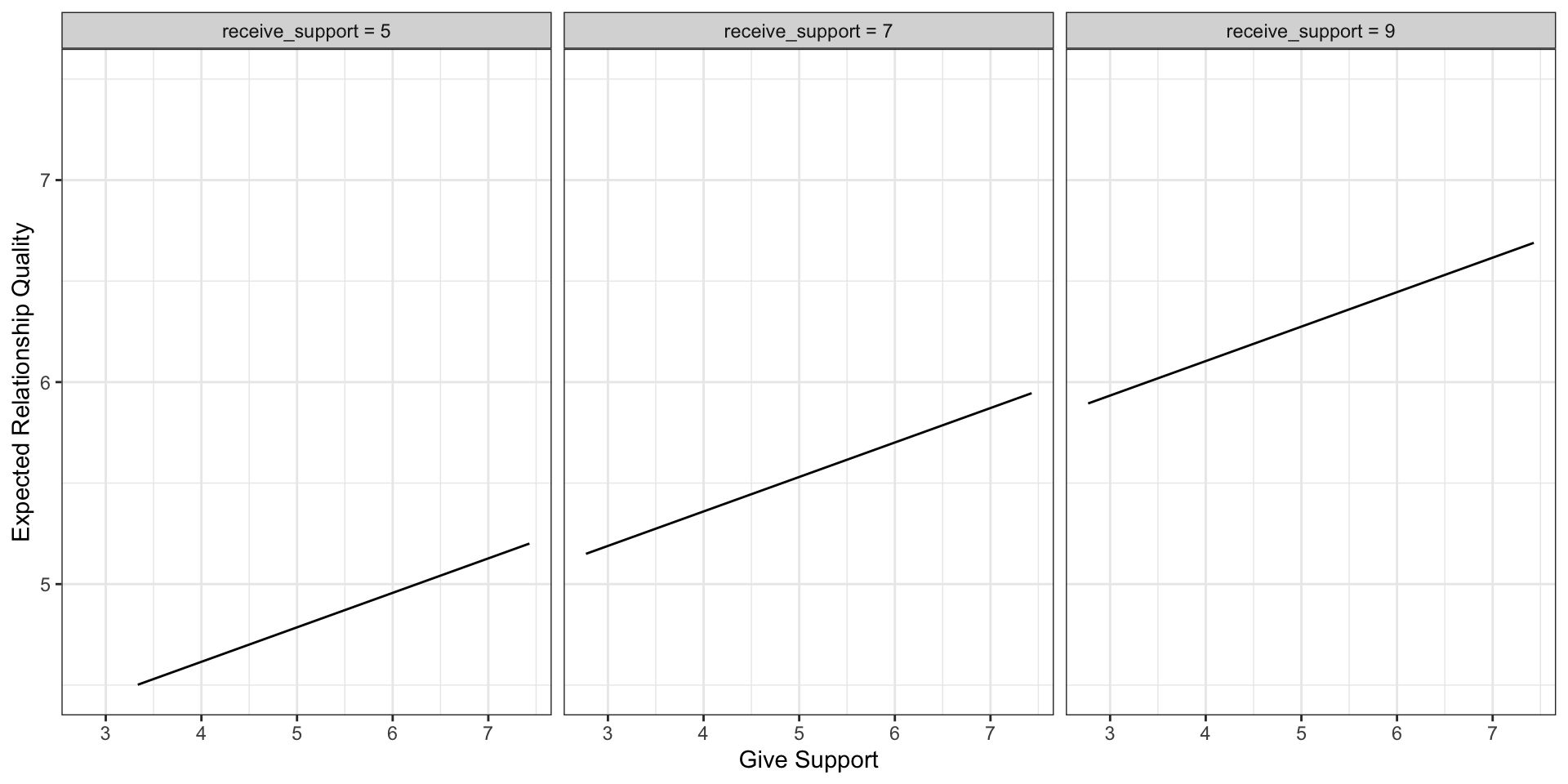
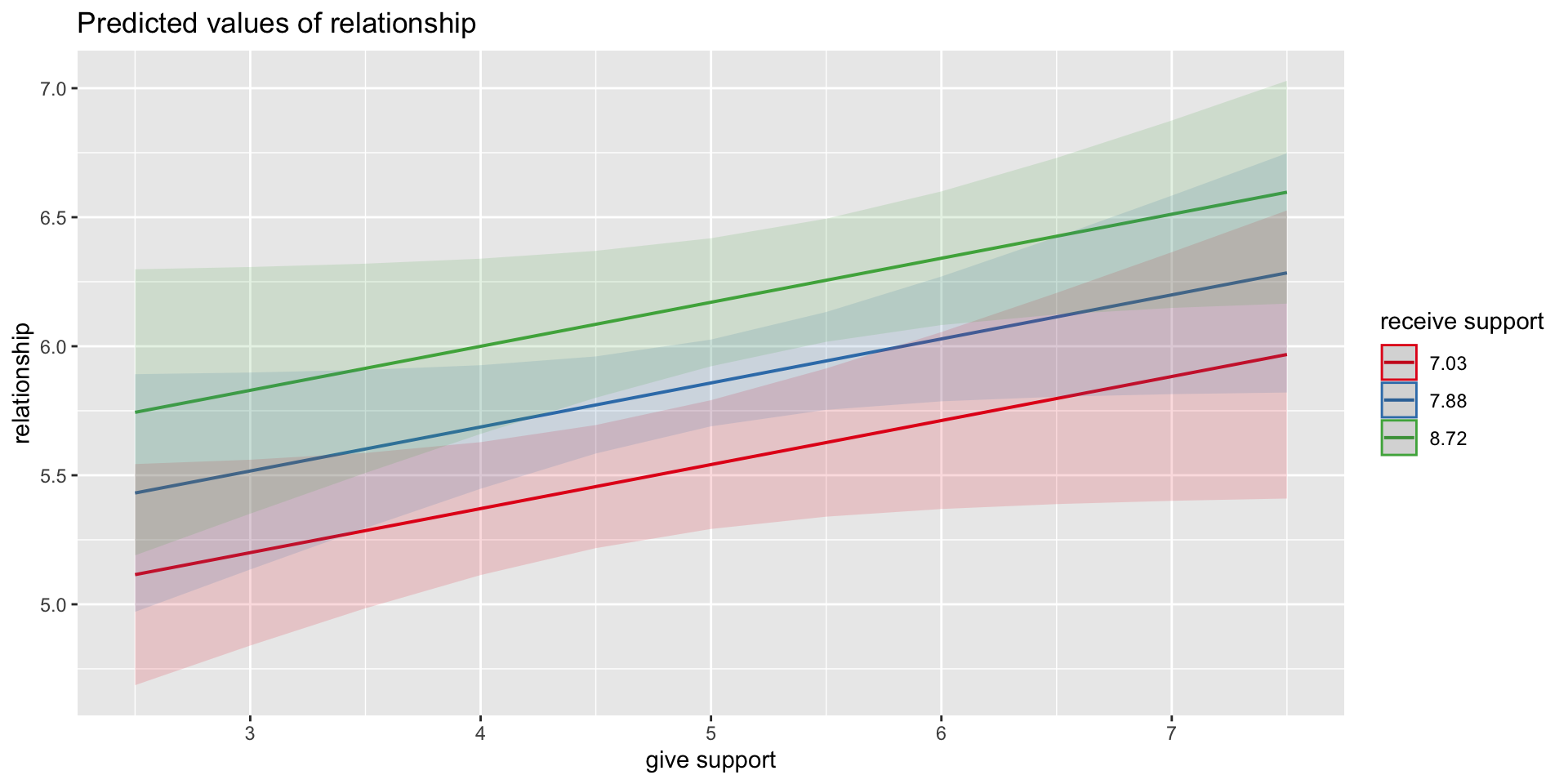
Even though the slope of one predictor, give_support, is less steep (accounting for less variance), the model overall captures more of the variability in Y (relationship quality).

un.model <- lm(relationship ~ give_support, data = support_df)
summary(un.model)

...
Residual standard error: 0.8073 on 76 degrees of freedom
Multiple R-squared:  0.1275,    Adjusted R-squared:  0.1161 
F-statistic: 11.11 on 1 and 76 DF,  p-value: 0.001329
...

mr.model <- lm(relationship ~ give_support + receive_support, data = support_df)
summary(mr.model)

...
Residual standard error: 0.7577 on 75 degrees of freedom
Multiple R-squared:  0.2416,    Adjusted R-squared:  0.2214 
F-statistic: 11.95 on 2 and 75 DF,  p-value: 0.00003128
...

Estimating model fit

mr.model <- lm(relationship ~ receive_support + give_support, data = support_df)
summary(mr.model)

Call:
lm(formula = relationship ~ receive_support + give_support, data = support_df)

Residuals:
     Min       1Q   Median       3Q      Max 
-2.26837 -0.40225  0.07701  0.42147  1.76074 

Coefficients:
                Estimate Std. Error t value Pr(>|t|)   
(Intercept)      2.07212    0.81218   2.551  0.01277 * 
receive_support  0.37216    0.11078   3.359  0.00123 **
give_support     0.17063    0.08785   1.942  0.05586 . 
---
Signif. codes:  0 '***' 0.001 '**' 0.01 '*' 0.05 '.' 0.1 ' ' 1

Residual standard error: 0.7577 on 75 degrees of freedom
Multiple R-squared:  0.2416,    Adjusted R-squared:  0.2214 
F-statistic: 11.95 on 2 and 75 DF,  p-value: 0.00003128

library(broom); library(scales)
support_df1 = augment(mr.model)
support_df1 %>%
  ggplot(aes(x = relationship, y = .fitted)) + geom_point() + geom_hline(aes(yintercept = mean(relationship), color = "bar(Y)")) + geom_smooth(method = "lm", aes(color = "R[bar(Y)][Y]")) + scale_x_continuous("Y (relationship)") + scale_color_discrete(labels = parse_format()) + scale_y_continuous(expression(hat(Y))) + theme_bw(base_size = 20)

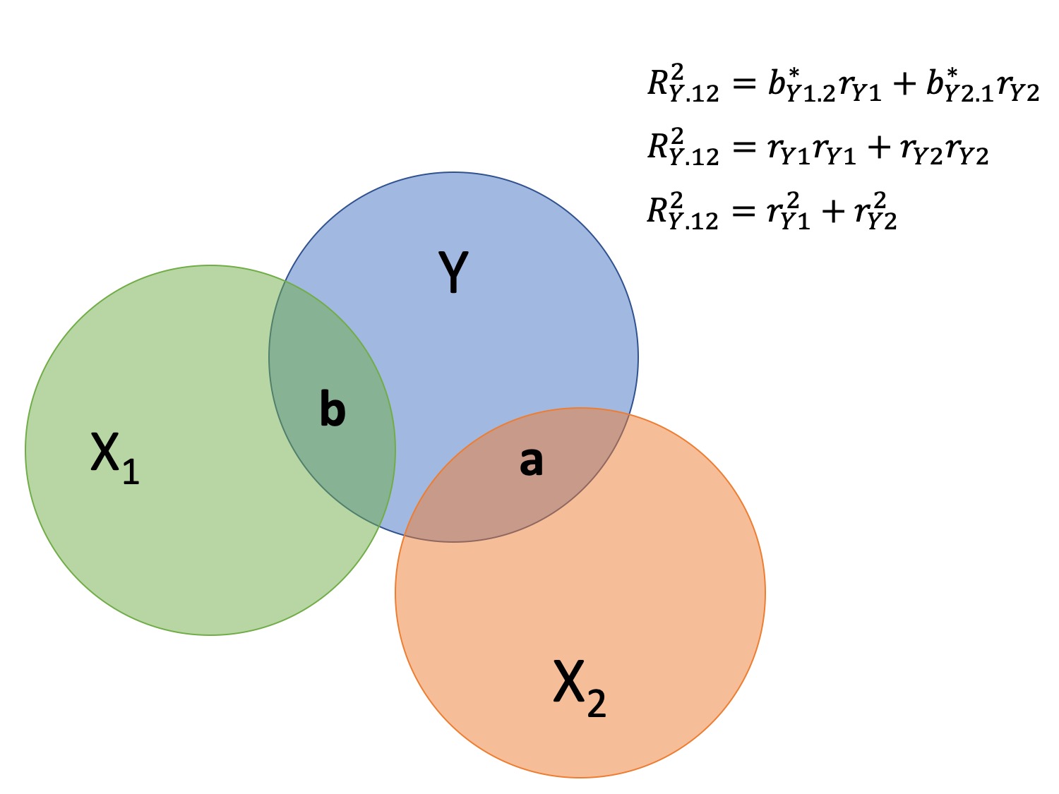
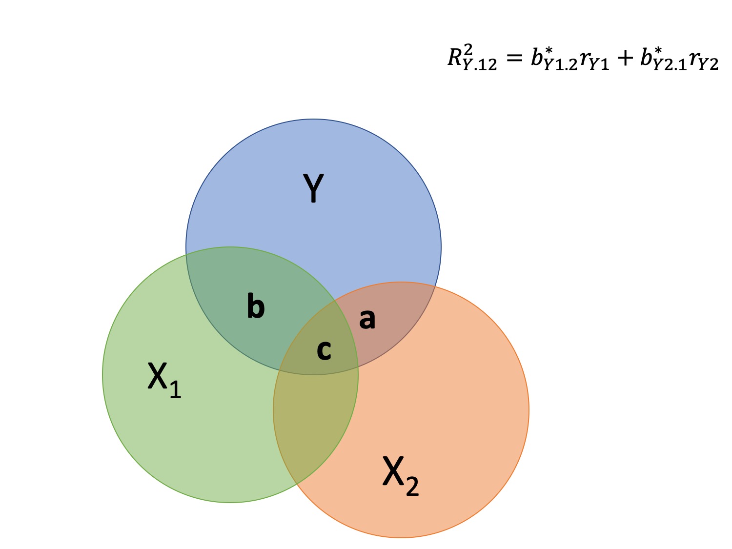
Multiple correlation, R

\[\large \hat{Y} = b_{0} + b_{1}X_{1} + b_{2}X_{2}\]

• \(\hat{Y}\) is a linear combination of Xs
• \(r_{Y\hat{Y}}\) = multiple correlation = R

\[\large R = \sqrt{b_{1}^*r_{Y1} + b_{2}^*r_{Y2}}\] \[\large R^2 = {b_{1}^*r_{Y1} + b_{2}^*r_{Y2}}\]

Decomposing sums of squares

We haven’t changed our method of decomposing variance from the univariate model

\[\Large \frac{SS_{regression}}{SS_{Y}} = R^2\] \[\Large {SS_{regression}} = R^2({SS_{Y})}\]

\[\Large {SS_{residual}} = (1- R^2){SS_{Y}}\]

significance tests

• \(R^2\) (omnibus)
  
• Regression Coefficients
  
• Increments to \(R^2\)

R-squared, \(R^2\)

• Same interpretation as before

• Adding predictors into your model will increase \(R^2\) – regardless of whether or not the predictor is significantly correlated with Y.

  • Think back to sampling error. If the population correlation, \(\rho\), is 0, will your sample estimate always be 0?

• Adjusted/Shrunken \(R^2\) takes into account the number of predictors in your model

Adjusted R-squared, \(\text{Adj } R^2\)

\[\large R_{A}^2 = 1 - (1 -R^2)\frac{n-1}{n-p-1}\]

• What happens if you add many IV’s to your model that are uncorrelated with your DV?

Adjusted R-squared, \(\text{Adj } R^2\)

\[\large R_{A}^2 = 1 - (1 -R^2)\frac{n-1}{n-p-1}\]

• What happens as you add more covariates to your model that are highly correlated with your key predictor, X?

\[b_{1}^* = \frac{r_{Y1}-r_{Y2}r_{12}}{1-r_{12}^2}\]

ANOVA

summary(mr.model)

Call:
lm(formula = relationship ~ receive_support + give_support, data = support_df)

Residuals:
     Min       1Q   Median       3Q      Max 
-2.26837 -0.40225  0.07701  0.42147  1.76074 

Coefficients:
                Estimate Std. Error t value Pr(>|t|)   
(Intercept)      2.07212    0.81218   2.551  0.01277 * 
receive_support  0.37216    0.11078   3.359  0.00123 **
give_support     0.17063    0.08785   1.942  0.05586 . 
---
Signif. codes:  0 '***' 0.001 '**' 0.01 '*' 0.05 '.' 0.1 ' ' 1

Residual standard error: 0.7577 on 75 degrees of freedom
Multiple R-squared:  0.2416,    Adjusted R-squared:  0.2214 
F-statistic: 11.95 on 2 and 75 DF,  p-value: 0.00003128

ANOVA

The omnibus test uses all SS associated with predictors.

anova(mr.model)

Analysis of Variance Table

Response: relationship
                Df Sum Sq Mean Sq F value    Pr(>F)    
receive_support  1 11.553 11.5528 20.1253 0.0000257 ***
give_support     1  2.166  2.1655  3.7724   0.05586 .  
Residuals       75 43.053  0.5740                      
---
Signif. codes:  0 '***' 0.001 '**' 0.01 '*' 0.05 '.' 0.1 ' ' 1

\[SS_{\text{model}} = 13.72\] \[MS_{\text{model}} = \frac{SS_{\text{model}}}{df_{\text{model}}} = 6.86\]

\[F_{\text{model}} = \frac{MS_{\text{model}}}{MS_{\text{residual}}} = 11.95\]

ANOVA

The omnibus test uses all SS associated with predictors.

anova(mr.model)

Analysis of Variance Table

Response: relationship
                Df Sum Sq Mean Sq F value    Pr(>F)    
receive_support  1 11.553 11.5528 20.1253 0.0000257 ***
give_support     1  2.166  2.1655  3.7724   0.05586 .  
Residuals       75 43.053  0.5740                      
---
Signif. codes:  0 '***' 0.001 '**' 0.01 '*' 0.05 '.' 0.1 ' ' 1

Note that the p-values in this table do NOT match the p-values in the regression summary table. For the time being, just know that, in a multiple regression framework, you should use the summary() output to interpret the unique contribution of predictors, not the anova() output. We’ll return to these calculations later in the term.

summary(mr.model)

...
receive_support  0.37216    0.11078   3.359  0.00123 **
give_support     0.17063    0.08785   1.942  0.05586 . 
...

Next time…

Standard errors of regression coefficients

Model comparisons

Categorical predictors