Interactions (V)

# Interactions (V)

---

## Reminder

Go to lab on Friday!!!

* Download LaTex before lab starts.

Homework 2 due on Monday (9 am)

---

## Last time...

Factorial ANOVA
* Estimated marginal means
* Estimated cell means
* Sums of squares

---

## ANOVA vs Regression

Interaction tests whether there are differences in differences.

**Simple main effect** -- the effect of Factor A at a specific level of Factor B
]
.pull-right[
### Regression

Interaction tests whether slope changes.

**Simple slopes** -- the slope of Variable A at a specific level of Variable B
]

---

```r
library(car) 
fit = lm(Time~Speed*Noise, data = Data)
summary(aov(fit))
```

```
##              Df  Sum Sq Mean Sq F value   Pr(>F)    
## Speed         2 2805871 1402936 109.397  < 2e-16 ***
## Noise         2  341315  170658  13.307 4.25e-06 ***
## Speed:Noise   4  295720   73930   5.765 0.000224 ***
## Residuals   171 2192939   12824                     
## ---
## Signif. codes:  0 '***' 0.001 '**' 0.01 '*' 0.05 '.' 0.1 ' ' 1
```

```r
Anova(fit, type = 2)
```

```
## Anova Table (Type II tests)
## 
## Response: Time
##              Sum Sq  Df  F value    Pr(>F)    
## Speed       2805871   2 109.3975 < 2.2e-16 ***
## Noise        341315   2  13.3075 4.252e-06 ***
## Speed:Noise  295720   4   5.7649 0.0002241 ***
## Residuals   2192939 171                       
## ---
## Signif. codes:  0 '***' 0.001 '**' 0.01 '*' 0.05 '.' 0.1 ' ' 1
```
---

```r
fit = lm(Time~Speed*Noise, data = Data)
summary(fit)
```

```
## 
## Call:
## lm(formula = Time ~ Speed * Noise, data = Data)
## 
## Residuals:
##     Min      1Q  Median      3Q     Max 
## -316.23  -70.82    4.99   79.87  244.40 
## 
## Coefficients:
##                                 Estimate Std. Error t value Pr(>|t|)    
## (Intercept)                       630.72      25.32  24.908  < 2e-16 ***
## SpeedMedium                      -105.44      35.81  -2.944  0.00369 ** 
## SpeedFast                        -301.45      35.81  -8.418 1.49e-14 ***
## NoiseControllable                 -54.05      35.81  -1.509  0.13305    
## NoiseUncontrollable               -36.28      35.81  -1.013  0.31243    
## SpeedMedium:NoiseControllable      21.48      50.64   0.424  0.67201    
## SpeedFast:NoiseControllable        12.01      50.64   0.237  0.81287    
## SpeedMedium:NoiseUncontrollable  -184.39      50.64  -3.641  0.00036 ***
## SpeedFast:NoiseUncontrollable     -24.84      50.64  -0.490  0.62448    
## ---
## Signif. codes:  0 '***' 0.001 '**' 0.01 '*' 0.05 '.' 0.1 ' ' 1
## 
## Residual standard error: 113.2 on 171 degrees of freedom
## Multiple R-squared:  0.6109,	Adjusted R-squared:  0.5927 
## F-statistic: 33.56 on 8 and 171 DF,  p-value: < 2.2e-16
```
---

```r
library(emmeans)
fit.grid = ref_grid(fit)
pairs(fit.grid, adjust = "holm")
```

```
##  contrast                                    estimate   SE  df t.ratio p.value
##  Slow,None - Medium,None                        105.4 35.8 171  2.944  0.0553 
##  Slow,None - Fast,None                          301.4 35.8 171  8.418  <.0001 
##  Slow,None - Slow,Controllable                   54.1 35.8 171  1.509  1.0000 
##  Slow,None - Medium,Controllable                138.0 35.8 171  3.854  0.0026 
##  Slow,None - Fast,Controllable                  343.5 35.8 171  9.592  <.0001 
##  Slow,None - Slow,Uncontrollable                 36.3 35.8 171  1.013  1.0000 
##  Slow,None - Medium,Uncontrollable              326.1 35.8 171  9.106  <.0001 
##  Slow,None - Fast,Uncontrollable                362.6 35.8 171 10.124  <.0001 
##  Medium,None - Fast,None                        196.0 35.8 171  5.473  <.0001 
##  Medium,None - Slow,Controllable                -51.4 35.8 171 -1.435  1.0000 
##  Medium,None - Medium,Controllable               32.6 35.8 171  0.910  1.0000 
##  Medium,None - Fast,Controllable                238.1 35.8 171  6.648  <.0001 
##  Medium,None - Slow,Uncontrollable              -69.2 35.8 171 -1.931  0.6615 
##  Medium,None - Medium,Uncontrollable            220.7 35.8 171  6.162  <.0001 
##  Medium,None - Fast,Uncontrollable              257.1 35.8 171  7.180  <.0001 
##  Fast,None - Slow,Controllable                 -247.4 35.8 171 -6.908  <.0001 
##  Fast,None - Medium,Controllable               -163.4 35.8 171 -4.564  0.0002 
##  Fast,None - Fast,Controllable                   42.0 35.8 171  1.174  1.0000 
##  Fast,None - Slow,Uncontrollable               -265.2 35.8 171 -7.405  <.0001 
##  Fast,None - Medium,Uncontrollable               24.7 35.8 171  0.689  1.0000 
##  Fast,None - Fast,Uncontrollable                 61.1 35.8 171  1.707  0.9867 
##  Slow,Controllable - Medium,Controllable         84.0 35.8 171  2.344  0.2627 
##  Slow,Controllable - Fast,Controllable          289.4 35.8 171  8.082  <.0001 
##  Slow,Controllable - Slow,Uncontrollable        -17.8 35.8 171 -0.496  1.0000 
##  Slow,Controllable - Medium,Uncontrollable      272.1 35.8 171  7.597  <.0001 
##  Slow,Controllable - Fast,Uncontrollable        308.5 35.8 171  8.615  <.0001 
##  Medium,Controllable - Fast,Controllable        205.5 35.8 171  5.738  <.0001 
##  Medium,Controllable - Slow,Uncontrollable     -101.7 35.8 171 -2.841  0.0707 
##  Medium,Controllable - Medium,Uncontrollable    188.1 35.8 171  5.252  <.0001 
##  Medium,Controllable - Fast,Uncontrollable      224.6 35.8 171  6.271  <.0001 
##  Fast,Controllable - Slow,Uncontrollable       -307.2 35.8 171 -8.579  <.0001 
##  Fast,Controllable - Medium,Uncontrollable      -17.4 35.8 171 -0.486  1.0000 
##  Fast,Controllable - Fast,Uncontrollable         19.1 35.8 171  0.533  1.0000 
##  Slow,Uncontrollable - Medium,Uncontrollable    289.8 35.8 171  8.093  <.0001 
##  Slow,Uncontrollable - Fast,Uncontrollable      326.3 35.8 171  9.111  <.0001 
##  Medium,Uncontrollable - Fast,Uncontrollable     36.5 35.8 171  1.018  1.0000 
## 
## P value adjustment: holm method for 36 tests
```

---

In `sjPlot()`, predicted values are the expected value of Y given all possible values of X, **at specific values of M**. If you don't give it all of M, it will choose every possible value.

```r
library(sjPlot)
plot_model(fit, type = "pred", 
           terms = c("Noise", "Speed")) + 
  theme_sjplot(base_size = 20) + 
  theme(legend.position = "bottom")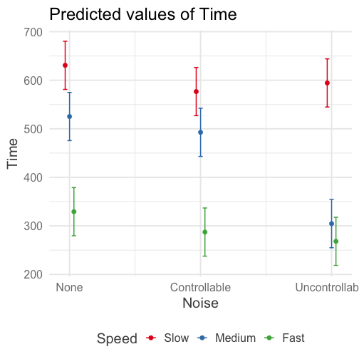
```

]

]
---

In `sjPlot()`, predicted values are the expected value of Y given all possible values of X, **at specific values of M**. If you don't specify levels of M, it will choose the lowest possible value.

```r
library(sjPlot)
plot_model(fit, type = "pred", 
           terms = c("Noise")) + 
  theme_sjplot(base_size = 20) + 
  theme(legend.position = "bottom")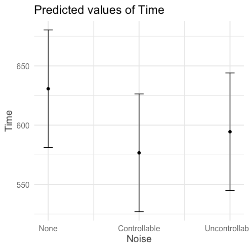
```

]

]---

In `sjPlot()`, predicted values are the expected value of Y given all possible values of X, **at specific values of M**. If you don't specify levels of M, it will choose the lowest possible value.

```r
library(sjPlot)
plot_model(fit, type = "pred", 
           terms = c("Noise", "Speed[Fast]")) + 
  theme_sjplot(base_size = 20) + 
  theme(legend.position = "bottom")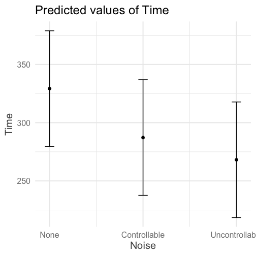
```

]

]

---

In `sjPlot()`, estimated marginal means are the expected value of Y given all possible values of X, **ignoring M**.

```r
library(sjPlot)
plot_model(fit, type = "emm", 
           terms = c("Noise")) + 
  theme_sjplot(base_size = 20) + 
  theme(legend.position = "bottom")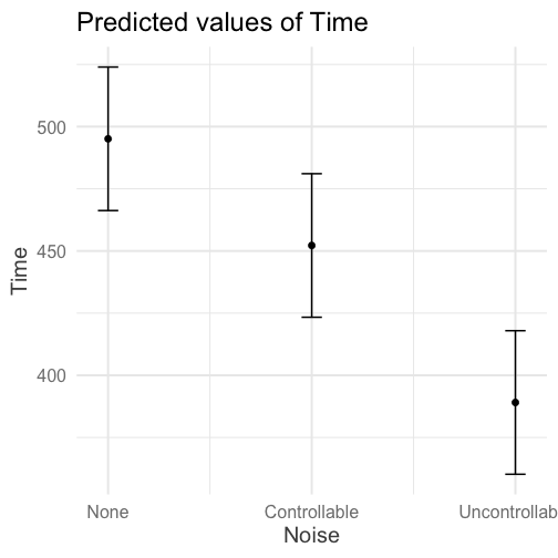
```

]

]

---

## Power

The likelihood of finding an effect *if the effect actually exists.* Power gets larger as we:
* increase our sample size
* reduce (error) variance
* raise our Type I error rate
* study larger effects

---

![](18-interactions_files/figure-html/unnamed-chunk-10-1.png)

---

## Power in multiple regression (additive effects)

When calculating power for the omnibus test, use the expected multiple `$R^2$` value to calculate an effect size:

`$$\large f^2 = \frac{R^2}{1-R^2}$$`
---

### Omnibus power

```r
R2 = .10
(f = R2/(1-R2))
```

```
## [1] 0.1111111
```

```r
library(pwr)
pwr.f2.test(u = 3, # number of predictors in the model
            f2 = f, 
            sig.level = .05, #alpha
            power =.90) # desired power
```

```
## 
##      Multiple regression power calculation 
## 
##               u = 3
##               v = 127.5235
##              f2 = 0.1111111
##       sig.level = 0.05
##           power = 0.9
```

`v` is the denominator df of freedom, so the number of participants needed is v + p + 1.

---

### Coefficient power

To estimate power for a single coefficient, you need to consider (1) how much variance is accounted for by just the variable and (2) how much variance you'll account for in Y overall.

`$$\large f^2 = \frac{R^2_Y-R^2_{Y.X}}{1-R_Y^2}$$`
---
### Coefficient power

```r
R2 = .10
RX1 = .03
(f = (R2-RX1)/(1-R2))
```

```
## [1] 0.07777778
```

```r
pwr.f2.test(u = 3, # number of predictors in the model
            f2 = f, 
            sig.level = .05, #alpha
            power =.90) # desired power
```

```
## 
##      Multiple regression power calculation 
## 
##               u = 3
##               v = 182.1634
##              f2 = 0.07777778
##       sig.level = 0.05
##           power = 0.9
```

`v` is the denominator df of freedom, so the number of participants needed is v + p + 1.
---

## Effect sizes (interactions)

To start our discussion on powering interaction terms, we need to first consider the effect size of an interaction.

How big can we reasonably expect an interaction to be?

- Interactions are always partialled effects; that is, we examine the relationship between the product of variables X and Z only after we have controlled for X and controlled for Z. How does this affect the size of the relationship between XZ and Y?

???

The effect of XZ and Y will be made smaller as X or Z (or both) is related to the product -- the semi-partial correlation is always smaller than or equal to the zero-order correlation.

---

## McClelland and Judd (1993)

Is it more difficult to find interaction effects in experimental studies or observational studies?

What factors make it relatively easier to find interactions in experimental work?

---

### Factors influencing power in experimental studies

- No measurement error of IV 
    * don't have to guess what condition a participant is in
    * measurement error is exacerbated when two variables measured with error are multiplied by each other
    
- Experimentalists are more likely to find cross-over interactions; observational studies may be restricted to fan interactions
    * cross-over interactions are easier to detect than fan interactions
    
---

### Factors influencing power in experimental studies

- Experimentalists can concentrate scores on extreme ends on both X and Z
    * in observational studies, data tends to cluster around the mean 
    * increases variability in both X and Z, and in XZ

- Experimentalists can also force orthognality in X and Z

- Experimentalists can study the full range of X in an experiment

---

### McClelland and Judd's simulation

For the experiment simulations, we used 2 X 2 factorial designs, with values of X and Z equal to +1 and —1 and an equal number of observations at each of the four combinations of X and Z values.

```r
X = rep(c(-1,1), each = 50)
Z = rep(c(-1,1), times = 50)
table(X,Z)
```

```
##     Z
## X    -1  1
##   -1 25 25
##   1  25 25
```

---

### McClelland and Judd's simulation

For the field study simulations, we used values of X and Z that varied between the extreme values of +1 and —1. More specifically, in the field study simulations, values of X and Z were each sampled independently from a normal distribution with a mean of 0 and a standard deviation of 0.5. Values of X and Z were rounded to create equally spaced 9-point scales ranging from -1 to +1 because ranges in field studies are always finite and because ratings are often on scales with discrete intervals.

```r
X = rnorm(n = 100, mean = 0, sd = .5)
Z = rnorm(n = 100, mean = 0, sd = .5)
X = round(X/.2)*.2
Z = round(Z/.2)*.2

psych::describe(data.frame(X,Z), fast = T)
```

```
##   vars   n  mean   sd min max range   se
## X    1 100 -0.07 0.54  -2 1.2   3.2 0.05
## Z    2 100  0.06 0.50  -1 1.4   2.4 0.05
```
---

For the simulations of both the field studies and the experiments, `$\beta_0 = 0, \beta_X=\beta_Z=\beta_{XZ} = 1.$` There were 100 observations, and errors for the model were sampled from the same normal distribution with a mean of 0 and a standard deviation of 4.

```r
Y = 0 + 1*X + 1*Z + 1*X*Z + rnorm(n = 100, mean = 0, sd = 4)
summary(lm(Y ~ X*Z))
```

```
## 
## Call:
## lm(formula = Y ~ X * Z)
## 
## Residuals:
##      Min       1Q   Median       3Q      Max 
## -11.0032  -3.3243   0.0476   2.3725  10.1094 
## 
## Coefficients:
##             Estimate Std. Error t value Pr(>|t|)  
## (Intercept)  -0.3081     0.4333  -0.711   0.4788  
## X             1.0976     0.8128   1.350   0.1800  
## Z             1.8033     0.8491   2.124   0.0363 *
## X:Z           2.0854     1.5353   1.358   0.1775  
## ---
## Signif. codes:  0 '***' 0.001 '**' 0.01 '*' 0.05 '.' 0.1 ' ' 1
## 
## Residual standard error: 4.248 on 96 degrees of freedom
## Multiple R-squared:  0.0697,	Adjusted R-squared:  0.04062 
## F-statistic: 2.397 on 3 and 96 DF,  p-value: 0.07282
```

---

From 100 simulations each, estimates of the model parameter `$\beta_{XZ}$` the moderator or interaction effect equaled 0.977 and 0.979 for the field studies and experiments, respectively.

```r
set.seed(0305)
```

```r
# for experimental studies
sim = 100
ebeta_xz = numeric(length = 100)
et_xz = numeric(length = 100)
for(i in 1:sim){
  # simulate data
  X = rep(c(-1,1), each = 50)
  Z = rep(c(-1,1), times = 50)
 
  
   Y = 0 + 1*X + 1*Z + 1*X*Z + 
    rnorm(n = 100, mean = 0, sd = 4)
  #run model
  model = lm(Y ~ X*Z)
  coef = coef(summary(model))
  #extract coefficients
  beta = coef["X:Z", "Estimate"]
  t_val = coef["X:Z", "t value"]
  #save to vectors
  ebeta_xz[i] = beta
  et_xz[i] = t_val
}
```
]
.pull-right[

```r
# for observational studies

obeta_xz = numeric(length = 100)
ot_xz = numeric(length = 100)
for(i in 1:sim){
  # simulate data
  X = rnorm(n = 100, mean=0, sd = .5)
  Z = rnorm(n = 100, mean=0, sd = .5)
  X = round(X/.2)*.2
  Z = round(Z/.2)*.2
  Y = 0 + 1*X + 1*Z + 1*X*Z + 
    rnorm(n = 100, mean = 0, sd = 4)
  #run model
  model = lm(Y ~ X*Z)
  coef = coef(summary(model))
  #extract coefficients
  beta = coef["X:Z", "Estimate"]
  t_val = coef["X:Z", "t value"]
  #save to vectors
  obeta_xz[i] = beta
  ot_xz[i] = t_val
}
```
]
---

```r
mean(ebeta_xz)
```

```
## [1] 0.9440304
```

```r
mean(obeta_xz)
```

```
## [1] 1.175444
```

![](18-interactions_files/figure-html/unnamed-chunk-20-1.png)

---

```r
mean(et_xz)
```

```
## [1] 2.383435
```

```r
mean(ot_xz)
```

```
## [1] 0.7411209
```

![](18-interactions_files/figure-html/unnamed-chunk-22-1.png)

---

```r
cv = qt(p = .975, df = 100-3-1)
esig = et_xz > cv
sum(esig)
```

```
## [1] 66
```

```r
osig = ot_xz > cv
sum(osig)
```

```
## [1] 12
```

In our simulation, 66% of experimental studies were statistically significant, whereas only 12% of observational studies were significant. Remember, we built our simulation based on data where there really is an interaction effect (i.e., the null is false).

McClelland and Judd found that 74% of experimental studies and 9% of observational studies were significant.

---

### Efficiency

???
Efficiency = the ratio of the variance of XZ (controlling for X and Z) of a design to the best possible design (upper right corner). High efficiency is better; best efficiency is 1.

---

### Efficiency

.pull-left[
If the optimal design has N obserations, then to have the same standard error (i.e., the same power), any other design needs to have N*(1/efficency).

So a design with .06 efficency needs `$\frac{1}{.06} = 16.67$` times the sample size to detect the effect. 
]

This particular point has been ["rediscovered"](https://statmodeling.stat.columbia.edu/2018/03/15/need-16-times-sample-size-estimate-interaction-estimate-main-effect/) as recently as 2018:

* you need 16 times the sample size to detect an interaction as you need for a main effect of the same size.

???

This generalizes to higher-order interactions as well. If you have a three-way interaction, you need 16*16 (256 times the number of people).

---

## Observational studies: What NOT to do

Recode X and Z into more extreme values (e.g., median splits)
    * while this increases variance in X and Z, it also increases measurement error

Collect a random sample and then only perform analyses on the subsample with extreme values
    * reduces sample size and also generalizability
    
#### What can be done?
M&J suggest oversampling extremes and using weighted and unweighted samples

---

## Experimental studies: What NOT to do

Be mean to field researchers

Forget about lack of external validity and generalizability

Ignore power when comparing interaction between covariate and experimental predictors (ANCOVA or multiple regression with categorical and continuous predictors)

---

## Non-linear relationships

Linear lines often make bad predictions -- very few processes that we study actually have linear relationships. For example, effort had diminishing returns (e.g., log functions), or small advantages early in life can have significant effects on mid-life outcones (e.g., exponentional functions). In cases where the direction of the effect is constant but changing in magnitude, the best way to handle the data is to transform a variable (usually the outcome) and run linear analyses.

```r
log_y = ln(y)
lm(log_y ~ x)
```
---

## Polynomial relationships

Other processes represent changes in the directon of relationship -- for example, it is believed that a small amount of anxiety is benefitial for performance on some tasks (positive direction) but too much is detrimental (negative direction). When the shape of the effect includes change(s) in direction, then a polynomial term(s) may be more appropriate.

It should be noted that polynomials are often a poor approximation for a non-linear effect of X on Y. However, correctly testing for non-linear effects usually requires (a) a lot of data and (b) making a number of assumptions about the data. Polynomial regression can be a useful tool for exploratory analysis and in cases when data are limited in terms of quantity and/or quality.

---
## Polynomial regression 
 
Polynomial regression is most often a form of hierarchical regressoin that systematically tests a series of higher order functions for a single variable.

$$
`\begin{aligned}
\large \textbf{Linear: } \hat{Y} &= b_0 + b_1X \\
\large \textbf{Quadtratic: } \hat{Y} &= b_0 + b_1X + b_2X^2 \\
\large \textbf{Cubic: } \hat{Y} &= b_0 + b_1X + b_2X^2 + b_3X^3\\
\end{aligned}`
$$

---
### Example

Can a team have too much talent? Researchers hypothesized that teams with too many talented players have poor intrateam coordination and therefore perform worse than teams with a moderate amount of talent. To test this hypothesis, they looked at 208 international football teams. Talent was the percentage of players during the 2010 and 2014 World Cup Qualifications phases who also had contracts with elite club teams. Performance was the number of points the team earned during these same qualification phases.

```r
library(here)
football = read.csv(here("data/swaab.csv"))
```

.small[Swaab, R.I., Schaerer, M, Anicich, E.M., Ronay, R., and Galinsky, A.D. (2014). [The too-much-talent effect: Team
interdependence determines when more talent is too much or not enough.](https://www8.gsb.columbia.edu/cbs-directory/sites/cbs-directory/files/publications/Too%20much%20talent%20PS.pdf) _Psychological Science 25_(8), 1581-1591.]

---
.pull-left[

```r
head(football)
```

```
##       country points talent
## 1       Spain   1485     85
## 2     Germany   1300     76
## 3      Brazil   1242     48
## 4    Portugal   1189     16
## 5   Argentina   1175     35
## 6 Switzerland   1149      9
```
]
.pull-right[

```r
ggplot(football, aes(x = talent, y = points)) +
  geom_point() + 
  geom_smooth(se = F) +
  theme_bw(base_size = 20)
```

```
## `geom_smooth()` using method = 'loess' and formula 'y ~ x'
```

![](18-interactions_files/figure-html/unnamed-chunk-28-1.png)

]

---

```r
mod1 = lm(points ~ talent, data = football)
library(broom)
aug1 = augment(mod1)
ggplot(aug1, aes(x = .fitted, y = .resid)) +
  geom_point() + 
  geom_smooth(se = F) +
  theme_bw(base_size = 20)
```

![](18-interactions_files/figure-html/mod1-1.png)

---

```r
mod2 = lm(points ~ talent + I(talent^2), data = football)
summary(mod2)
```

```
## 
## Call:
## lm(formula = points ~ talent + I(talent^2), data = football)
## 
## Residuals:
##     Min      1Q  Median      3Q     Max 
## -384.66 -193.82  -35.34  152.11  729.66 
## 
## Coefficients:
##              Estimate Std. Error t value Pr(>|t|)    
## (Intercept) 305.34402   17.62668  17.323  < 2e-16 ***
## talent       54.89787    5.46864  10.039  < 2e-16 ***
## I(talent^2)  -0.57022    0.07499  -7.604 1.01e-12 ***
## ---
## Signif. codes:  0 '***' 0.001 '**' 0.01 '*' 0.05 '.' 0.1 ' ' 1
## 
## Residual standard error: 236.3 on 205 degrees of freedom
## Multiple R-squared:  0.4644,	Adjusted R-squared:  0.4592 
## F-statistic: 88.87 on 2 and 205 DF,  p-value: < 2.2e-16
```

---

```r
library(sjPlot)
plot_model(mod2, type = "pred")
```

```
## $talent
```

![](18-interactions_files/figure-html/unnamed-chunk-29-1.png)

---
## Interpretation

The intercept is the predicted value of Y when x = 0 -- this is always the interpretation of the intercept, no matter what kind of regression model you're running.

The `$b_1$` coefficient is the tangent to the curve when X=0. In other words, this is the rate of change when X is equal to 0. If 0 is not a meaningful value on your X, you may want to center, as this will tell you the rate of change at the mean of X.

```r
football$talent_c50 = football$talent - 50
mod2_50 = lm(points ~ talent_c50 + I(talent_c50^2), data = football)
```

---

```r
summary(mod2_50)
```

```
## 
## Call:
## lm(formula = points ~ talent_c50 + I(talent_c50^2), data = football)
## 
## Residuals:
##     Min      1Q  Median      3Q     Max 
## -384.66 -193.82  -35.34  152.11  729.66 
## 
## Coefficients:
##                   Estimate Std. Error t value Pr(>|t|)    
## (Intercept)     1624.68872   97.18998  16.717  < 2e-16 ***
## talent_c50        -2.12408    2.56568  -0.828    0.409    
## I(talent_c50^2)   -0.57022    0.07499  -7.604 1.01e-12 ***
## ---
## Signif. codes:  0 '***' 0.001 '**' 0.01 '*' 0.05 '.' 0.1 ' ' 1
## 
## Residual standard error: 236.3 on 205 degrees of freedom
## Multiple R-squared:  0.4644,	Adjusted R-squared:  0.4592 
## F-statistic: 88.87 on 2 and 205 DF,  p-value: < 2.2e-16
```

---

```
## $talent_c50
```

![](18-interactions_files/figure-html/unnamed-chunk-32-1.png)
---

Or you can choose another value to center your predictor on, if there's a value that has a particular meaning or interpretation.

```r
football$talent_c = football$talent - mean(football$talent)
mod2_c = lm(points ~ talent_c + I(talent_c^2), data = football)
```

---

```r
mean(football$talent)
```

```
## [1] 3.216346
```

```r
summary(mod2_c)
```

```
## 
## Call:
## lm(formula = points ~ talent_c + I(talent_c^2), data = football)
## 
## Residuals:
##     Min      1Q  Median      3Q     Max 
## -384.66 -193.82  -35.34  152.11  729.66 
## 
## Coefficients:
##                Estimate Std. Error t value Pr(>|t|)    
## (Intercept)   476.01572   19.94656  23.865  < 2e-16 ***
## talent_c       51.22982    5.00212  10.242  < 2e-16 ***
## I(talent_c^2)  -0.57022    0.07499  -7.604 1.01e-12 ***
## ---
## Signif. codes:  0 '***' 0.001 '**' 0.01 '*' 0.05 '.' 0.1 ' ' 1
## 
## Residual standard error: 236.3 on 205 degrees of freedom
## Multiple R-squared:  0.4644,	Adjusted R-squared:  0.4592 
## F-statistic: 88.87 on 2 and 205 DF,  p-value: < 2.2e-16
```

---

```
## $talent_c
```

![](18-interactions_files/figure-html/unnamed-chunk-35-1.png)
---

## Interpretation

The `$b_2$` coefficient indexes the acceleration, which is how much the slope is going to change. More specifically, `$2 \times b_2$` is the acceleration: the rate of change in `$b_1$` for a 1-unit change in X.

You can use this to calculate the slope of the tangent line at any value of X you're interested in:
`$$\large b_1 + (2\times b_2\times X)$$`

---

```r
tidy(mod2)
```

```
## # A tibble: 3 x 5
##   term        estimate std.error statistic  p.value
##   <chr>          <dbl>     <dbl>     <dbl>    <dbl>
## 1 (Intercept)  305.      17.6        17.3  5.22e-42
## 2 talent        54.9      5.47       10.0  1.53e-19
## 3 I(talent^2)   -0.570    0.0750     -7.60 1.01e-12
```

```r
54.9 + (2*-.570*10)
```

```
## [1] 43.5
```

]
.pull-right[
**At X = 70**

```r
54.9 + (2*-.570*70)
```

```
## [1] -24.9
```

]

---

## Polynomials are interactions

An term for `$X^2$` is a term for `$X \times X$` or the multiplication of two independent variables holding the same values.

```r
football$talent_2 = football$talent*football$talent
tidy(lm(points ~ talent + talent_2, data = football))
```

```
## # A tibble: 3 x 5
##   term        estimate std.error statistic  p.value
##   <chr>          <dbl>     <dbl>     <dbl>    <dbl>
## 1 (Intercept)  305.      17.6        17.3  5.22e-42
## 2 talent        54.9      5.47       10.0  1.53e-19
## 3 talent_2      -0.570    0.0750     -7.60 1.01e-12
```
---

## Polynomials are interactions

Put another way:

`$$\large \hat{Y} = b_0 + b_1X + b_2X^2$$`

`$$\large \hat{Y} = b_0 + \frac{b_1}{2}X + \frac{b_1}{2}X + b_2(X \times X)$$`

The interaction term in another model would be interpreted as "how does the slope of X change as I move up in Z?" -- here, we ask "how does the slope of X change as we move up in X?"
---

## When should you use polynomial terms?

You may choose to fit a polynomial term after looking at a scatterplot of the data or looking at residual plots. A U-shaped curve may be indicative that you need to fit a quadratic form -- although, as we discussed before, you may actually be measuring a different kind of non-linear relationship.

Polynomial terms should mostly be dictated by theory -- if you don't have a good reason for thinking there will be a change in sign, then a polynomial is not right for you.

And, of course, if you fit a polynomial regression, be sure to once again check your diagnostics before interpreting the coefficients. 
---

```r
aug2 = augment(mod2)
ggplot(aug2, aes(x = .fitted, y = .resid)) +
  geom_point() + 
  geom_smooth(se = F) +
  theme_bw(base_size = 20)
```

![](18-interactions_files/figure-html/unnamed-chunk-40-1.png)

---

```r
plot_model(mod2, type = "pred", show.data = T)
```

```
## $talent
```

![](18-interactions_files/figure-html/unnamed-chunk-41-1.png)

---

## Three-way interactions and beyond

---

### Three-way interactions (regression)

**Regression equation**

`$$\hat{Y} = b_{0} + b_{1}X + b_{2}Z + b_{3}W + b_{4}XZ + b_{5}XW + b_{6}ZW + b_{7}XZW$$`
The three-way interaction qualifies the three main effects (and any two-way interactions).

Like a two-way interaction, the three-way interaction is a conditional effect.  And it is symmetrical, meaning there are several equally correct ways of interpreting it.

**Factorial ANOVA**

We describe the factorial ANOVA design by the number of levels of each factor. "X by Z by W" (e.g., 2 by 3 by 4, or 2x3x4)
---
A two-way  (A x B) interaction means that the magnitude of one main effect (e.g., A main effect) depends on levels of the other variable (B).  But, it is equally correct to say that the magnitude of the B main effect depends on levels of A. In regression, we refer to these as **conditional effects** and in ANOVA, they are called **simple main effects.**

A three-way interaction means that the magnitude of one two-way interaction (e.g., A x B) depends on levels of the remaining variable (C).

It is equally correct to say that the magnitude of the A x C interaction depend on levels of B. Or, that the magnitude of the B x C interaction depends on levels of A. These are known as **simple interaction effects**.

---
### Example (regression)

```r
psych::describe(stress_data, fast = T)
```

```
## Warning in FUN(newX[, i], ...): no non-missing arguments to min; returning Inf
```

```
## Warning in FUN(newX[, i], ...): no non-missing arguments to max; returning -Inf
```

```
##         vars   n  mean    sd min  max range   se
## gender     1 150   NaN    NA Inf -Inf  -Inf   NA
## bad_day    2 150  2.95  1.29   1    5     4 0.11
## talk       3 150  2.57  1.20   1    5     4 0.10
## stress     4 150 30.15 10.00   1   51    50 0.82
```

```r
table(stress_data$gender)
```

```
## 
## female   male 
##     67     83
```

---

```r
mod_stress = lm(stress ~ bad_day*talk*gender, data = stress_data)
summary(mod_stress)
```

```
## 
## Call:
## lm(formula = stress ~ bad_day * talk * gender, data = stress_data)
## 
## Residuals:
##      Min       1Q   Median       3Q      Max 
## -10.6126  -3.2974   0.0671   3.1129  10.7774 
## 
## Coefficients:
##                         Estimate Std. Error t value Pr(>|t|)    
## (Intercept)              20.3385     4.5181   4.502 1.39e-05 ***
## bad_day                   2.5273     1.6596   1.523  0.13003    
## talk                      2.4870     1.3234   1.879  0.06227 .  
## gendermale               -0.1035     5.7548  -0.018  0.98568    
## bad_day:talk             -1.4220     0.4564  -3.116  0.00222 ** 
## bad_day:gendermale       -0.1244     2.0069  -0.062  0.95067    
## talk:gendermale           1.9797     2.2823   0.867  0.38718    
## bad_day:talk:gendermale   1.5260     0.7336   2.080  0.03931 *  
## ---
## Signif. codes:  0 '***' 0.001 '**' 0.01 '*' 0.05 '.' 0.1 ' ' 1
## 
## Residual standard error: 4.733 on 142 degrees of freedom
## Multiple R-squared:  0.7865,	Adjusted R-squared:  0.776 
## F-statistic: 74.72 on 7 and 142 DF,  p-value: < 2.2e-16
```

---

```r
library(reghelper)
simple_slopes(mod_stress)
```

```
##     bad_day     talk gender Test Estimate Std. Error t value  df  Pr(>|t|) Sig.
## 1  1.661455 1.365903 sstest        5.8571     1.7437  3.3590 142 0.0010045   **
## 2  2.953333 1.365903 sstest        8.3892     1.5671  5.3535 142 3.386e-07  ***
## 3  4.245211 1.365903 sstest       10.9214     2.5606  4.2651 142 3.627e-05  ***
## 4  1.661455 2.566667 sstest       11.2788     1.4571  7.7406 142 1.687e-12  ***
## 5  2.953333 2.566667 sstest       16.1781     1.0985 14.7274 142 < 2.2e-16  ***
## 6  4.245211 2.566667 sstest       21.0775     1.6775 12.5647 142 < 2.2e-16  ***
## 7  1.661455 3.767431 sstest       16.7004     2.3888  6.9912 142 9.806e-11  ***
## 8  2.953333 3.767431 sstest       23.9670     1.4830 16.1608 142 < 2.2e-16  ***
## 9  4.245211 3.767431 sstest       31.2335     2.0578 15.1784 142 < 2.2e-16  ***
## 10 1.661455   sstest female        0.1245     0.7221  0.1724 142 0.8633621     
## 11 2.953333   sstest female       -1.7125     0.5996 -2.8558 142 0.0049366   **
## 12 4.245211   sstest female       -3.5495     0.9450 -3.7561 142 0.0002511  ***
## 13   sstest 1.365903 female        0.5850     1.0725  0.5455 142 0.5862803     
## 14   sstest 2.566667 female       -1.1224     0.6181 -1.8160 142 0.0714796    .
## 15   sstest 3.767431 female       -2.8299     0.4630 -6.1115 142 9.006e-09  ***
## 16 1.661455   sstest   male        4.6396     1.0195  4.5510 142 1.137e-05  ***
## 17 2.953333   sstest   male        4.7741     0.6463  7.3862 142 1.177e-11  ***
## 18 4.245211   sstest   male        4.9085     0.9474  5.1813 142 7.418e-07  ***
## 19   sstest 1.365903   male        2.5451     0.5036  5.0533 142 1.315e-06  ***
## 20   sstest 2.566667   male        2.6700     0.6116  4.3655 142 2.427e-05  ***
## 21   sstest 3.767431   male        2.7950     1.2025  2.3244 142 0.0215233    *
```

---

```r
plot_model(mod_stress, type = "int", mdrt.values = "meansd")
```

![](18-interactions_files/figure-html/unnamed-chunk-46-1.png)

---

As a reminder, centering will change all but the highest-order terms in a model.

```r
stress_data = stress_data %>%
  mutate(bad_day_c = bad_day - mean(bad_day),
         talk_c = talk - mean(talk))
newmod = lm(stress ~ bad_day_c*talk_c*gender, data = stress_data)
```

---

```r
tidy(mod_stress)
```

```
## # A tibble: 8 x 5
##   term                    estimate std.error statistic   p.value
##   <chr>                      <dbl>     <dbl>     <dbl>     <dbl>
## 1 (Intercept)               20.3       4.52     4.50   0.0000139
## 2 bad_day                    2.53      1.66     1.52   0.130    
## 3 talk                       2.49      1.32     1.88   0.0623   
## 4 gendermale                -0.104     5.75    -0.0180 0.986    
## 5 bad_day:talk              -1.42      0.456   -3.12   0.00222  
## 6 bad_day:gendermale        -0.124     2.01    -0.0620 0.951    
## 7 talk:gendermale            1.98      2.28     0.867  0.387    
## 8 bad_day:talk:gendermale    1.53      0.734    2.08   0.0393
```

```r
tidy(newmod)
```

```
## # A tibble: 8 x 5
##   term                        estimate std.error statistic  p.value
##   <chr>                          <dbl>     <dbl>     <dbl>    <dbl>
## 1 (Intercept)                    23.4      0.845     27.7  3.89e-59
## 2 bad_day_c                      -1.12     0.618     -1.82 7.15e- 2
## 3 talk_c                         -1.71     0.600     -2.86 4.94e- 3
## 4 gendermale                     16.2      1.10      14.7  2.20e-30
## 5 bad_day_c:talk_c               -1.42     0.456     -3.12 2.22e- 3
## 6 bad_day_c:gendermale            3.79     0.870      4.36 2.47e- 5
## 7 talk_c:gendermale               6.49     0.882      7.36 1.38e-11
## 8 bad_day_c:talk_c:gendermale     1.53     0.734      2.08 3.93e- 2
```

---
### Four-way?

$$
`\begin{aligned}
\hat{Y} &= b_0 + b_1X + b_{2}Z + b_{3}W + b_{4}Q + b_{5}XW\\
&+ b_{6}ZW + b_{7}XZ + b_{8}QX + b_{9}QZ + b_{10}QW\\
&+ b_{11}XZQ + b_{12}XZW + b_{13}XWQ + b_{14}ZWQ + b_{15}XZWQ\\
\end{aligned}`
$$

3-way (and higher) interactions are incredibly difficult to interpret, in part because they represent incredibly complicated processes. If you have a solid theoretical rationale for conducting a 3-day interaction, be sure you've collected enough subjects to power your test (more on this later).

---

Especially with small samples, three-way interactions may be the result of a few outliers skewing a regression line. If you have stumbled upon a three-way interactoin during exploratory analyses, **be careful.** This is far more likely to be a result of over-fitting than uncovering a true underlying process.

Best practice for 3-way (and higher) interactions is to use at least one nominal moderator (ideally with only 2 levels), instead of all continuous moderators. This allows you to examine the 2-way interaction at each level of the nominal moderator.

Even better if one of these moderators is experimenter manipulated, which increases the likelihood of balanced conditions.

---

## Next time...

Statistical power and wrapping up interactions