class: center, middle, inverse, title-slide # Bootstrapping --- #Last time... Wrapping up interactions * Power # Today Finish polynomials and 3-way interactions Robust estimation * Weighted Least Squares * Boostrapping --- ## Polynomial regression Polynomial regression is most often a form of hierarchical regressoin that systematically tests a series of higher order functions for a single variable. $$ `\begin{aligned} \large \textbf{Linear: } \hat{Y} &= b_0 + b_1X \\ \large \textbf{Quadtratic: } \hat{Y} &= b_0 + b_1X + b_2X^2 \\ \large \textbf{Cubic: } \hat{Y} &= b_0 + b_1X + b_2X^2 + b_3X^3\\ \end{aligned}` $$ --- ### Example Can a team have too much talent? Researchers hypothesized that teams with too many talented players have poor intrateam coordination and therefore perform worse than teams with a moderate amount of talent. To test this hypothesis, they looked at 208 international football teams. Talent was the percentage of players during the 2010 and 2014 World Cup Qualifications phases who also had contracts with elite club teams. Performance was the number of points the team earned during these same qualification phases. ```r library(here) football = read.csv(here("data/swaab.csv")) ``` .small[Swaab, R.I., Schaerer, M, Anicich, E.M., Ronay, R., and Galinsky, A.D. (2014). [The too-much-talent effect: Team interdependence determines when more talent is too much or not enough.](https://www8.gsb.columbia.edu/cbs-directory/sites/cbs-directory/files/publications/Too%20much%20talent%20PS.pdf) _Psychological Science 25_(8), 1581-1591.] --- ```r mod1 = lm(points ~ talent, data = football) library(broom) aug1 = augment(mod1) ggplot(aug1, aes(x = .fitted, y = .resid)) + geom_point() + geom_smooth(se = F) + theme_bw(base_size = 20) ``` 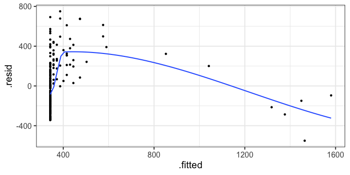<!-- --> --- ```r mod2 = lm(points ~ talent + I(talent^2), data = football) summary(mod2) ``` ``` ## ## Call: ## lm(formula = points ~ talent + I(talent^2), data = football) ## ## Residuals: ## Min 1Q Median 3Q Max ## -384.66 -193.82 -35.34 152.11 729.66 ## ## Coefficients: ## Estimate Std. Error t value Pr(>|t|) ## (Intercept) 305.34402 17.62668 17.323 < 2e-16 *** ## talent 54.89787 5.46864 10.039 < 2e-16 *** ## I(talent^2) -0.57022 0.07499 -7.604 1.01e-12 *** ## --- ## Signif. codes: 0 '***' 0.001 '**' 0.01 '*' 0.05 '.' 0.1 ' ' 1 ## ## Residual standard error: 236.3 on 205 degrees of freedom ## Multiple R-squared: 0.4644, Adjusted R-squared: 0.4592 ## F-statistic: 88.87 on 2 and 205 DF, p-value: < 2.2e-16 ``` --- ```r library(sjPlot) plot_model(mod2, type = "pred") ``` ``` ## $talent ``` 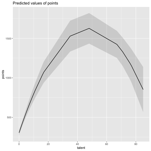<!-- --> --- ## Interpretation The intercept is the predicted value of Y when x = 0 -- this is always the interpretation of the intercept, no matter what kind of regression model you're running. The `\(b_1\)` coefficient is the tangent to the curve when X=0. In other words, this is the rate of change when X is equal to 0. If 0 is not a meaningful value on your X, you may want to center, as this will tell you the rate of change at the mean of X. --- ## Interpretation The `\(b_2\)` coefficient indexes the acceleration, which is how much the slope is going to change. More specifically, `\(2 \times b_2\)` is the acceleration: the rate of change in `\(b_1\)` for a 1-unit change in X. You can use this to calculate the slope of the tangent line at any value of X you're interested in: `$$\large b_1 + (2\times b_2\times X)$$` --- ```r tidy(mod2) ``` ``` ## # A tibble: 3 x 5 ## term estimate std.error statistic p.value ## <chr> <dbl> <dbl> <dbl> <dbl> ## 1 (Intercept) 305. 17.6 17.3 5.22e-42 ## 2 talent 54.9 5.47 10.0 1.53e-19 ## 3 I(talent^2) -0.570 0.0750 -7.60 1.01e-12 ``` .pull-left[ **At X = 10** ```r 54.9 + (2*-.570*10) ``` ``` ## [1] 43.5 ``` ] .pull-right[ **At X = 70** ```r 54.9 + (2*-.570*70) ``` ``` ## [1] -24.9 ``` ] --- ## Polynomials are interactions An term for `\(X^2\)` is a term for `\(X \times X\)` or the multiplication of two independent variables holding the same values. ```r football$talent_2 = football$talent*football$talent tidy(lm(points ~ talent + talent_2, data = football)) ``` ``` ## # A tibble: 3 x 5 ## term estimate std.error statistic p.value ## <chr> <dbl> <dbl> <dbl> <dbl> ## 1 (Intercept) 305. 17.6 17.3 5.22e-42 ## 2 talent 54.9 5.47 10.0 1.53e-19 ## 3 talent_2 -0.570 0.0750 -7.60 1.01e-12 ``` --- ## Polynomials are interactions Put another way: `$$\large \hat{Y} = b_0 + b_1X + b_2X^2$$` `$$\large \hat{Y} = b_0 + \frac{b_1}{2}X + \frac{b_1}{2}X + b_2(X \times X)$$` The interaction term in another model would be interpreted as "how does the slope of X change as I move up in Z?" -- here, we ask "how does the slope of X change as we move up in X?" --- ## When should you use polynomial terms? You may choose to fit a polynomial term after looking at a scatterplot of the data or looking at residual plots. A U-shaped curve may be indicative that you need to fit a quadratic form -- although, as we discussed before, you may actually be measuring a different kind of non-linear relationship. Polynomial terms should mostly be dictated by theory -- if you don't have a good reason for thinking there will be a change in sign, then a polynomial is not right for you. And, of course, if you fit a polynomial regression, be sure to once again check your diagnostics before interpreting the coefficients. --- ```r aug2 = augment(mod2) ggplot(aug2, aes(x = .fitted, y = .resid)) + geom_point() + geom_smooth(se = F) + theme_bw(base_size = 20) ``` 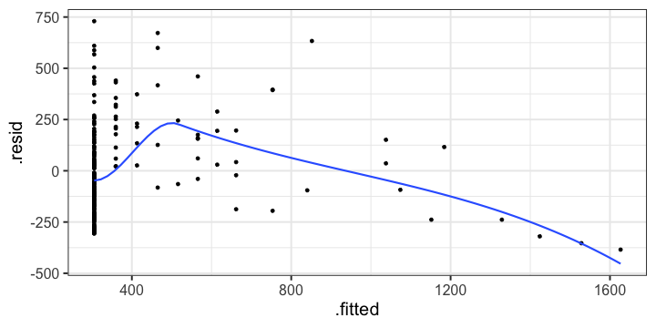<!-- --> --- ```r plot_model(mod2, type = "pred", show.data = T) ``` ``` ## $talent ``` 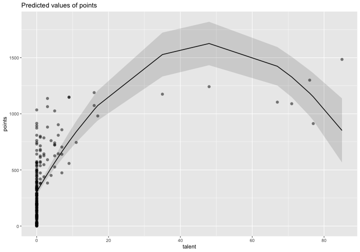<!-- --> --- class: inverse ## Three-way interactions and beyond --- ### Three-way interactions (regression) **Regression equation** `$$\hat{Y} = b_{0} + b_{1}X + b_{2}Z + b_{3}W + b_{4}XZ + b_{5}XW + b_{6}ZW + b_{7}XZW$$` The three-way interaction qualifies the three main effects (and any two-way interactions). Like a two-way interaction, the three-way interaction is a conditional effect. And it is symmetrical, meaning there are several equally correct ways of interpreting it. **Factorial ANOVA** We describe the factorial ANOVA design by the number of levels of each factor. "X by Z by W" (e.g., 2 by 3 by 4, or 2x3x4) --- A two-way (A x B) interaction means that the magnitude of one main effect (e.g., A main effect) depends on levels of the other variable (B). But, it is equally correct to say that the magnitude of the B main effect depends on levels of A. In regression, we refer to these as **conditional effects** and in ANOVA, they are called **simple main effects.** A three-way interaction means that the magnitude of one two-way interaction (e.g., A x B) depends on levels of the remaining variable (C). It is equally correct to say that the magnitude of the A x C interaction depend on levels of B. Or, that the magnitude of the B x C interaction depends on levels of A. These are known as **simple interaction effects**. --- ### Example (regression) ```r psych::describe(stress_data, fast = T) ``` ``` ## Warning in FUN(newX[, i], ...): no non-missing arguments to min; returning Inf ``` ``` ## Warning in FUN(newX[, i], ...): no non-missing arguments to max; returning -Inf ``` ``` ## vars n mean sd min max range se ## gender 1 150 NaN NA Inf -Inf -Inf NA ## bad_day 2 150 2.95 1.29 1 5 4 0.11 ## talk 3 150 2.57 1.20 1 5 4 0.10 ## stress 4 150 30.15 10.00 1 51 50 0.82 ``` ```r table(stress_data$gender) ``` ``` ## ## female male ## 67 83 ``` --- ```r mod_stress = lm(stress ~ bad_day*talk*gender, data = stress_data) summary(mod_stress) ``` ``` ## ## Call: ## lm(formula = stress ~ bad_day * talk * gender, data = stress_data) ## ## Residuals: ## Min 1Q Median 3Q Max ## -10.6126 -3.2974 0.0671 3.1129 10.7774 ## ## Coefficients: ## Estimate Std. Error t value Pr(>|t|) ## (Intercept) 20.3385 4.5181 4.502 1.39e-05 *** ## bad_day 2.5273 1.6596 1.523 0.13003 ## talk 2.4870 1.3234 1.879 0.06227 . ## gendermale -0.1035 5.7548 -0.018 0.98568 ## bad_day:talk -1.4220 0.4564 -3.116 0.00222 ** ## bad_day:gendermale -0.1244 2.0069 -0.062 0.95067 ## talk:gendermale 1.9797 2.2823 0.867 0.38718 ## bad_day:talk:gendermale 1.5260 0.7336 2.080 0.03931 * ## --- ## Signif. codes: 0 '***' 0.001 '**' 0.01 '*' 0.05 '.' 0.1 ' ' 1 ## ## Residual standard error: 4.733 on 142 degrees of freedom ## Multiple R-squared: 0.7865, Adjusted R-squared: 0.776 ## F-statistic: 74.72 on 7 and 142 DF, p-value: < 2.2e-16 ``` --- ```r library(reghelper) simple_slopes(mod_stress) ``` ``` ## bad_day talk gender Test Estimate Std. Error t value df Pr(>|t|) Sig. ## 1 1.661455 1.365903 sstest 5.8571 1.7437 3.3590 142 0.0010045 ** ## 2 2.953333 1.365903 sstest 8.3892 1.5671 5.3535 142 3.386e-07 *** ## 3 4.245211 1.365903 sstest 10.9214 2.5606 4.2651 142 3.627e-05 *** ## 4 1.661455 2.566667 sstest 11.2788 1.4571 7.7406 142 1.687e-12 *** ## 5 2.953333 2.566667 sstest 16.1781 1.0985 14.7274 142 < 2.2e-16 *** ## 6 4.245211 2.566667 sstest 21.0775 1.6775 12.5647 142 < 2.2e-16 *** ## 7 1.661455 3.767431 sstest 16.7004 2.3888 6.9912 142 9.806e-11 *** ## 8 2.953333 3.767431 sstest 23.9670 1.4830 16.1608 142 < 2.2e-16 *** ## 9 4.245211 3.767431 sstest 31.2335 2.0578 15.1784 142 < 2.2e-16 *** ## 10 1.661455 sstest female 0.1245 0.7221 0.1724 142 0.8633621 ## 11 2.953333 sstest female -1.7125 0.5996 -2.8558 142 0.0049366 ** ## 12 4.245211 sstest female -3.5495 0.9450 -3.7561 142 0.0002511 *** ## 13 sstest 1.365903 female 0.5850 1.0725 0.5455 142 0.5862803 ## 14 sstest 2.566667 female -1.1224 0.6181 -1.8160 142 0.0714796 . ## 15 sstest 3.767431 female -2.8299 0.4630 -6.1115 142 9.006e-09 *** ## 16 1.661455 sstest male 4.6396 1.0195 4.5510 142 1.137e-05 *** ## 17 2.953333 sstest male 4.7741 0.6463 7.3862 142 1.177e-11 *** ## 18 4.245211 sstest male 4.9085 0.9474 5.1813 142 7.418e-07 *** ## 19 sstest 1.365903 male 2.5451 0.5036 5.0533 142 1.315e-06 *** ## 20 sstest 2.566667 male 2.6700 0.6116 4.3655 142 2.427e-05 *** ## 21 sstest 3.767431 male 2.7950 1.2025 2.3244 142 0.0215233 * ``` --- ```r plot_model(mod_stress, type = "int", mdrt.values = "meansd") ``` <!-- --> --- As a reminder, centering will change all but the highest-order terms in a model. ```r stress_data = stress_data %>% mutate(bad_day_c = bad_day - mean(bad_day), talk_c = talk - mean(talk)) newmod = lm(stress ~ bad_day_c*talk_c*gender, data = stress_data) ``` --- ```r tidy(mod_stress) ``` ``` ## # A tibble: 8 x 5 ## term estimate std.error statistic p.value ## <chr> <dbl> <dbl> <dbl> <dbl> ## 1 (Intercept) 20.3 4.52 4.50 0.0000139 ## 2 bad_day 2.53 1.66 1.52 0.130 ## 3 talk 2.49 1.32 1.88 0.0623 ## 4 gendermale -0.104 5.75 -0.0180 0.986 ## 5 bad_day:talk -1.42 0.456 -3.12 0.00222 ## 6 bad_day:gendermale -0.124 2.01 -0.0620 0.951 ## 7 talk:gendermale 1.98 2.28 0.867 0.387 ## 8 bad_day:talk:gendermale 1.53 0.734 2.08 0.0393 ``` ```r tidy(newmod) ``` ``` ## # A tibble: 8 x 5 ## term estimate std.error statistic p.value ## <chr> <dbl> <dbl> <dbl> <dbl> ## 1 (Intercept) 23.4 0.845 27.7 3.89e-59 ## 2 bad_day_c -1.12 0.618 -1.82 7.15e- 2 ## 3 talk_c -1.71 0.600 -2.86 4.94e- 3 ## 4 gendermale 16.2 1.10 14.7 2.20e-30 ## 5 bad_day_c:talk_c -1.42 0.456 -3.12 2.22e- 3 ## 6 bad_day_c:gendermale 3.79 0.870 4.36 2.47e- 5 ## 7 talk_c:gendermale 6.49 0.882 7.36 1.38e-11 ## 8 bad_day_c:talk_c:gendermale 1.53 0.734 2.08 3.93e- 2 ``` --- ### Four-way? $$ `\begin{aligned} \hat{Y} &= b_0 + b_1X + b_{2}Z + b_{3}W + b_{4}Q + b_{5}XW\\ &+ b_{6}ZW + b_{7}XZ + b_{8}QX + b_{9}QZ + b_{10}QW\\ &+ b_{11}XZQ + b_{12}XZW + b_{13}XWQ + b_{14}ZWQ + b_{15}XZWQ\\ \end{aligned}` $$ -- 3-way (and higher) interactions are incredibly difficult to interpret, in part because they represent incredibly complicated processes. If you have a solid theoretical rationale for conducting a 3-day interaction, be sure you've collected enough subjects to power your test (more on this later). --- Especially with small samples, three-way interactions may be the result of a few outliers skewing a regression line. If you have stumbled upon a three-way interactoin during exploratory analyses, **be careful.** This is far more likely to be a result of over-fitting than uncovering a true underlying process. Best practice for 3-way (and higher) interactions is to use at least one nominal moderator (ideally with only 2 levels), instead of all continuous moderators. This allows you to examine the 2-way interaction at each level of the nominal moderator. Even better if one of these moderators is experimenter manipulated, which increases the likelihood of balanced conditions. --- class: inverse no more interactions --- ## Homoscedasticity Homoscedasticity is the assumption that the variance of Y is constant across all levels of a predictor. ```r library(tidyverse) ggplot(Data, aes(x = calm, y = problems)) + geom_point(alpha = .5, position = position_jitter(width = 0, height = .1)) ``` <!-- --> --- ## Weighted least squares Weighted least squares (WLS) is a commonly used remedial procedure for heteroscedasticity (or failiing to meet the assumptino of homoscedasticity). In an ordinary least squares (OLS) approach, each case in the dataset is given equal weight. WLS assigns each case a weight `\(w_i\)`, depending upon the precision of the observation of Y in that case. For observations for which the variance around the residuals around the regression line is low, the case is given a high weight. --- Recall that an OLS estimation chooses values of `\(b_0\)` and `\(b_1\)` that minimizes the sum of squared residuals: `$$\large \text{min}(\sum e^2_i) = \text{min} \sum (Y_i-b_1X_i-b_0)^2$$` In a WLS approach, weights are taken into account, such that the values of `\(b_0\)` and `\(b_1\)` are chosen to minimize the sum of the **weighted** squared residuals: `$$\large \text{min}(\sum w_ie^2_i) = \text{min} \sum w_i(Y_i-b_1X_i-b_0)^2$$` The value of the weights is the inverse of the conditional variance of the residuals in the population corresponding to the specified value of X: `$$\large w_i = \frac{1}{\sigma^2_{Y-\hat{Y}|X}}$$` --- The value of `\(\sigma^2_{Y-\hat{Y}|X}\)`, the variance of the residuals in the population conditional on X, is not known and must be estimated. A common procedure for estimating weights is to estimate the usual OLS regression equation, square the residuals, and then regress the squared residuals onto X. The weight is then estimated as the inverse of the predicted value for a case. Using our own data: ```r ols.model = lm(problems ~ calm, data = Data) library(broom) ols_aug = augment(ols.model) head(ols_aug) ``` ``` ## # A tibble: 6 x 9 ## problems calm .fitted .se.fit .resid .hat .sigma .cooksd .std.resid ## <dbl> <dbl> <dbl> <dbl> <dbl> <dbl> <dbl> <dbl> <dbl> ## 1 4 1.06 4.87 0.121 -0.872 0.0326 0.665 0.0296 -1.33 ## 2 5 1.24 4.70 0.111 0.304 0.0278 0.671 0.00306 0.462 ## 3 6 1.30 4.63 0.108 1.37 0.0263 0.653 0.0581 2.07 ## 4 4 0.852 5.08 0.132 -1.08 0.0391 0.660 0.0558 -1.66 ## 5 5 1.12 4.82 0.118 0.180 0.0311 0.672 0.00120 0.273 ## 6 5 0.715 5.22 0.140 -0.223 0.0438 0.672 0.00266 -0.341 ``` --- ```r # square residuals ols_aug$resid_sq = ols_aug$.resid^2 # regress squared resid on predictor weight.mod = lm(resid_sq ~ calm, data = ols_aug) ``` .pull-left[ ```r coef(ols.model) ``` ``` ## (Intercept) calm ## 5.941940 -1.005699 ``` ] .pull-right[ ```r coef(weight.mod) ``` ``` ## (Intercept) calm ## 1.0739505 -0.2591579 ``` ] ```r # extract predicted values pred.resid = predict(weight.mod) head(pred.resid) ``` ``` ## 1 2 3 4 5 6 ## 0.7982546 0.7527584 0.7366885 0.8530291 0.7849316 0.8886457 ``` ```r # find inverse of predicted values # use absolute value if some of your predicted values are negative est.weights = 1/abs(pred.resid) head(est.weights) ``` ``` ## 1 2 3 4 5 6 ## 1.252733 1.328447 1.357426 1.172293 1.273996 1.125308 ``` --- ```r wls.model = lm(problems ~ calm, data = Data, weights = est.weights) ``` #### OLS solution ```r tidy(ols.model) ``` ``` ## # A tibble: 2 x 5 ## term estimate std.error statistic p.value ## <chr> <dbl> <dbl> <dbl> <dbl> ## 1 (Intercept) 5.94 0.182 32.6 3.54e-47 ## 2 calm -1.01 0.0675 -14.9 1.58e-24 ``` #### WLS solution ```r tidy(wls.model) ``` ``` ## # A tibble: 2 x 5 ## term estimate std.error statistic p.value ## <chr> <dbl> <dbl> <dbl> <dbl> ## 1 (Intercept) 5.64 0.182 30.9 1.60e-45 ## 2 calm -0.884 0.0451 -19.6 7.58e-32 ``` --- <!-- --> --- WLS is a robust method for dealing with heteroscedasticity. What if you violate the normality assumption of regression? -- A **bootstrapping** approach is useful when the theoretical sampling distribution for an estimate is unknown or unverifiable. In other words, if you have reason to suspect that either the variables in your model are not normally distributed, or that they're non-normally distributed, then bootstrapping can help ensure non-bias estimation and appropriately sized confidence intervals. --- ## Bootstrapping In bootstrapping, the theoretical sampling distribution is assumed to be unknown or unverifiable. Under the weak assumption that the sample in hand is representative of some population, then that population sampling distribution can be built empirically by randomly sampling with replacement from the sample. The resulting empirical sampling distribution can be used to construct confidence intervals and make inferences. --- ### Illustration Imagine you had a sample of 6 people: Rachel, Monica, Phoebe, Joey, Chandler, and Ross. To bootstrap their heights, you would draw from this group many samples of 6 people *with replacement*, each time calculating the average height of the sample. ``` ## [1] "Chandler" "Ross" "Phoebe" "Monica" "Rachel" "Monica" ``` ``` ## [1] 68 ``` ``` ## [1] "Rachel" "Ross" "Rachel" "Chandler" "Ross" "Monica" ``` ``` ## [1] 68.83333 ``` ``` ## [1] "Rachel" "Chandler" "Chandler" "Phoebe" "Monica" "Monica" ``` ``` ## [1] 67.83333 ``` ``` ## [1] "Phoebe" "Phoebe" "Ross" "Joey" "Phoebe" "Phoebe" ``` ``` ## [1] 69.16667 ``` ``` ## [1] "Chandler" "Ross" "Ross" "Joey" "Rachel" "Chandler" ``` ``` ## [1] 70.83333 ``` ``` ## [1] "Rachel" "Chandler" "Ross" "Chandler" "Rachel" "Joey" ``` ``` ## [1] 69.5 ``` ``` ## [1] "Phoebe" "Rachel" "Chandler" "Ross" "Monica" "Joey" ``` ``` ## [1] 68.83333 ``` ``` ## [1] "Ross" "Chandler" "Phoebe" "Chandler" "Rachel" "Rachel" ``` ``` ## [1] 69.16667 ``` ??? ```r heights ``` ``` ## Rachel Monica Phoebe Joey Chandler Ross ## 65 65 68 70 72 73 ``` --- ### Illustration ```r boot = 10000 friends = c("Rachel", "Monica", "Phoebe", "Joey", "Chandler", "Ross") heights = c(65, 65, 68, 70, 72, 73) sample_means = numeric(length = boot) for(i in 1:boot){ this_sample = sample(heights, size = length(heights), replace = T) sample_means[i] = mean(this_sample) } ``` --- ## Illustration <!-- --> --- ### Example A sample of 216 response times. What is their central tendency and variability? There are several candidates for central tendency (e.g., mean, median) and for variability (e.g., standard deviation, interquartile range). Some of these do not have well understood theoretical sampling distributions. For the mean and standard deviation, we have theoretical sampling distributions to help us, provided we think the mean and standard deviation are the best indices. For the others, we can use bootstrapping. --- 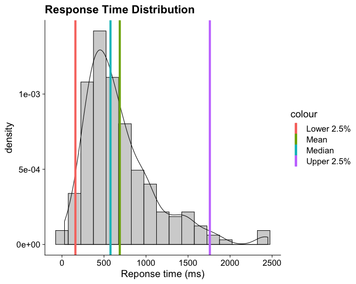<!-- --> --- ### Bootstrapping Before now, if we wanted to estimate the mean and the 95% confidence interval around the mean, we would find the theoretical sampling distribution by scaling a t-distribution to be centered on the mean of our sample and have a standard deviation equal to `\(\frac{s}{\sqrt{N}}.\)` But we have to make many assumptions to use this sampling distribution, and we may have good reason not to. Instead, we can build a population sampling distribution empirically by randomly sampling with replacement from the sample. --- ## Response time example ```r boot = 10000 response_means = numeric(length = boot) for(i in 1:boot){ sample_response = sample(response, size = 216, replace = T) response_means[i] = mean(sample_response) } ``` 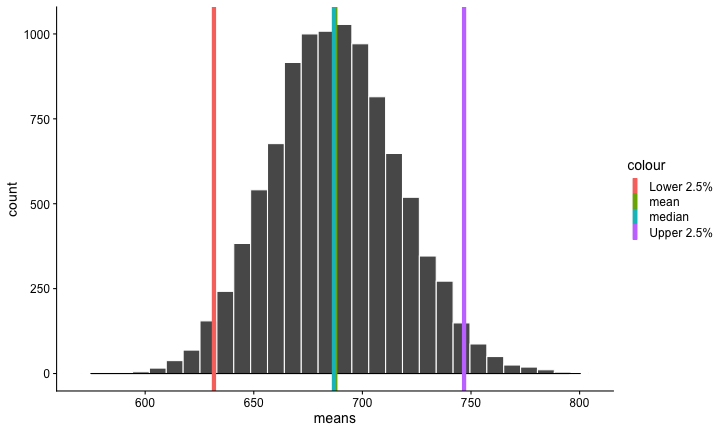<!-- --> --- ```r mean(response_means) ``` ``` ## [1] 687.5221 ``` ```r median(response_means) ``` ``` ## [1] 686.9085 ``` ```r quantile(response_means, probs = c(.025, .975)) ``` ``` ## 2.5% 97.5% ## 631.6661 746.8103 ``` What about something like the median? --- ```r boot = 10000 response_med = numeric(length = boot) for(i in 1:boot){ sample_response = sample(response, size = 216, replace = T) response_med[i] = median(sample_response) } ``` .pull-left[ 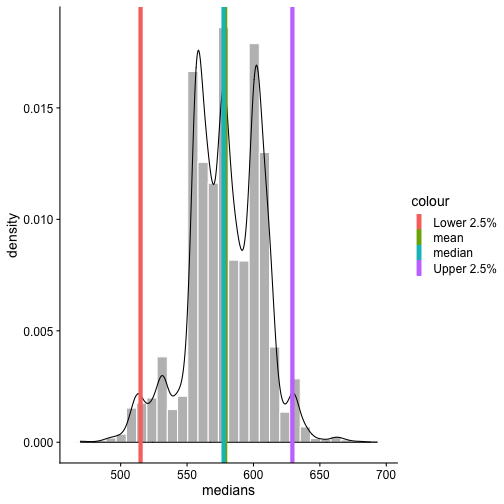<!-- --> ] .pull-right[ ```r mean(response_med) ``` ``` ## [1] 578.6673 ``` ```r median(response_med) ``` ``` ## [1] 577.5063 ``` ```r quantile(response_med, probs = c(.025, .975)) ``` ``` ## 2.5% 97.5% ## 514.9828 629.3005 ``` ] --- ```r boot = 10000 response_sd = numeric(length = boot) for(i in 1:boot){ sample_response = sample(response, size = 216, replace = T) response_sd[i] = sd(sample_response) } ``` .pull-left[ 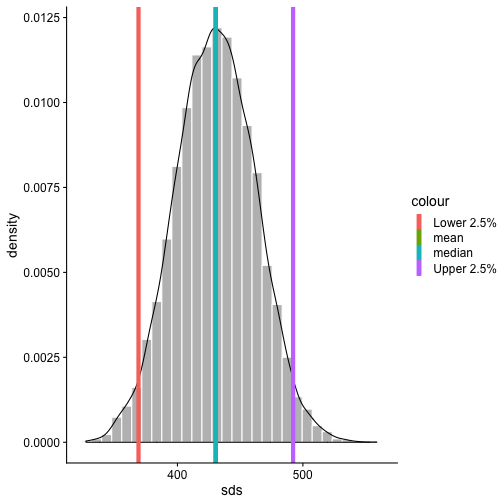<!-- --> ] .pull-right[ ```r mean(response_sd) ``` ``` ## [1] 430.5541 ``` ```r median(response_sd) ``` ``` ## [1] 430.3614 ``` ```r quantile(response_sd, probs = c(.025, .975)) ``` ``` ## 2.5% 97.5% ## 368.9656 492.1912 ``` ] --- class: inverse ## Next time... Finish bootstrapping Yarkoni and Westfall (2017) and the lessons of machine learning