class: center, middle, inverse, title-slide # Bootstrapping --- #Last time... - Polynomials - 3-way interactions - Weighted least squares # Today * Boostrapping * Lessons from machine learning --- ## Bootstrapping In bootstrapping, the theoretical sampling distribution is assumed to be unknown or unverifiable. Under the weak assumption that the sample in hand is representative of some population, then that population sampling distribution can be built empirically by randomly sampling with replacement from the sample. The resulting empirical sampling distribution can be used to construct confidence intervals and make inferences. --- ### Illustration Imagine you had a sample of 6 people: Rachel, Monica, Phoebe, Joey, Chandler, and Ross. To bootstrap their heights, you would draw from this group many samples of 6 people *with replacement*, each time calculating the average height of the sample. ``` ## [1] "Ross" "Monica" "Joey" "Monica" "Joey" "Monica" ``` ``` ## [1] 68 ``` ``` ## [1] "Phoebe" "Rachel" "Rachel" "Ross" "Monica" "Ross" ``` ``` ## [1] 68.16667 ``` ``` ## [1] "Monica" "Joey" "Monica" "Joey" "Joey" "Joey" ``` ``` ## [1] 68.33333 ``` ``` ## [1] "Rachel" "Phoebe" "Monica" "Phoebe" "Rachel" "Joey" ``` ``` ## [1] 66.83333 ``` ``` ## [1] "Phoebe" "Rachel" "Monica" "Ross" "Rachel" "Joey" ``` ``` ## [1] 67.66667 ``` ``` ## [1] "Joey" "Joey" "Monica" "Ross" "Chandler" "Phoebe" ``` ``` ## [1] 69.66667 ``` ``` ## [1] "Chandler" "Ross" "Joey" "Rachel" "Monica" "Joey" ``` ``` ## [1] 69.16667 ``` ``` ## [1] "Rachel" "Phoebe" "Joey" "Chandler" "Monica" "Ross" ``` ``` ## [1] 68.83333 ``` ??? ```r heights ``` ``` ## Rachel Monica Phoebe Joey Chandler Ross ## 65 65 68 70 72 73 ``` --- ### Illustration ```r boot = 10000 friends = c("Rachel", "Monica", "Phoebe", "Joey", "Chandler", "Ross") heights = c(65, 65, 68, 70, 72, 73) sample_means = numeric(length = boot) for(i in 1:boot){ this_sample = sample(heights, size = length(heights), replace = T) sample_means[i] = mean(this_sample) } ``` --- ## Illustration 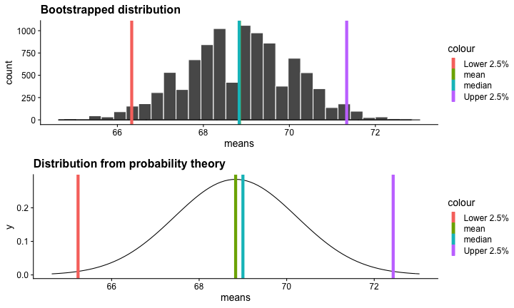<!-- --> --- ### Example A sample of 216 response times. What is their central tendency and variability? There are several candidates for central tendency (e.g., mean, median) and for variability (e.g., standard deviation, interquartile range). Some of these do not have well understood theoretical sampling distributions. For the mean and standard deviation, we have theoretical sampling distributions to help us, provided we think the mean and standard deviation are the best indices. For the others, we can use bootstrapping. --- 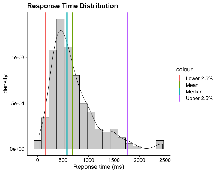<!-- --> --- ### Bootstrapping Before now, if we wanted to estimate the mean and the 95% confidence interval around the mean, we would find the theoretical sampling distribution by scaling a t-distribution to be centered on the mean of our sample and have a standard deviation equal to `\(\frac{s}{\sqrt{N}}.\)` But we have to make many assumptions to use this sampling distribution, and we may have good reason not to. Instead, we can build a population sampling distribution empirically by randomly sampling with replacement from the sample. --- ## Response time example ```r boot = 10000 response_means = numeric(length = boot) for(i in 1:boot){ sample_response = sample(response, size = 216, replace = T) response_means[i] = mean(sample_response) } ``` 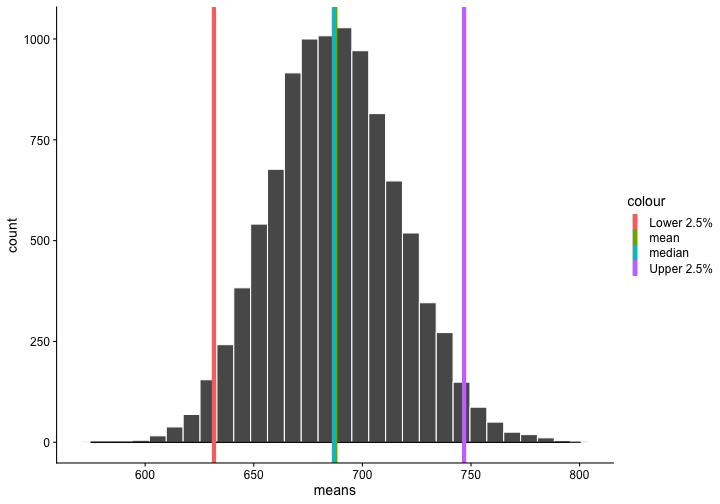<!-- --> --- ```r mean(response_means) ``` ``` ## [1] 687.5221 ``` ```r median(response_means) ``` ``` ## [1] 686.9085 ``` ```r quantile(response_means, probs = c(.025, .975)) ``` ``` ## 2.5% 97.5% ## 631.6661 746.8103 ``` What about something like the median? --- ### bootstrapped distribution of the median ```r boot = 10000 response_med = numeric(length = boot) for(i in 1:boot){ sample_response = sample(response, size = 216, replace = T) response_med[i] = median(sample_response) } ``` .pull-left[ 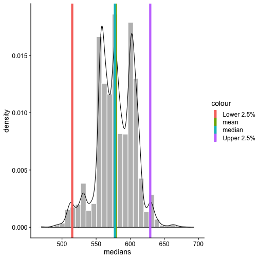<!-- --> ] .pull-right[ ```r mean(response_med) ``` ``` ## [1] 578.6673 ``` ```r median(response_med) ``` ``` ## [1] 577.5063 ``` ```r quantile(response_med, probs = c(.025, .975)) ``` ``` ## 2.5% 97.5% ## 514.9828 629.3005 ``` ] --- ### bootstrapped distribution of the standard deviation ```r boot = 10000 response_sd = numeric(length = boot) for(i in 1:boot){ sample_response = sample(response, size = 216, replace = T) response_sd[i] = sd(sample_response) } ``` .pull-left[ 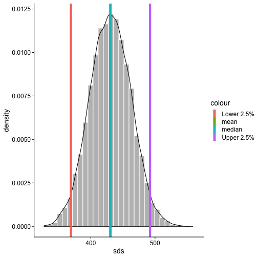<!-- --> ] .pull-right[ ```r mean(response_sd) ``` ``` ## [1] 430.5541 ``` ```r median(response_sd) ``` ``` ## [1] 430.3614 ``` ```r quantile(response_sd, probs = c(.025, .975)) ``` ``` ## 2.5% 97.5% ## 368.9656 492.1912 ``` ] --- You can bootstrap estimates and 95% confidence intervals for *any* statistics you'll need to estimate. The `boot` function provides some functions to speed this process along. ```r library(boot) # function to obtain R-Squared from the data rsq <- function(data, indices) { d <- data[indices,] # allows boot to select sample fit <- lm(mpg~wt+disp, data=d) # this is the code you would have run return(summary(fit)$r.square) } # bootstrapping with 10000 replications results <- boot(data=mtcars, statistic=rsq, R=10000) ``` --- .pull-left[ ```r data.frame(rsq = results$t) %>% ggplot(aes(x = rsq)) + geom_histogram(color = "white", bins = 30) ``` 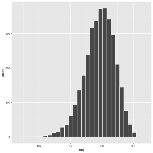<!-- --> ] .pull-right[ ```r median(results$t) ``` ``` ## [1] 0.7962501 ``` ```r boot.ci(results, type = "perc") ``` ``` ## BOOTSTRAP CONFIDENCE INTERVAL CALCULATIONS ## Based on 10000 bootstrap replicates ## ## CALL : ## boot.ci(boot.out = results, type = "perc") ## ## Intervals : ## Level Percentile ## 95% ( 0.6871, 0.8773 ) ## Calculations and Intervals on Original Scale ``` ] --- ### Example 2 Samples of service waiting times for Verizon’s (ILEC) versus other carriers (CLEC) customers. In this district, Verizon must provide line service to all customers or else face a fine. The question is whether the non-Verizon customers are getting ignored or facing greater variability in waiting times. ```r Verizon = read.csv(here("data/Verizon.csv")) ``` 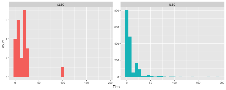<!-- --> --- 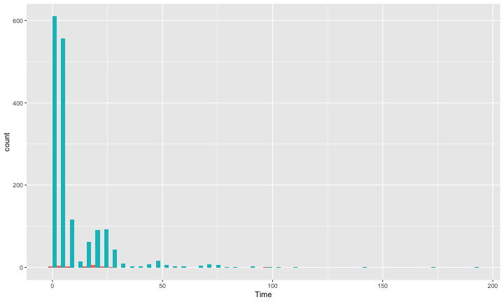<!-- --> ``` ## ## CLEC ILEC ## 23 1664 ``` --- There's no world in which these data meet the typical assumptions of an independent samples t-test. To estimate mean differences we can use boostrapping. Here, we'll resample with replacement separately from the two samples. ```r boot = 10000 difference = numeric(length = boot) subsample_CLEC = Verizon %>% filter(Group == "CLEC") subsample_ILEC = Verizon %>% filter(Group == "ILEC") for(i in 1:boot){ sample_CLEC = sample(subsample_CLEC$Time, size = nrow(subsample_CLEC), replace = T) sample_ILEC = sample(subsample_ILEC$Time, size = nrow(subsample_ILEC), replace = T) difference[i] = mean(sample_CLEC) - mean(sample_ILEC) } ``` --- <!-- --> The difference in means is 7.62 `\([1.64,16.72]\)`. --- ### Bootstrapping Summary Bootstrapping can be a useful tool to estimate parameters when 1. you've violated assumptions of the test (i.e., normality, homoskedasticity) 2. you have good reason to believe the sampling distribution is not normal, but don't know what it is 3. there are other oddities in your data, like very unbalanced samples This allows you to create a confidence interval around any statistic you want -- Cronbach's alpha, ICC, Mahalanobis Distance, `\(R^2\)`, AUC, etc. * You can test whether these statistics are significantly different from any other value -- how? --- ### Bootstrapping Summary Bootstrapping will NOT help you deal with: * dependence between observations -- for this, you'll need to explicity model dependence (e.g., multilevel model, repeated measures ANOVA) * improperly specified models or forms -- use theory to guide you here * measurement error -- why bother? --- ## Yarkoni and Westfall (2017) Y&W describe the goals of explanation and prediction in science; how are these goals similar to each other and how are they in opposition to each other? According to Y&W, how should psychologists change their research, in terms of explanation and prediction, and why? How do regression models fit into the goals of explanation and prediction? Where do they fall short on one or other or both? ??? Explanation: describe causal underpinnings of behaviors/outcomes Prediction: accurately forecast behaviors/outcomes Similar: both goals of science; good prediction can help us develop theory of explanation and vice versa Statistical tension with one another: statistical models that accurately describe causal truths often have poor prediction and are complex; predictive models are often very different from the data-generating processes. Y&W: we should spend more time and resources developing predictive models than we do not (not necessarily than explanation models, although they probably think that's true) --- ## Yarkoni and Westfall (2017) What is **overfitting** and where does this occur in terms of the models we have discussed in class thus far? What is **bias** and **variance**, and how does the bias-variance trade-off relate to overfitting? * How concerned are you about overfitting in your own area of research? How about in the studies you'd like to do in the next couple of years? ??? Overfitting: mistakenly fitting sample-specific noise as if it were signal OLS models tend to be overfit because they minimize error for a specific sample Bias: systematically over or under estimating parameters Variance: how much estimates tend to jump around Model-fits tend to prioritizie minimizing bias or variance, and choosing to minimize one inflates the other; OLS models minimize one of these --- ## Yarkoni and Westfall (2017) How do Y&W propose adjusting our current statistical practices to be more successful at prediction? ??? big data sets Cross-validation regularization --- ## Yarkoni and Westfall (2017) **Big Data** * Reduce the likelihood of overfitting -- more data means less error **Cross-validation** * Is my model overfit? **Regularization** * Constrain the model to be less overfit --- ### Big Data Sets "Every pattern that could be observed in a given dataset reflects some... unknown combination of signal and error" (page 1104). Error is random, so it cannot correlate with anything; as we aggregate many pieces of information together, we reduce error. Thus, as we get bigger and bigger datasets, the amount of error we have gets smaller and smaller --- ### Cross-validation **Cross-validation** is a family of techniques that involve testing and training a model on different samples of data. * Replication * Hold-out samples * K-fold * Split the original dataset into 2(+) datasets, train a model on one set, test it in the other * Recycle: each dataset can be a training AND a testing; average model fit results to get better estimate of fit * Can split the dataset into more than 2 sections --- ```r library(here) stress.data = read.csv(here("data/stress.csv")) library(psych) describe(stress.data, fast = T) ``` ``` ## vars n mean sd min max range se ## id 1 118 488.65 295.95 2.00 986.00 984.00 27.24 ## Anxiety 2 118 7.61 2.49 0.70 14.64 13.94 0.23 ## Stress 3 118 5.18 1.88 0.62 10.32 9.71 0.17 ## Support 4 118 8.73 3.28 0.02 17.34 17.32 0.30 ## group 5 118 NaN NA Inf -Inf -Inf NA ``` ```r model.lm = lm(Stress ~ Anxiety*Support*group, data = stress.data) summary(model.lm)$r.squared ``` ``` ## [1] 0.4126943 ``` --- ### Example: 10-fold cross validation ```r # new package! library(caret) # set control parameters ctrl <- trainControl(method="cv", number=10) # use train() instead of lm() cv.model <- train(Stress ~ Anxiety*Support*group, data = stress.data, trControl=ctrl, # what are the control parameters method="lm") # what kind of model cv.model ``` ``` ## Linear Regression ## ## 118 samples ## 3 predictor ## ## No pre-processing ## Resampling: Cross-Validated (10 fold) ## Summary of sample sizes: 106, 106, 106, 106, 107, 106, ... ## Resampling results: ## ## RMSE Rsquared MAE ## 1.541841 0.3438326 1.237663 ## ## Tuning parameter 'intercept' was held constant at a value of TRUE ``` --- ### Regularization Penalizing a model as it grows more complex. * Usually involves shrinking coefficient estimates -- the model will fit less well in-sample but may be more predictive *lasso regression*: balance minimizing sum of squared residuals (OLS) and minimizing smallest sum of absolute values of coefficients - coefficients are more biased (tend to underestimate coefficients) but produce less variability in results The coefficient `\(\lambda\)` is used to penalize the model. --- The `glmnet` package has the tools for lasso regression. One small complication is that the package uses matrix algebra, so you need to feed it a matrix of predictors -- specifically, instead of saying "find the interaction between A and B", you need to create the variable that represents this term. How could you do that manually? -- Luckily, the function `model.matrix()` can do this for you. --- ```r # provide your original lm model to get matrix of predictors X.matrix <- model.matrix.lm(model.lm) head(X.matrix) ``` ``` ## (Intercept) Anxiety Support groupTx Anxiety:Support Anxiety:groupTx ## 1 1 10.18520 6.1602 1 62.74287 10.1852 ## 2 1 5.58873 8.9069 0 49.77826 0.0000 ## 3 1 6.58500 10.5433 1 69.42763 6.5850 ## 4 1 8.95430 11.4605 1 102.62076 8.9543 ## 5 1 7.59910 5.5516 0 42.18716 0.0000 ## 6 1 8.15600 7.5117 1 61.26543 8.1560 ## Support:groupTx Anxiety:Support:groupTx ## 1 6.1602 62.74287 ## 2 0.0000 0.00000 ## 3 10.5433 69.42763 ## 4 11.4605 102.62076 ## 5 0.0000 0.00000 ## 6 7.5117 61.26543 ``` ```r library(glmnet) lasso.mod <- glmnet(x = X.matrix[,-1], #don't need the intercept y = stress.data$Stress) ``` --- ```r lasso.mod ``` ``` ## ## Call: glmnet(x = X.matrix[, -1], y = stress.data$Stress) ## ## Df %Dev Lambda ## 1 0 0.00000 0.97920 ## 2 1 0.04664 0.89220 ## 3 1 0.08537 0.81300 ## 4 1 0.11750 0.74080 ## 5 1 0.14420 0.67500 ## 6 1 0.16640 0.61500 ## 7 1 0.18480 0.56040 ## 8 1 0.20000 0.51060 ## 9 1 0.21270 0.46520 ## 10 1 0.22320 0.42390 ## 11 1 0.23200 0.38620 ## 12 2 0.24110 0.35190 ## 13 2 0.24980 0.32070 ## 14 2 0.25700 0.29220 ## 15 2 0.26290 0.26620 ## 16 3 0.27400 0.24260 ## 17 2 0.29390 0.22100 ## 18 2 0.30440 0.20140 ## 19 2 0.31310 0.18350 ## 20 2 0.32030 0.16720 ## 21 2 0.32630 0.15230 ## 22 2 0.33130 0.13880 ## 23 2 0.33540 0.12650 ## 24 2 0.33880 0.11520 ## 25 2 0.34170 0.10500 ## 26 2 0.34410 0.09567 ## 27 2 0.34600 0.08717 ## 28 2 0.34760 0.07943 ## 29 2 0.34900 0.07237 ## 30 3 0.35400 0.06594 ## 31 3 0.36320 0.06009 ## 32 3 0.37090 0.05475 ## 33 3 0.37720 0.04988 ## 34 3 0.38250 0.04545 ## 35 3 0.38690 0.04141 ## 36 4 0.39060 0.03774 ## 37 4 0.39350 0.03438 ## 38 4 0.39610 0.03133 ## 39 4 0.39810 0.02855 ## 40 4 0.39990 0.02601 ## 41 4 0.40130 0.02370 ## 42 4 0.40250 0.02159 ## 43 4 0.40350 0.01968 ## 44 6 0.40450 0.01793 ## 45 5 0.40570 0.01633 ## 46 5 0.40650 0.01488 ## 47 5 0.40720 0.01356 ## 48 5 0.40780 0.01236 ## 49 5 0.40830 0.01126 ## 50 6 0.40880 0.01026 ## 51 6 0.40950 0.00935 ## 52 6 0.41000 0.00852 ## 53 6 0.41040 0.00776 ## 54 6 0.41080 0.00707 ## 55 6 0.41110 0.00644 ## 56 6 0.41130 0.00587 ## 57 6 0.41150 0.00535 ## 58 6 0.41170 0.00487 ## 59 6 0.41180 0.00444 ## 60 6 0.41190 0.00405 ## 61 6 0.41200 0.00369 ## 62 6 0.41210 0.00336 ## 63 6 0.41220 0.00306 ## 64 6 0.41220 0.00279 ## 65 6 0.41230 0.00254 ## 66 6 0.41230 0.00231 ## 67 6 0.41240 0.00211 ## 68 7 0.41240 0.00192 ## 69 7 0.41240 0.00175 ## 70 7 0.41240 0.00160 ## 71 7 0.41250 0.00145 ## 72 7 0.41250 0.00132 ## 73 7 0.41250 0.00121 ## 74 7 0.41250 0.00110 ## 75 7 0.41250 0.00100 ## 76 7 0.41260 0.00091 ## 77 7 0.41260 0.00083 ## 78 7 0.41260 0.00076 ## 79 7 0.41260 0.00069 ## 80 7 0.41260 0.00063 ## 81 7 0.41260 0.00057 ## 82 7 0.41260 0.00052 ## 83 7 0.41260 0.00048 ## 84 7 0.41260 0.00043 ## 85 7 0.41260 0.00040 ## 86 7 0.41260 0.00036 ## 87 7 0.41260 0.00033 ``` ??? DF = number of non-zero coefficients dev = `\(R^2\)` lambda = complexity parameter (how much to downweight, between 0 and 1) --- ### What value of `\(\lambda\)` to choose? ```r plot(lasso.mod, xvar = "dev", label = T) ``` <!-- --> Looks like coefficients 1, 2, and 3 have high values even with shrinkage. --- ### What value of `\(\lambda\)` to choose? ```r plot(lasso.mod, xvar = "lambda", label = TRUE) ``` <!-- --> I might look for lambda values where those coefficients are still different from 0. --- .pull-left[ ```r coef = coef(lasso.mod, s = exp(-5)) coef ``` ``` ## 8 x 1 sparse Matrix of class "dgCMatrix" ## 1 ## (Intercept) -2.211802705 ## Anxiety 0.572946040 ## Support 0.621714623 ## groupTx -0.487719327 ## Anxiety:Support -0.038680253 ## Anxiety:groupTx . ## Support:groupTx 0.029353883 ## Anxiety:Support:groupTx 0.003006013 ``` ] .pull-left[ ```r coef = coef(lasso.mod, s = exp(-4)) coef ``` ``` ## 8 x 1 sparse Matrix of class "dgCMatrix" ## 1 ## (Intercept) -1.8538689387 ## Anxiety 0.5028481785 ## Support 0.5837254774 ## groupTx -0.0044703271 ## Anxiety:Support -0.0302949960 ## Anxiety:groupTx -0.0034894821 ## Support:groupTx 0.0009984811 ## Anxiety:Support:groupTx . ``` ] --- ```r coef = coef(lasso.mod, s = 0) coef ``` ``` ## 8 x 1 sparse Matrix of class "dgCMatrix" ## 1 ## (Intercept) -2.373766131 ## Anxiety 0.612812455 ## Support 0.650290859 ## groupTx -1.044285344 ## Anxiety:Support -0.045146588 ## Anxiety:groupTx 0.025299852 ## Support:groupTx 0.048852216 ## Anxiety:Support:groupTx 0.005913829 ``` `\(\lambda = 0\)` is pretty close to our OLS solution --- ```r coef = coef(lasso.mod, s = 1) coef ``` ``` ## 8 x 1 sparse Matrix of class "dgCMatrix" ## 1 ## (Intercept) 5.180003 ## Anxiety . ## Support . ## groupTx . ## Anxiety:Support . ## Anxiety:groupTx . ## Support:groupTx . ## Anxiety:Support:groupTx . ``` `\(\lambda = 1\)` is a huge penalty --- ### NHST no more Once you've imposed a shrinkage penalty on your coefficients, you've wandered far from the realm of null hypothesis significance testing. In general, you'll find that very few machine learning techniques are compatible with probability theory (including Bayesian), because they're focused on different goals. Instead of asking, "how does random chance factor into my result?", machine learning optimizes (out of sample) prediction. Both methods explicity deal with random variability. In NHST and Bayesian probability, we're trying to estimate the degree of randomness; in machine learning, we're trying to remove it. --- ## Summary: Yarkoni and Westfall (2017) **Big Data** * Reduce the likelihood of overfitting -- more data means less error **Cross-validation** * Is my model overfit? **Regularization** * Constrain the model to be less overfit --- class: inverse ## Next time... PSY 613 with Elliot Berkman!