class: center, middle, inverse, title-slide # Psy 612: Data Analysis II --- ## Welcome back! **Last term:** - Probability, sampling, hypothesis testing - Descriptive statistics - A little matrix algebra **This term:** - Model building -- - Correlation and regression - General linear model - Multiple regression --- ## PSY 612 details [UOpsych.github.io/psy612/](uopsych.github.io/psy612/) Structure of this course: - Lectures, Labs, Reading - Weekly quizzes (T/F) - Homework assignments (5, 15 points each) - Final project (1) Journals are optional (no impact on grade) One lab time (10:30-11:45, Fridays) --- ## PSY 612 goals - Understand how models are built and estimated - Know how something works so you know how to break it - Exposure to a broad range of ideas and tools - Can't learn everything in a year -- exposure helps you when you need to learn something new - Practice practical skills - Looking up code online - Troubleshooting errors - Using real data, dealing with real problems - Asking for help* ---  --- ## Relationships - What is the relationship between IV and DV? - Measuring relationships depend on type of measurement - You have primarily been working with categorical IVs (*t*-test, chi-square) --- ## Scatter Plot with best fit line 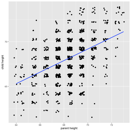<!-- --> --- ## Review of Dispersion Variation (sum of squares) `$$SS = {\sum{(x-\bar{x})^2}}$$` `$$SS = {\sum{(x-\mu)^2}}$$` --- ## Review of Dispersion Variance `$$\large s^{2} = {\frac{\sum{(x-\bar{x})^2}}{N-1}}$$` `$$\large\sigma^{2} = {\frac{\sum{(x-\mu)^2}}{N}}$$` --- ## Review of Dispersion Standard Deviation `$$\large s = \sqrt{\frac{\sum{(x-\bar{x})^2}}{N-1}}$$` `$$\large\sigma = \sqrt{\frac{\sum{(x-\mu)^2}}{N}}$$` --- class: center Formula for standard error of the mean? -- `$$\sigma_M = \frac{\sigma}{\sqrt{N}}$$` `$$\sigma_M = \frac{\hat{s}}{\sqrt{N}}$$` --- ## Associations - i.e., relationships - to look at continuous variable associations we need to think in terms of how variables relate to one another --- ## Associations Covariation (cross products) **Sample:** `$$\large SS = {\sum{(x-\bar{x})(y-\bar{y})}}$$` **Population:** `$$SS = {\sum{{(x-\mu_{x}})(y-\mu_{y})}}$$` --- ## Associations Covariance **Sample:** `$$\large cov_{xy} = {\frac{\sum{(x-\bar{x})(y-\bar{y})}}{N-1}}$$` **Population:** `$$\large \sigma_{xy}^{2} = {\frac{\sum{(x-\mu_{x})(y-\mu_{y})}}{N}}$$` -- >- Covariance matrix is basis for many analyses >- What are some issues that may arise when comparing covariances? --- ## Associations Correlations **Sample:** `$$\large r_{xy} = {\frac{\sum({z_{x}z_{y})}}{N}}$$` **Population:** `$$\large \rho_{xy} = {\frac{cov(X,Y)}{\sigma_{x}\sigma_{y}}}$$` Many other formulas exist for specific types of data, these were more helpful when we computed everything by hand (more on this later). --- ## Correlations - How much two variables are linearly related - -1 to 1 - Invariant to changes in mean or scaling - Most common (and basic) effect size measure - Will use to build our regression model --- ## Correlations 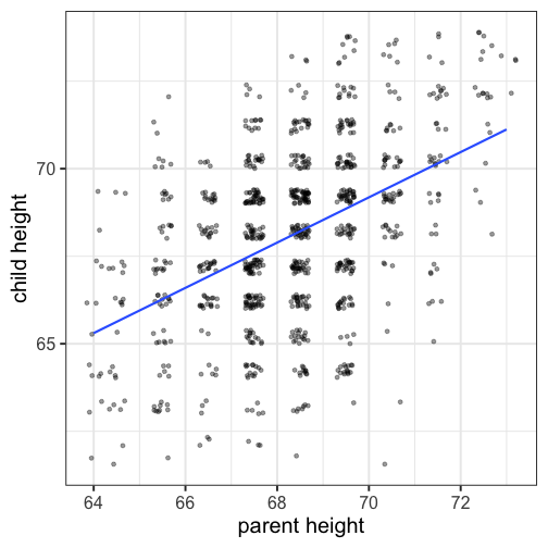<!-- --> --- ## Conceptually Ways to think about a correlation: * How two vectors of numbers co-relate * Product of z-scores + Mathematically, it is * The average squared distance between two vectors in the same space * The cosine of the angle between Y and the projected Y from X `\((\hat{Y})\)`. --- ## Statistical test Hypothesis testing `$$\large H_{0}: \rho_{xy} = 0$$` `$$\large H_{A}: \rho_{xy} \neq 0$$` Assumes: - Observations are independent - Symmetric bivariate distribution (joint probability distribution) --- Univariate distributions 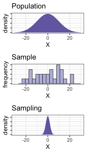<!-- --> --- ### Population <!-- --> --- ### Sample <!-- --> --- ### Sampling distribution? -- The sampling distribution we use depends on our null hypothesis. -- If our null hypothesis is the nil `\((\rho = 0)\)` , then we can use a ***t*-distribution** to estimate the statistical significance of a correlation. --- ## Statistical test Test statistic `$$\large t = {\frac{r}{SE_{r}}}$$` -- .pull-left[ `$$\large SE_r = \sqrt{\frac{1-r^2}{N-2}}$$` `$$\large t = {\frac{r}{\sqrt{\frac{1-r^{2}}{N-2}}}}$$` ] -- .pull-right[ `$$\large DF = N-2$$` ] --- ## Example You're comparing scores on the GRE Quantitative section and GRE Verbal section. You randomly select 30 applications out of those submitted to the University of Oregon and find a correlation between these scores of .80. Is this significantly different from 0? -- `$$\large SE_r = \sqrt{\frac{1-.80^2}{30-2}} = 0.11$$` `$$\large t = \frac{.80}{0.11} = 7.06$$` ```r pt(7.055, df = 30-2, lower.tail = F)*2 ``` ``` ## [1] 0.0000001127696 ``` --- ## Power calculations ```r library(pwr) pwr.r.test(n = , r = .1, sig.level = .05 , power = .8) ``` ``` ## ## approximate correlation power calculation (arctangh transformation) ## ## n = 781.7516 ## r = 0.1 ## sig.level = 0.05 ## power = 0.8 ## alternative = two.sided ``` ```r pwr.r.test(n = , r = .3, sig.level = .05 , power = .8) ``` ``` ## ## approximate correlation power calculation (arctangh transformation) ## ## n = 84.07364 ## r = 0.3 ## sig.level = 0.05 ## power = 0.8 ## alternative = two.sided ``` --- ## Confidence intervals But here's where we get into some trouble. What happens if we try to estimate the precision around our estimate using the techniques we learned in PSY 611? -- For the CI around a mean or a difference in means, we would use: `$$CI_{95} = \bar{X} \pm SE(t_{\text{critical value}})$$` ```r (cv = qt(.975, df = 30-2)) ``` ``` ## [1] 2.048407 ``` ```r .80 - 0.11*cv; .80 + 0.11*cv ``` ``` ## [1] 0.5746752 ``` ``` ## [1] 1.025325 ``` --- ## Fisher's r to z' transformation If we want to make calculations around correlation values that are not equal to 0, then we will run into a skewed sampling distribution. This applies to both calculating confidence intervals around estimates of correlations and null hypotheses in which `\(\rho \neq 0\)`. --- ## Fisher's r to z' transformation <!-- --> --- ## Fisher's r to z' transformation - Skewed sampling distribution will rear its head when: * `\(H_{0}: \rho \neq 0\)` * Calculating confidence intervals * Testing two correlations against one another --- <!-- --> --- ## Fisher’s r to z’ transformation - r to z': `$$\large z^{'} = {\frac{1}{2}}ln{\frac{1+r}{1-r}}$$` --- ## Fisher’s r to z’ transformation <!-- --> --- ## Steps for computing confidence interval 1. Transform r into z' 2. Compute CI as you normally would using z' 3. revert back to r $$ SE_z = \frac{1}{\sqrt{N-3}}$$ `$$\large r = {\frac{e^{2z'}-1}{e^{2z'}+1}}$$` --- ### Example In a sample of 42 students, you calculate a correlation of 0.44 between hours spent outside on Saturday and self-rated health. What is the precision of your estimate? .pull-left[ `$$z = {\frac{1}{2}}ln{\frac{1+.44}{1-.44}} = 0.47$$` `$$SE_z = \frac{1}{\sqrt{42-3}} = 0.16$$` `$$CI_{Z_{LB}} = 0.47-(2.021)0.16 = 0.15$$` `$$CI_{Z_{UB}} = 0.47+(2.021)0.16 = 0.8$$` ] --- .pull-left[ `$$CI_{r_{LB}} = {\frac{e^{2(0.15)}-1}{e^{2(0.15)}+1}} = 0.15$$` `$$CI_{r_{UB}} = = {\frac{e^{2(0.8)}-1}{e^{2(0.8)}+1}} = 0.66$$` These formulas are easy to mistype in R -- use the `psych` package and its functions `fisherz()` and `fisherz2r()` to save time and reduce human error. ] .pull-right[ ```r library(psych) *z_r = fisherz(.44) ``` ``` ## [1] 0.4722308 ``` ```r se = 1/( sqrt(42-3) ) ``` ``` ## [1] 0.1601282 ``` ```r ct = qt(p = .975, df = N-2, lower.tail = T) lbz = z_r - ( se*ct ) ``` ``` ## [1] 0.1485997 ``` ```r *lb = fisherz2r(lbz) ``` ``` ## [1] 0.1475155 ``` ] --- ## Comparing two correlations Again, we use the Fisher’s r to z’ transformation. Here, we're transforming the correlations into z's, then using the difference between z's to calculate the test statistic. `$$Z = \frac{z_1^{'}- z_2^{'}}{se_{z_1-z_2}}$$` `$$se_{z_1-z_2} = \sqrt{se_{z_1}+se_{z_2}} = \sqrt{\frac{1}{n_1-3}+\frac{1}{n_2-3}}$$` --- ## Example You measure narcissism and happiness in two sets of adults: young adults (19-25) and older adults (over 25). You calculate the correlations separately for these two groups, and you want to know whether this relationship is stronger for one group or another. .pull-left[ ### Young adults `$$N = 327$$` `$$r = .402$$` ] .pull-right[ ### Older adults `$$N = 273$$` `$$r = .283$$` ] `$$H_0:\rho_1 = \rho_2$$` `$$H_1:\rho_1 \neq \rho_2$$` --- ```r z1 = fisherz(.402) ``` ``` ## [1] 0.4260322 ``` ```r z2 = fisherz(.283) ``` ``` ## [1] 0.2909403 ``` ```r n1 = 327 n2 = 273 se = sqrt(1/(n1-3) + 1/(n2-3)) ``` ``` ## [1] 0.08240221 ``` ```r zstat = (z1-z2)/se ``` ``` ## [1] 1.639421 ``` ```r pnorm(abs(zstat), lower.tail = F)*2 ``` ``` ## [1] 0.1011256 ``` --- ## Effect size - The strength of relationship between two variables - `\(\eta^2\)`, Cohen’s d, Cohen’s f, hedges g, `\(R^2\)` , Risk-ratio, etc - Significance is a function of effect size and sample size - Statistical significance `\(\neq\)` practical significance --- ## Questions to ask yourself: - What is your N? - What is the typical effect size in the field? - Study design? - What is your DV? - Importance? - Same method as IV (method variance)? --- class: inverse ## Next time... More correlations