class: center, middle, inverse, title-slide # Univariate regression --- ## Last time - Correlation as inferential test - Power - Fisher's r to z transformation - Correlation matrices - Interpreting effect size --- ## Today **Regression** - What is it? Why is it useful - Nuts and bolts - Equation - Ordinary least squares - Interpretation --- ## Regression Regression is a general data analytic system, meaning lots of things fall under the umbrella of regression. This system can handle a variety of forms of relations, although all forms have to be specified in a linear way. Usefully, we can incorporate IVs of all nature -- continuous, categorical, nominal, ordinal.... The output of regression includes both effect sizes and, if using frequentist or Bayesian software, statistical significance. We can also incorporate multiple influences (IVs) and account for their intercorrelations. --- ### Regression - **Adjustment**: Statistically control for known effects + If everyone had the same level of SES, would education still predict wealth? - **Prediction**: We can develop models based on what's happened in the past to predict what will happen in the figure. + Insurance premiums + Graduate school... success? - **Explanation**: explaining the influence of one or more variables on some outcome. + Does this intervention affect reaction time? + Does self-esteem predict relationship quality? --- ## Regression equation What is a regression equation? - Functional relationship - Ideally like a physical law `\((E = MC^2)\)` - In practice, it's never as robust as that. - Note: this equation may not represent the true causal process! How do we uncover the relationship? --- ### How does Y vary with X? - The regression of Y (DV) on X (IV) corresponds to the line that gives the mean value of Y corresponding to each possible value of X - `\(\large E(Y|X)\)` - "Our best guess" regardless of whether our model includes categories or continuous predictor variables --- ## Regression Equation There are two ways to think about our regression equation. They're similar to each other, but they produce different outputs. `$$\Large Y_i = b_{0} + b_{1}X_i +e_i$$` `$$\Large \hat{Y_i} = b_{0} + b_{1}X_i$$` The first is the equation that represents how each **observed outcome** `\((Y_i)\)` is calculated. This observed value is the sum of some constant `\((b_0)\)`, the weighted `\((b_1)\)` observed values of the predictors `\((X_i)\)` and error `\((e_i)\)` that cannot be covered by the observed data. ??? `\(\hat{Y}\)` signifies the fitted score -- no error The difference between the fitted and observed score is the residual ($e_i$) There is a different e value for each observation in the dataset --- ## Regression Equation There are two ways to think about our regression equation. They're similar to each other, but they produce different outputs. `$$\Large Y_i = b_{0} + b_{1}X_i + e_i$$` `$$\Large \hat{Y_i} = b_{0} + b_{1}X_i$$` The second is the equation that represents our expected or **fitted value** of the outcome `\((\hat{Y_i})\)`, sometimes referred to as the "predicted value." This expected value is the sum of some constant `\((b_0)\)`, the weighted `\((b_1)\)` observed values of the predictors `\((X_i)\)`. Note that `\(Y_i - \hat{Y_i} = e\)`. ??? `\(\hat{Y}\)` signifies the fitted score -- no error The difference between the fitted and observed score is the residual ($e_i$) There is a different e value for each observation in the dataset --- ## OLS - How do we find the regression estimates? - Ordinary Least Squares (OLS) estimation - Minimizes deviations $$ min\sum(Y_{i}-\hat{Y})^{2} $$ - Other estimation procedures possible (and necessary in some cases) --- <!-- --> --- <!-- --> --- <!-- --> --- <!-- --> --- ## compare to bad fit .pull-left[ <!-- --> ] .pull-right[ <!-- --> ] --- `$$\Large Y_i = b_{0} + b_{1}X_i +e_i$$` `$$\Large \hat{Y_i} = b_{0} + b_{1}X_i$$` `$$\Large Y_i = \hat{Y_i} + e_i$$` `$$\Large e_i = Y_i - \hat{Y_i}$$` --- ## OLS The line that yields the smallest sum of squared deviations `$$\Large \Sigma(Y_i - \hat{Y_i})^2$$` `$$\Large = \Sigma(Y_i - (b_0+b_{1}X_i))^2$$` `$$\Large = \Sigma(e_i)^2$$` -- In order to find the OLS solution, you could try many different coefficients `\((b_0 \text{ and } b_{1})\)` until you find the one with the smallest sum squared deviation. Luckily, there are simple calculations that will yield the OLS solution every time. --- ## Regression coefficient, `\(b_{1}\)` `$$\large b_{1} = \frac{cov_{XY}}{s_{x}^{2}} = r_{xy} \frac{s_{y}}{s_{x}}$$` <!-- `$$\large r_{xy} = \frac{s_{xy}}{s_xs_y}$$` --> What units is the regression coefficient in? -- The regression coefficient (slope) equals the estimated change in Y for a 1-unit change in X --- `$$\large b_{1} = r_{xy} \frac{s_{y}}{s_{x}}$$` If the variance of both X and Y is equal to 1: `$$\large b_1 = \frac{s_{xy}}{s_xs_y} = \frac{s_{xy}}{s_x^2}=\frac{r_{xy}}{1^2} = \beta_{yx} = b_{yx}^*$$` --- ## Standardized regression equation `$$\large Z_{y_i} = b_{yx}^*Z_{x_i}+e_i$$` `$$\large b_{yx}^* = b_{yx}\frac{s_x}{s_y} = r_{xy}$$` -- According to this regression equation, when `\(X = 0, Y = 0\)`. Our interpretation of the coefficient is that a one-standard deviation increase in X is associated with a `\(b_{yx}^*\)` standard deviation increase in Y. Our regression coefficient is equivalent to the correlation coefficient *when we have only one predictor in our model.* --- ## Estimating the intercept, `\(b_0\)` - intercept serves to adjust for differences in means between X and Y `$$\Large \hat{Y_i} = \bar{Y} + r_{xy} \frac{s_{y}}{s_{x}}(X_i-\bar{X})$$` - if standardized, intercept drops out - otherwise, intercept is where regression line crosses the y-axis at X = 0 ??? ##Make this point - Also, notice that when `\(X = \bar{X}\)` the regression line goes through `\(\bar{Y}\)` ??? `$$\Large b_0 = \bar{Y} - b_1\bar{X}$$` --- The intercept adjusts the location of the regression line to ensure that it runs through the point `\((\bar{X}, \bar{Y}).\)` We can calculate this value using the equation: `$$\Large b_0 = \bar{Y} - b_1\bar{X}$$` --- ## Example [Data on lung cancer rates](https://data.world/nrippner/ols-regression-challenge#) in counties aggregated from American Community Survey, clinicaltrials.gov and cancer.gov. ```r cancer_data = read_csv(here("data/cancer_reg.csv")) describe(cancer_data[,c("avgAnnCount", "medIncome")], fast = T) ``` ``` ## vars n mean sd min max range se ## avgAnnCount 1 3047 606.34 1416.36 6 38150 38144 25.66 ## medIncome 2 3047 47063.28 12040.09 22640 125635 102995 218.12 ``` ```r cor(cancer_data$medIncome, cancer_data$avgAnnCount) ``` ``` ## [1] 0.2691447 ``` --- If we regress cancer rates onto income: ```r r = cor(cancer_data$medIncome, cancer_data$avgAnnCount) m_income = mean(cancer_data$medIncome) m_cancer = mean(cancer_data$avgAnnCount) s_income = sd(cancer_data$medIncome) s_cancer = sd(cancer_data$avgAnnCount) b1 = r*(s_cancer/s_income) ``` ``` ## [1] 0.03166128 ``` ```r b0 = m_cancer - b1*m_income ``` ``` ## [1] -883.7454 ``` How will this change if we regress income onto cancer rates? --- ```r (b1 = r*(s_cancer/s_income)) ``` ``` ## [1] 0.03166128 ``` ```r (b0 = m_cancer - b1*m_income) ``` ``` ## [1] -883.7454 ``` ```r (b1 = r*(s_income/s_cancer)) ``` ``` ## [1] 2.287932 ``` ```r (b0 = m_income - b1*m_cancer) ``` ``` ## [1] 45676.02 ``` --- ## In `R` ```r fit.1 <- lm(avgAnnCount ~ medIncome, data = cancer_data) summary(fit.1) ``` ``` ## ## Call: ## lm(formula = avgAnnCount ~ medIncome, data = cancer_data) ## ## Residuals: ## Min 1Q Median 3Q Max ## -3039 -479 -228 26 37271 ## ## Coefficients: ## Estimate Std. Error t value Pr(>|t|) ## (Intercept) -883.745396 99.738832 -8.861 <0.0000000000000002 *** ## medIncome 0.031661 0.002053 15.421 <0.0000000000000002 *** ## --- ## Signif. codes: 0 '***' 0.001 '**' 0.01 '*' 0.05 '.' 0.1 ' ' 1 ## ## Residual standard error: 1364 on 3045 degrees of freedom ## Multiple R-squared: 0.07244, Adjusted R-squared: 0.07213 ## F-statistic: 237.8 on 1 and 3045 DF, p-value: < 0.00000000000000022 ``` ??? **Things to discuss** - Coefficient estimates - Statistical tests (covered in more detail soon) --- <!-- --> --- ### Data, fitted, and residuals ```r library(broom) model_info = augment(fit.1) head(model_info) ``` ``` ## # A tibble: 6 x 8 ## avgAnnCount medIncome .fitted .resid .std.resid .hat .sigma .cooksd ## <dbl> <dbl> <dbl> <dbl> <dbl> <dbl> <dbl> <dbl> ## 1 1397 61898 1076. 321. 0.235 0.000827 1365. 0.0000229 ## 2 173 48127 640. -467. -0.342 0.000331 1365. 0.0000194 ## 3 102 49348 679. -577. -0.423 0.000340 1365. 0.0000304 ## 4 427 44243 517. -90.0 -0.0660 0.000346 1365. 0.000000755 ## 5 57 49955 698. -641. -0.470 0.000347 1364. 0.0000383 ## 6 428 52313 773. -345. -0.253 0.000391 1365. 0.0000125 ``` ```r describe(model_info, fast = T) ``` ``` ## vars n mean sd min max range se ## avgAnnCount 1 3047 606.34 1416.36 6.00 38150.00 38144.00 25.66 ## medIncome 2 3047 47063.28 12040.09 22640.00 125635.00 102995.00 218.12 ## .fitted 3 3047 606.34 381.20 -166.93 3094.02 3260.95 6.91 ## .resid 4 3047 0.00 1364.09 -3039.02 37270.66 40309.68 24.71 ## .std.resid 5 3047 0.00 1.00 -2.24 27.32 29.57 0.02 ## .hat 6 3047 0.00 0.00 0.00 0.01 0.01 0.00 ## .sigma 7 3047 1364.31 3.63 1185.50 1364.54 179.04 0.07 ## .cooksd 8 3047 0.00 0.00 0.00 0.19 0.19 0.00 ``` ??? Point out the average of the residuals is 0, just like average deviation from the mean is 0. --- ### The relationship between `\(X_i\)` and `\(\hat{Y_i}\)` ```r model_info %>% ggplot(aes(x = medIncome, y = .fitted)) + geom_point() + geom_smooth(se = F, method = "lm") + scale_x_continuous("X") + scale_y_continuous(expression(hat(Y))) + theme_bw(base_size = 30) ``` <!-- --> --- ### The relationship between `\(X_i\)` and `\(e_i\)` ```r model_info %>% ggplot(aes(x = medIncome, y = .resid)) + geom_point() + geom_smooth(se = F, method = "lm") + scale_x_continuous("X") + scale_y_continuous("e") + theme_bw(base_size = 30) ``` <!-- --> --- ### The relationship between `\(Y_i\)` and `\(\hat{Y_i}\)` ```r model_info %>% ggplot(aes(x = avgAnnCount, y = .fitted)) + geom_point() + geom_smooth(se = F, method = "lm") + scale_x_continuous("Y") + scale_y_continuous(expression(hat(Y))) + theme_bw(base_size = 30) ``` 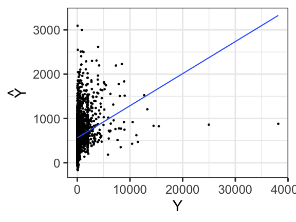<!-- --> --- ### The relationship between `\(Y_i\)` and `\(e_i\)` ```r model_info %>% ggplot(aes(x = avgAnnCount, y = .resid)) + geom_point() + geom_smooth(se = F, method = "lm") + scale_x_continuous("Y") + scale_y_continuous("e") + theme_bw(base_size = 25) ``` 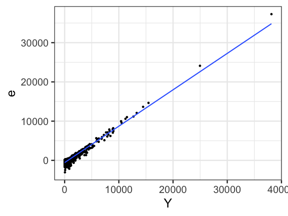<!-- --> --- ### The relationship between `\(\hat{Y_i}\)` and `\(e_i\)` ```r model_info %>% ggplot(aes(x = .fitted, y = .resid)) + geom_point() + geom_smooth(se = F, method = "lm") + scale_y_continuous("e") + scale_x_continuous(expression(hat(Y))) + theme_bw(base_size = 30) ``` 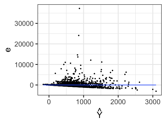<!-- --> --- ## Regression to the mean An observation about heights was part of the motivation to develop the regression equation: If you selected a parent who was exceptionally tall (or short), their child was almost always not as tall (or as short). 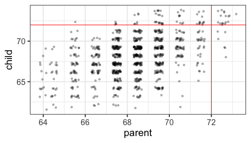<!-- --> --- ## Regression to the mean This phenomenon is known as **regression to the mean.** This describes the phenomenon in which an random variable produces an extreme score on a first measurement, but a lower score on a second measurement. .pull-left[ We can see this in the standardized regression equation: `$$\hat{Y_i} = r_{xy}(X_i) + e_i$$` In that the slope coefficient can never be greater than 1. ] .pull-right[  ] --- ## Regression to the mean This can be a threat to internal validity if interventions are applied based on first measurement scores. .pull-left[ <!-- --> ] -- .pull-right[ <!-- --> ] --- class: inverse ## Next time... Statistical inferences with regression