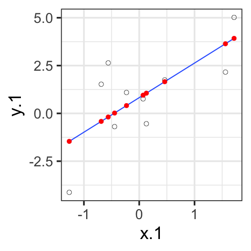
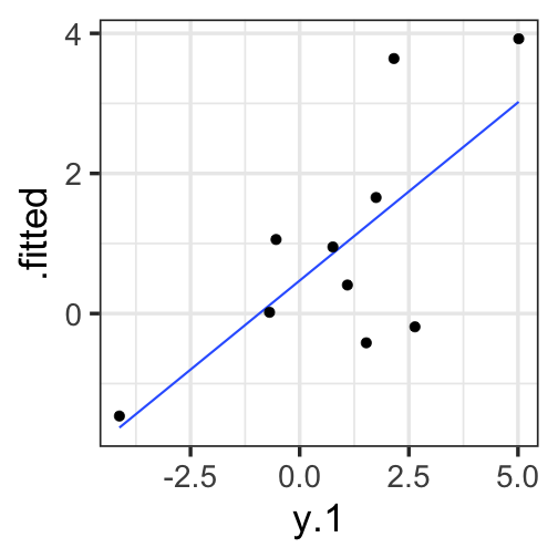
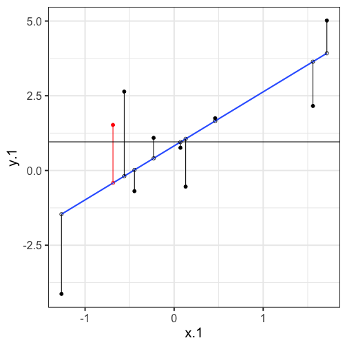
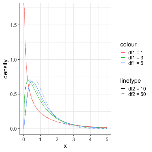
class: center, middle, inverse, title-slide # Univariate regression II --- ## Last time... - Introduction to univariate regression - Calculation and interpretation of `\(b_0\)` and `\(b_1\)` - Relationship between `\(X\)`, `\(Y\)`, `\(\hat{Y}\)`, and `\(e\)` --- ### Today... Statistical inferences with regression - Partitioning variance - Testing `\(b_{xy}\)` --- ## Statistical Inference - The way the world is = our model + error - How good is our model? Does it "fit" the data well? -- To assess how well our model fits the data, we will examine the proportion of variance in our outcome variable that can be "explained" by our model. To do so, we need to partition the variance into different categories. For now, we will partition it into two categories: the variability that is captured by (explained by) our model, and variability that is not. --- ## Partitioning variation We can expand the formula defining the relationship between observed `\(Y\)` and fitted `\(\hat{Y}\)` to represent variability, or sums of squares. `$$Y = \hat{Y} + e$$` `$$Y = \hat{Y} + (Y - \hat{Y})$$` `$$Y - \bar{Y} = (\hat{Y} -\bar{Y}) + (Y - \hat{Y})$$` `$$(Y - \bar{Y})^2 = [(\hat{Y} -\bar{Y}) + (Y - \hat{Y})]^2$$` `$$\sum (Y - \bar{Y})^2 = \sum (\hat{Y} -\bar{Y})^2 + \sum(Y - \hat{Y})^2$$` --- `$$\Large \sum (Y - \bar{Y})^2 = \sum (\hat{Y} -\bar{Y})^2 + \sum(Y - \hat{Y})^2$$` Each of these is the sum of a squared deviation from an expected value of Y. We can abbreviate the sum of squared deviations: `$$\Large SS_Y = SS_{\text{Model}} + SS_{\text{Residual}}$$` The relative magnitude of sums of squares, especially in more complex designs, provides a way of identifying particularly large and important sources of variability. In the future, we can further partition `\(SS_{\text{Model}}\)` and `\(SS_{\text{Residual}}\)` into smaller pieces, which will help us make more specific inferences and increase statistical power, respectively. `$$\Large s^2_Y = s^2_{\hat{Y}} + s^2_{e}$$` --- ## Partitioning variance in Y Consider the case with no correlation between X and Y `$$\Large \hat{Y} = \bar{Y} + r_{xy} \frac{s_{y}}{s_{x}}(X-\bar{X})$$` -- `$$\Large \hat{Y} = \bar{Y}$$` To the extent that we can generate different predicted values of Y based on the values of the predictors, we are doing well in our prediction `$$\large \sum (Y - \bar{Y})^2 = \sum (\hat{Y} -\bar{Y})^2 + \sum(Y - \hat{Y})^2$$` `$$\Large SS_Y = SS_{\text{Model}} + SS_{\text{Residual}}$$` --- ## Coefficient of Determination `$$\Large \frac{s_{Model}^2}{s_{y}^2} = \frac{SS_{Model}}{SS_{Y}} = R^2$$` `\(R^2\)` represents the proportion of variance in Y that is explained by the model. -- `\(\sqrt{R^2} = R\)` is the correlation between the predicted values of Y from the model and the actual values of Y `$$\large \sqrt{R^2} = r_{Y\hat{Y}}$$` --- .pull-left[ <!-- --> ] -- .pull-right[ <!-- --> ] --- ## Example ```r fit.1 = lm(child ~ parent, data = galton.data) summary(fit.1) ``` ``` ## ## Call: ## lm(formula = child ~ parent, data = galton.data) ## ## Residuals: ## Min 1Q Median 3Q Max ## -7.8050 -1.3661 0.0487 1.6339 5.9264 ## ## Coefficients: ## Estimate Std. Error t value Pr(>|t|) ## (Intercept) 23.94153 2.81088 8.517 <0.0000000000000002 *** ## parent 0.64629 0.04114 15.711 <0.0000000000000002 *** ## --- ## Signif. codes: 0 '***' 0.001 '**' 0.01 '*' 0.05 '.' 0.1 ' ' 1 ## ## Residual standard error: 2.239 on 926 degrees of freedom *## Multiple R-squared: 0.2105, Adjusted R-squared: 0.2096 ## F-statistic: 246.8 on 1 and 926 DF, p-value: < 0.00000000000000022 ``` ```r summary(fit.1)$r.squared ``` ``` ## [1] 0.2104629 NA NA NA NA NA NA NA NA NA NA NA NA NA NA *NA``` --- ## Example ```r cor(galton.data$parent, galton.data$child, use = "pairwise") ``` ``` ## [1] 0.4587624 ``` -- ```r cor(galton.data$parent, galton.data$child)^2 ``` ``` ## [1] 0.2104629 ``` --- ## Computing Sum of Squares `$$\Large \frac{SS_{Model}}{SS_{Y}} = R^2$$` `$$\Large SS_{Model} = R^2({SS_{Y})}$$` `$$\Large SS_{residual} = SS_{Y} - R^2({SS_{Y})}$$` `$$\Large SS_{residual} = (1- R^2){SS_{Y}}$$` ??? <!-- --> --- ## residual standard error ``` ## ## Call: ## lm(formula = child ~ parent, data = galton.data) ## ## Residuals: ## Min 1Q Median 3Q Max ## -7.8050 -1.3661 0.0487 1.6339 5.9264 ## ## Coefficients: ## Estimate Std. Error t value Pr(>|t|) ## (Intercept) 23.94153 2.81088 8.517 <0.0000000000000002 *** ## parent 0.64629 0.04114 15.711 <0.0000000000000002 *** ## --- ## Signif. codes: 0 '***' 0.001 '**' 0.01 '*' 0.05 '.' 0.1 ' ' 1 ## *## Residual standard error: 2.239 on 926 degrees of freedom ## Multiple R-squared: 0.2105, Adjusted R-squared: 0.2096 ## F-statistic: 246.8 on 1 and 926 DF, p-value: < 0.00000000000000022 ``` --- ## residual standard error/deviation - aka standard deviation of the residual - aka **standard error of the estimate** `$$\hat{\sigma} = \sqrt{\frac{SS_{\text{Residual}}}{df_{\text{Residual}}}} = s_{Y|X} = \sqrt{\frac{\Sigma(Y_i -\hat{Y_i})^2}{N-2}}$$` - interpreted in original units (unlike `\(R^2\)`) - standard deviation of Y not accounted by model --- ## residual standard error/deviation or standard error of the estimate ```r summary(fit.1)$sigma ``` ``` ## [1] 2.238547 ``` ```r galton.data.1 = broom::augment(fit.1) psych::describe(galton.data.1$.resid) ``` ``` ## vars n mean sd median trimmed mad min max range skew kurtosis se ## X1 1 928 0 2.24 0.05 0.06 2.26 -7.81 5.93 13.73 -0.24 -0.23 0.07 ``` ```r sd(galton.data$child) ``` ``` ## [1] 2.517941 ``` --- ## `\(R^2\)` and residual standard deviation - two sides of same coin - one in original units (residual standard deviation), the other standardized `\((R^2)\)` --- ## Inferential tests NHST is about making decisions: - these two means are/are not different - this correlation is/is not significant - the distribution of this categorical variable is/is not different between these groups -- In regression, there are several inferential tests being conducted at once. The first is called the **omnibus test** -- this is a test of whether the model fits the data. --- ### Omnibus test <!-- `$$\Large H_{0}: \rho_{Y\hat{Y}}^2= 0$$` --> <!-- `$$\Large H_{0}: \rho_{Y\hat{Y}}^2 \neq 0$$` --> Historically we use **the _F_ distribution** to estimate the significance of our model, because it works with our ability to partition variance. What is our null hypothesis? **The model does not account for variance in `\(Y\)`.** -- But you can also think of the null hypothesis as `$$\Large H_{0}: \rho_{Y\hat{Y}}^2= 0$$` --- <!-- --> --- ## _F _ Distribution review The F probability distribution represents all possible ratios of two variances: `$$F \approx \frac{s^2_{1}}{s^2_{2}}$$` Each variance estimate in the ratio is `\(\chi^2\)` distributed, if the data are normally distributed. The ratio of two `\(\chi^2\)` distributed variables is `\(F\)` distributed. It should be noted that each `\(\chi^2\)` distribution has its own degrees of freedom. `$$F_{\nu_1\nu_2} = \frac{\frac{\chi^2_{\nu_1}}{\nu_1}}{\frac{\chi^2_{\nu_2}}{\nu_2}}$$` As a result, _F_ has two degrees of freedom, `\(\nu_1\)` and `\(\nu_2\)` ??? --- ## _F_ Distributions and regression Recall that when using a _z_ or _t_ distribution, we were interested in whether one mean was equal to another mean -- sometimes the second mean was calculated from another sample or hypothesized (i.e., the value of the null). In this comparison, we compared the _difference of two means_ to 0 (or whatever our null hypothesis dictates), and if the difference was not 0, we concluded significance. _F_ statistics are not testing the likelihood of differences; they test the size of a _ratio_. In this case, we want to determine whether the variance explained by our model is larger in magnitude than another variance. Which variance? --- `$$\Large F_{\nu_1\nu_2} = \frac{\frac{\chi^2_{\nu_1}}{\nu_1}}{\frac{\chi^2_{\nu_2}}{\nu_2}}$$` `$$\Large F_{\nu_1\nu_2} = \frac{\frac{\text{Variance}_{\text{Model}}}{\nu_1}}{\frac{\text{Variance}_{\text{Residual}}}{\nu_2}}$$` `$$\Large F = \frac{MS_{Model}}{MS_{residual}}$$` --- .pull-left[ The degrees of freedom for our model are `$$DF_1 = k$$` `$$DF_2 = N-k-1$$` Where k is the number of IV's in your model, and N is the sample size. ] .pull-right[ Mean squares are calculated by taking the relevant Sums of Squares and dividing by their respective degrees of freedom. - `\(SS_{\text{Model}}\)` is divided by `\(DF_1\)` - `\(SS_{\text{Residual}}\)` is divided by `\(DF_2\)` ] --- ```r anova(fit.1) ``` ``` ## Analysis of Variance Table ## ## Response: child ## Df Sum Sq Mean Sq F value Pr(>F) ## parent 1 1236.9 1236.93 246.84 < 0.00000000000000022 *** ## Residuals 926 4640.3 5.01 ## --- ## Signif. codes: 0 '***' 0.001 '**' 0.01 '*' 0.05 '.' 0.1 ' ' 1 ``` --- ```r summary(fit.1) ``` ``` ## ## Call: ## lm(formula = child ~ parent, data = galton.data) ## ## Residuals: ## Min 1Q Median 3Q Max ## -7.8050 -1.3661 0.0487 1.6339 5.9264 ## ## Coefficients: ## Estimate Std. Error t value Pr(>|t|) ## (Intercept) 23.94153 2.81088 8.517 <0.0000000000000002 *** ## parent 0.64629 0.04114 15.711 <0.0000000000000002 *** ## --- ## Signif. codes: 0 '***' 0.001 '**' 0.01 '*' 0.05 '.' 0.1 ' ' 1 ## ## Residual standard error: 2.239 on 926 degrees of freedom ## Multiple R-squared: 0.2105, Adjusted R-squared: 0.2096 *## F-statistic: 246.8 on 1 and 926 DF, p-value: < 0.00000000000000022 ``` --- ## Mean square error (MSE) - AKA means square residual/within - unbiased estimate of error variance - measure of discrepancy between the data and the model - the MSE is the variance around the fitted regression line - Note: this is not the same thing as the residual standard error --- ## regression coefficient `$$\Large H_{0}: \beta_{1}= 0$$` `$$\Large H_{1}: \beta_{1} \neq 0$$` --- ## What does the regression coefficient test? - Does X provide any predictive information? - Does X provide any explanatory power regarding the variability of Y? - Is the the average value the best guess (i.e., is Y bar equal to the predicted value of Y?) - Is the regression line flat? - Are X and Y correlated? --- ## Regression coefficient `$$\Large se_{b} = \frac{s_{Y}}{s_{X}}{\sqrt{\frac {1-r_{xy}^2}{n-2}}}$$` `$$\Large t(n-2) = \frac{b_{1}}{se_{b}}$$` --- ## `\(SE_b\)` - standard errors for the slope coefficient - represent our uncertainty (noise) in our estimate of the regression coefficient - different from residual standard error/deviation (but proportional to) - much like previously we can take our estimate (b) and put confidence regions around it to get an estimate of what could be "possible" if we ran the study again --- ## Intercept - more complex standard error calculation as the calculation depends on how far the X value (here zero) is away from the mean of X - farther from the mean, less information, thus more uncertainty --- ```r summary(fit.1) ``` ``` ## ## Call: ## lm(formula = child ~ parent, data = galton.data) ## ## Residuals: ## Min 1Q Median 3Q Max ## -7.8050 -1.3661 0.0487 1.6339 5.9264 ## ## Coefficients: ## Estimate Std. Error t value Pr(>|t|) *## (Intercept) 23.94153 2.81088 8.517 <0.0000000000000002 *** *## parent 0.64629 0.04114 15.711 <0.0000000000000002 *** ## --- ## Signif. codes: 0 '***' 0.001 '**' 0.01 '*' 0.05 '.' 0.1 ' ' 1 ## ## Residual standard error: 2.239 on 926 degrees of freedom ## Multiple R-squared: 0.2105, Adjusted R-squared: 0.2096 ## F-statistic: 246.8 on 1 and 926 DF, p-value: < 0.00000000000000022 ``` --- class: inverse ## Next time... Even more univariate regression! -- - Confidence intervals - Confidence and prediction _bands_ - Model comparison - **Matrix algebra**