Univariate regression III

class: center, middle, inverse, title-slide

# Univariate regression III

---

## Last week

.pull-left[

**Unstandardized regression equation**

`$$Y = b_0 + b_1X + e$$`

- Intercept and slope are interpreted in the units of Y.
  - Useful if the units of Y are meaningful. (Dollars, days, donuts)
  
- Built from covariances and variances

`$$b_1 = \frac{cov_{XY}}{s^2_X}$$`

]

.pull-right[

**Standardized regression equation**

`$$Z_Y = b^*_1Z_X + e$$`

- Slope are interpreted in standardized units.
  - Useful for comparison
  
- Built from correlations

`$$b^*_1 = r_{xy}$$`

]

---

## Last week -- Inferential tests

.pull-left[
**Omnibus test**

- Does the model fit the data?

- *F*-test (ratio of variances)

- How many magnitudes larger is variability attributed to the model compared to left-over variability?
    
* Effect size: Model fit can be measured in terms of `$\large R^2$` or `$\large s_{Y|X}$`
  ]

---
## Terminology

- `$R^2$`
--
  - **coefficient of determination**
  - squared correlation between `$Y$` and `$\hat{Y}$`
  - proportion of variance in Y accounted for by the model
  
- `$s_{Y|X}$`

--
  - **standard error of the estimate** or standard deviation of the residuals.
  - The standard deviation of Y not accounted for by the model. (Compare this to the original standard deviation.)
  
- `$MSE$`

--
  - **mean square error** or unbiased estimate of error variance
  - measure of discrepancy between model and data
  - variance around fitted regression line

---

## Example
 
*Overclaiming* occurs when people claim that they know something that is impossible to know; are experts susceptible to overclaiming?

Participants completed a measure of self-perceived knowledge, in which they indicate their level of knowledge in the area of personal finance. Next participants indicated how much they knew about 15 terms related to personal finance (e.g., home equity). Included in the 15 items were three terms that do not actually exist (e.g., annualized credit). Thus, overclaiming occurred when participants said that they were knowledgeable about the non-existent terms. Finally, participants completed a test of financial literacy called the FINRA.

.small[
Atir, S., Rosenzweig, E., & Dunning, D. (2015). [When knowledge knows no bounds: Self-perceived expertise predicts claims of impossible knowledge.](https://journals.sagepub.com/stoken/default+domain/ZtrwAQcGwtzhkvv8vgKq/full) Psychological Science, 26, 1295-1303. ]

---

```r
library(here)
expertise = read.csv(here("data/expertise.csv"))
psych::describe(expertise)
```

```
##                          vars   n   mean    sd median trimmed   mad   min
## id                          1 202 101.50 58.46 101.50  101.50 74.87  1.00
## order_of_tasks              2 202   1.50  0.50   1.50    1.50  0.74  1.00
*## self_perceived_knowledge    3 202   4.43  1.17   4.50    4.45  0.74  1.00
*## overclaiming_proportion     4 202   0.31  0.23   0.28    0.29  0.25  0.00
## accuracy                    5 202   0.30  0.21   0.28    0.29  0.21 -0.19
## FINRA_score                 6 202   3.70  1.19   4.00    3.85  1.48  0.00
##                             max  range  skew kurtosis   se
## id                       202.00 201.00  0.00    -1.22 4.11
## order_of_tasks             2.00   1.00  0.00    -2.01 0.04
## self_perceived_knowledge   7.00   6.00 -0.20     0.15 0.08
## overclaiming_proportion    1.00   1.00  0.64    -0.31 0.02
## accuracy                   0.93   1.12  0.28    -0.07 0.01
## FINRA_score                5.00   5.00 -1.01     0.57 0.08
```

```r
cor(expertise[,c("self_perceived_knowledge", "overclaiming_proportion")])
```

```
##                          self_perceived_knowledge overclaiming_proportion
## self_perceived_knowledge                1.0000000               0.4811502
## overclaiming_proportion                 0.4811502               1.0000000
```

---

```r
fit.1 = lm(overclaiming_proportion ~ self_perceived_knowledge, 
           data = expertise)
anova(fit.1)
```

```
## Analysis of Variance Table
## 
## Response: overclaiming_proportion
##                           Df Sum Sq Mean Sq F value             Pr(>F)    
## self_perceived_knowledge   1 2.5095 2.50948  60.249 0.0000000000004225 ***
## Residuals                200 8.3303 0.04165                               
## ---
## Signif. codes:  0 '***' 0.001 '**' 0.01 '*' 0.05 '.' 0.1 ' ' 1
```

---

```r
summary(fit.1)
```

```
## 
## Call:
## lm(formula = overclaiming_proportion ~ self_perceived_knowledge, 
##     data = expertise)
## 
## Residuals:
##      Min       1Q   Median       3Q      Max 
## -0.50551 -0.15610  0.00662  0.12167  0.54215 
## 
## Coefficients:
##                          Estimate Std. Error t value          Pr(>|t|)    
## (Intercept)              -0.11406    0.05624  -2.028            0.0439 *  
## self_perceived_knowledge  0.09532    0.01228   7.762 0.000000000000422 ***
## ---
## Signif. codes:  0 '***' 0.001 '**' 0.01 '*' 0.05 '.' 0.1 ' ' 1
## 
## Residual standard error: 0.2041 on 200 degrees of freedom
## Multiple R-squared:  0.2315,	Adjusted R-squared:  0.2277 
## F-statistic: 60.25 on 1 and 200 DF,  p-value: 0.0000000000004225
```

---
.pull-left[

```r
library(sjPlot)
set_theme(base = theme_bw())
plot_model(fit.1, 
           type = "pred", 
           show.data = T)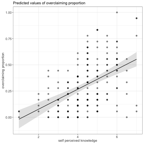 
```

![](5-regression_files/figure-html/unnamed-chunk-6-1.png)
]

.pull-right[

```r
plot_model(fit.1, 
           type = "pred", 
           show.data = T, 
           jitter = T)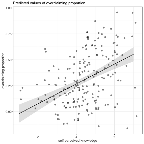 
```

![](5-regression_files/figure-html/unnamed-chunk-7-1.png)
]

---

## regression coefficient

`$$\Large H_{0}: \beta_{1}= 0$$`
`$$\Large H_{1}: \beta_{1} \neq 0$$`

---

## What does the regression coefficient test?

- Does X provide any predictive information?

- Does X provide any explanatory power regarding the variability of Y?

- Is the the average value the best guess (i.e., is Y bar equal to the predicted value of Y?)

- Is the regression line flat?

- Are X and Y correlated?

---

## Regression coefficient
`$$\Large se_{b} = \frac{s_{Y}}{s_{X}}{\sqrt{\frac {1-r_{xy}^2}{n-2}}}$$`
`$$\Large t(n-2) = \frac{b_{1}}{se_{b}}$$`

---

```r
summary(fit.1)
```

```
## 
## Call:
## lm(formula = overclaiming_proportion ~ self_perceived_knowledge, 
##     data = expertise)
## 
## Residuals:
##      Min       1Q   Median       3Q      Max 
## -0.50551 -0.15610  0.00662  0.12167  0.54215 
## 
## Coefficients:
##                          Estimate Std. Error t value          Pr(>|t|)    
## (Intercept)              -0.11406    0.05624  -2.028            0.0439 *  
*## self_perceived_knowledge  0.09532    0.01228   7.762 0.000000000000422 ***
## ---
## Signif. codes:  0 '***' 0.001 '**' 0.01 '*' 0.05 '.' 0.1 ' ' 1
## 
## Residual standard error: 0.2041 on 200 degrees of freedom
## Multiple R-squared:  0.2315,	Adjusted R-squared:  0.2277 
## F-statistic: 60.25 on 1 and 200 DF,  p-value: 0.0000000000004225
```

---

## `$SE_b$`

- standard errors for the slope coefficient

- represent our uncertainty (noise) in our estimate of the regression coefficient

- different from residual standard error/deviation (but proportional to)

- much like previously we can take our estimate (b) and put confidence regions around it to get an estimate of what could be "possible" if we ran the study again

---
## Intercept

- more complex standard error calculation as the calculation depends on how far the X value (here zero) is away from the mean of X

- farther from the mean, less information, thus more uncertainty 
    
---

```r
summary(fit.1)
```

```
## 
## Call:
## lm(formula = overclaiming_proportion ~ self_perceived_knowledge, 
##     data = expertise)
## 
## Residuals:
##      Min       1Q   Median       3Q      Max 
## -0.50551 -0.15610  0.00662  0.12167  0.54215 
## 
## Coefficients:
##                          Estimate Std. Error t value          Pr(>|t|)    
*## (Intercept)              -0.11406    0.05624  -2.028            0.0439 *  
## self_perceived_knowledge  0.09532    0.01228   7.762 0.000000000000422 ***
## ---
## Signif. codes:  0 '***' 0.001 '**' 0.01 '*' 0.05 '.' 0.1 ' ' 1
## 
## Residual standard error: 0.2041 on 200 degrees of freedom
## Multiple R-squared:  0.2315,	Adjusted R-squared:  0.2277 
## F-statistic: 60.25 on 1 and 200 DF,  p-value: 0.0000000000004225
```

---
## Confidence interval for coefficients

- same equation as we've been working with:

`$$CI_b = b \pm CV(SE_b)$$`

- How do we estimate the critical value?

- After a certain sample size, the CV can be assumed to be what?

---
## `$SE_{\hat{Y_i}}$`

In addition to estimating precision around the our coefficients, we can also estimate our precision around our predicted values, `$\hat{Y_i}$`. Why might this be a useful exercise?

The formula to estimate the standard error of any particular `$\hat{Y_i}$` is

`$$s_{\hat{Y}_X} = s_{Y|X}*\sqrt{\frac {1}{n}+\frac{(X-\bar{X})^2}{(n-1)s_{X}^2}}$$`
---

```r
library(broom)
model_info = augment(fit.1, se_fit = T)
psych::describe(model_info, fast=T)
```

```
##                          vars   n mean   sd   min  max range   se
## overclaiming_proportion     1 202 0.31 0.23  0.00 1.00  1.00 0.02
## self_perceived_knowledge    2 202 4.43 1.17  1.00 7.00  6.00 0.08
## .fitted                     3 202 0.31 0.11 -0.02 0.55  0.57 0.01
*## .se.fit                     4 202 0.02 0.01  0.01 0.04  0.03 0.00
## .resid                      5 202 0.00 0.20 -0.51 0.54  1.05 0.01
## .std.resid                  6 202 0.00 1.00 -2.50 2.68  5.18 0.07
## .hat                        7 202 0.01 0.01  0.00 0.05  0.04 0.00
## .sigma                      8 202 0.20 0.00  0.20 0.20  0.00 0.00
## .cooksd                     9 202 0.01 0.01  0.00 0.09  0.09 0.00
```

```r
head(model_info[,c(".fitted", ".se.fit")])
```

```
## # A tibble: 6 x 2
##   .fitted .se.fit
##     <dbl>   <dbl>
## 1   0.410  0.0195
## 2   0.315  0.0144
## 3   0.220  0.0183
## 4   0.458  0.0241
## 5   0.124  0.0277
## 6   0.553  0.0347
```

We can string these together in a figure and create **confidence bands**.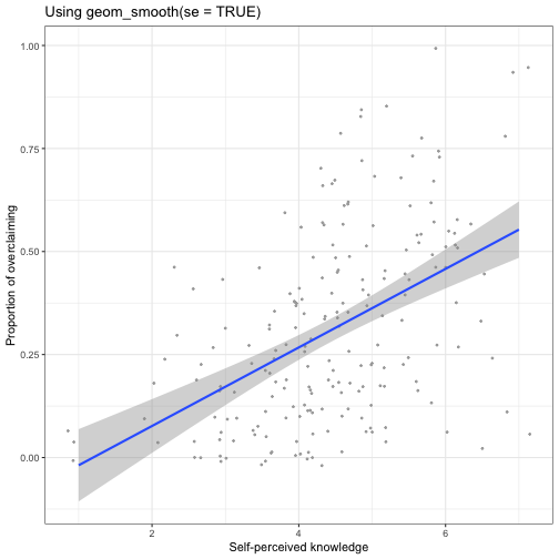

---

![](5-regression_files/figure-html/unnamed-chunk-12-1.png)

---

```r
confint(fit.1)
```

```
##                                2.5 %       97.5 %
## (Intercept)              -0.22495982 -0.003151603
## self_perceived_knowledge  0.07110265  0.119532290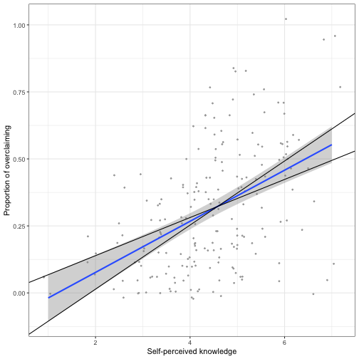
```

---

![](5-regression_files/figure-html/unnamed-chunk-14-1.png)

---
## Confidence Bands for regression line
![](5-regression_files/figure-html/unnamed-chunk-15-1.png)
---
Compare mean estimate for self-perceived knowledge based on regression vs binning

![](5-regression_files/figure-html/unnamed-chunk-16-1.png)
---
## Confidence Bands

`$$\Large \hat{Y}\pm t_{critical} * s_{Y|X}*\sqrt{\frac {1}{n}+\frac{(X-\bar{X})^2}{(n-1)s_{X}^2}}$$`

---
## Prediction bands

`$$\large \hat{Y}\pm t_{critical} * se_{residual}*\sqrt{1+ \frac {1}{n}+\frac{(X-\bar{X})^2}{(n-1)s_{X}^2}}$$`

- predicting and individual `$i's$` score, not the `$\hat{Y}$` for a particular level of X. (A new `$Y_i$` given x, rather than `$\bar{Y}$` given x)

- Because there is greater variation in predicting an individual value rather than a collection of individual values (i.e., the mean) the prediction band is greater

- Combines unknown variability of the estimated mean `$(\text{as reflected in }SE_b)$` with peoples' scores around mean `$(\text{residual standard error }, s_{Y|X})$`

---

![](5-regression_files/figure-html/unnamed-chunk-17-1.png)

---

## Matrix algebra

Matrix algebra serves several uses here. First, it can help us to visualize our regression equation in terms of data:

`$$\small \left[\begin{array}
{r}
y_1   \\
y_2   \\
\dots \\
y_n   
\end{array}\right]
=
\left[\begin{array}
{rrr}
b_{0} & b_{1}
\end{array}\right] 
\times 
\left[\begin{array}
{rr}
1 & x_1   \\
1 & x_2   \\
\dots \\
1 & x_n   
\end{array}\right]
+
\left[\begin{array}
{r}
e_1   \\
e_2   \\
\dots \\
e_n   
\end{array}\right]$$`

---

## Matrix algebra

Recall that `$Y$` is a vector of values, which can be represented as an `$n\times1$` matrix, `$\mathbf{y}$`. Similarly, X can be represented as an `$n\times1$` matrix, `$\mathbf{X}$`.

Consider now our regression equation:

`$$\mathbf{y} = b_0 + b_1\mathbf{x} + e$$`

If we augment the matrix `$\mathbf{X}$` to be an `$n\times2$` matrix, in which the first column is filled with 1's, we can simplify this equation:

`$$\mathbf{y} = \mathbf{b}\mathbf{X}$$`

Where `$\mathbf{b}$` is a `$1 \times 2$` matrix containing our estimates of the intercept and slope. If we solve for b, we find that

`$$(\mathbf{X'X})^{-1} \mathbf{X'y}=\mathbf{b}$$`

???
One property of the residuals is that the the average residual is 0, so we can remove this from the equation as well.

---

### A "simple" example

.pull-left[
| X | 6 | 7 | 8 | 9 | 7 |
|:-:|:-:|:-:|:-:|:-:|:-:|
| Y | 1 | 2 | 3 | 3 | 4 |
]

.pull-right[
`$$\mathbf{X} = \left(\begin{array}
{rr}
1 & 6  \\
1 & 7 \\
1 & 8 \\
1 & 9 \\
1 & 7 \\
\end{array}\right)$$`
]

`$$\mathbf{X'X} = \left(\begin{array}
{rrrrr}
1 & 1 & 1 & 1 & 1  \\
6 & 7 & 8 & 9 & 7 \\
\end{array}\right) \left(\begin{array}
{rr}
1 & 6  \\
1 & 7 \\
1 & 8 \\
1 & 9 \\
1 & 7 \\
\end{array}\right) = 
\left(\begin{array}
{rr}
5 & 37  \\
37 & 279 \\
\end{array}\right)$$`

???

$$
\mathbf{X'X} = \left(\begin{array}
{rr}
N & \Sigma X  \\
\Sigma X & \Sigma X^2 \\
\end{array}\right)
$$

---

`$$\mathbf{X'X} = 
\left(\begin{array}
{rr}
5 & 37  \\
37 & 279 \\
\end{array}\right)$$`

```r
m = matrix(c(5,37,37,279), nrow = 2)
solve(m)
```

```
##           [,1]       [,2]
## [1,] 10.730769 -1.4230769
## [2,] -1.423077  0.1923077
```

`$$(\mathbf{X'X})^{-1} = 
\left(\begin{array}
{rr}
10.73 & -1.42  \\
-1.42 & .19 \\
\end{array}\right)$$`

---

.pull-left[
`$$\mathbf{X} = \left(\begin{array}
{rr}
1 & 6  \\
1 & 7 \\
1 & 8 \\
1 & 9 \\
1 & 7 \\
\end{array}\right)$$`
]
.pull-right[
`$$\mathbf{y} = \left(\begin{array}
{r}
1   \\
2  \\
3  \\
3  \\
4  \\
\end{array}\right)$$`
]

`$$\mathbf{X'y} = \left(\begin{array}
{rrrrr}
1 & 1 & 1 & 1 & 1  \\
6 & 7 & 8 & 9 & 7 \\
\end{array}\right) \left(\begin{array}
{r}
1   \\
2  \\
3  \\
3  \\
4  \\
\end{array}\right) = 
\left(\begin{array}
{r}
13   \\
99 \\
\end{array}\right)$$`

???

$$
\mathbf{X'y} = \left(\begin{array}
{rr}
\Sigma Y   \\
\Sigma XY  \\
\end{array}\right)
$$
---
`$$(\mathbf{X'X})^{-1} \mathbf{X'y}=\mathbf{b}$$`

`$$\mathbf{X'y} = \left(\begin{array}
{rr}
10.73 & -1.42   \\
-1.42 & .19  \\
\end{array}\right) \left(\begin{array}
{r}
13   \\
99  \\
\end{array}\right) = 
\left(\begin{array}
{r}
-1.38   \\
0.54 \\
\end{array}\right)$$`

```r
x = c(6,7,8,9,7)
y = c(1,2,3,3,4)
summary(lm(y ~ x))
```

```
## 
## Call:
## lm(formula = y ~ x)
## 
## Residuals:
##        1        2        3        4        5 
## -0.84615 -0.38462  0.07692 -0.46154  1.61538 
## 
## Coefficients:
##             Estimate Std. Error t value Pr(>|t|)
## (Intercept)  -1.3846     3.6342  -0.381    0.729
## x             0.5385     0.4865   1.107    0.349
## 
## Residual standard error: 1.109 on 3 degrees of freedom
## Multiple R-squared:  0.2899,	Adjusted R-squared:  0.05325 
## F-statistic: 1.225 on 1 and 3 DF,  p-value: 0.3492
```

---

## Matrix algebra

In the case of a single predictor (univariate regression), the matrix algebra method to calculate coefficients may seem more complicated than using the formulas for OLS. (See [here](https://www.stat.purdue.edu/~boli/stat512/lectures/topic3.pdf) for formulas showing how they're the same.)

However, when we expand into multiple regression (next week), the matrix algebra method is much easier to expand to fit.

Matrix algebra can [explain *why* our formulas](https://www.stat.cmu.edu/~cshalizi/mreg/15/lectures/13/lecture-13.pdf) for the intercept and slope generate the regression line with the smallest squared error.

---
## Model Comparison

- The basic idea is asking how much variance remains unexplained in our model. This "left over" variance can be contrasted with an alternative model/hypothesis. We can ask does adding a new predictor variable help explain more variance or should we stick with a parsimonious model.

- Every test of an omnibus model is implicitly a model comparisons, typically of your fitted model with the nil model (no slopes). This framework allows you to be more flexible and explicit.

---

```r
fit.1 <- lm(overclaiming_proportion ~ self_perceived_knowledge, 
            data = expertise)

fit.0 <- lm(overclaiming_proportion ~ 1,
            data = expertise)
```

---

```r
summary(fit.0)
```

```
## 
## Call:
## lm(formula = overclaiming_proportion ~ 1, data = expertise)
## 
## Residuals:
##      Min       1Q   Median       3Q      Max 
## -0.30803 -0.19692 -0.03025  0.13641  0.69197 
## 
## Coefficients:
##             Estimate Std. Error t value            Pr(>|t|)    
## (Intercept)  0.30803    0.01634   18.85 <0.0000000000000002 ***
## ---
## Signif. codes:  0 '***' 0.001 '**' 0.01 '*' 0.05 '.' 0.1 ' ' 1
## 
## Residual standard error: 0.2322 on 201 degrees of freedom
```

---

```r
summary(fit.1)
```

---

```r
anova(fit.0)
```

```
## Analysis of Variance Table
## 
## Response: overclaiming_proportion
##            Df Sum Sq  Mean Sq F value Pr(>F)
## Residuals 201  10.84 0.053929
```

---

```r
anova(fit.1)
```

---

```r
anova(fit.1, fit.0)
```

```
## Analysis of Variance Table
## 
## Model 1: overclaiming_proportion ~ self_perceived_knowledge
## Model 2: overclaiming_proportion ~ 1
##   Res.Df     RSS Df Sum of Sq      F             Pr(>F)    
## 1    200  8.3303                                           
## 2    201 10.8398 -1   -2.5095 60.249 0.0000000000004225 ***
## ---
## Signif. codes:  0 '***' 0.001 '**' 0.01 '*' 0.05 '.' 0.1 ' ' 1
```
---
## Model Comparisons

- Model comparisons are redundant with nil/null hypotheses and coefficient tests right now, but will be more flexible down the road.

- Key is to start thinking about your implicit alternative models

- The ultimate goal would be to create two models that represent two equally plausible theories.

- Theory A is made up of components XYZ, whereas theory B has QRS components. You can then ask which theory (model) is better?

---
class: inverse

## Next time

The general linear model