class: center, middle, inverse, title-slide # Univariate regression --- ## Last time - Correlation as inferential test - Power - Fisher's r to z transformation - Correlation matrices - Interpreting effect size --- ## Today **Regression** - What is it? Why is it useful - Nuts and bolts - Equation - Ordinary least squares - Interpretation --- ## Regression Regression is a general data analytic system, meaning lots of things fall under the umbrella of regression. This system can handle a variety of forms of relations, although all forms have to be specified in a linear way. Usefully, we can incorporate IVs of all nature -- continuous, categorical, nominal, ordinal.... The output of regression includes both effect sizes and, if using frequentist or Bayesian software, statistical significance. We can also incorporate multiple influences (IVs) and account for their intercorrelations. --- ### Regression - **Adjustment**: Statistically control for known effects + If everyone had the same level of SES, would education still predict wealth? - **Prediction**: We can develop models based on what's happened in the past to predict what will happen in the future. + Insurance premiums + Graduate school... success? - **Explanation**: explaining the influence of one or more variables on some outcome. + Does this intervention affect reaction time? + Does self-esteem predict relationship quality? --- ## Regression equation What is a regression equation? - Functional relationship - Ideally like a physical law `\((E = MC^2)\)` - In practice, it's never as robust as that. - Note: this equation may not represent the true causal process! How do we uncover the relationship? --- ### How does Y vary with X? - The regression of Y (DV) on X (IV) corresponds to the line that gives the mean value of Y corresponding to each possible value of X - `\(\large E(Y|X)\)` - "Our best guess" regardless of whether our model includes categories or continuous predictor variables --- ## Regression Equation There are two ways to think about our regression equation. They're similar to each other, but they produce different outputs. `$$\Large Y_i = b_{0} + b_{1}X_i +e_i$$` `$$\Large \hat{Y_i} = b_{0} + b_{1}X_i$$` The first is the equation that represents how each **observed outcome** `\((Y_i)\)` is calculated. This observed value is the sum of some constant `\((b_0)\)`, the weighted `\((b_1)\)` observed values of the predictors `\((X_i)\)` and error `\((e_i)\)` that cannot be covered by the observed data. ??? `\(\hat{Y}\)` signifies the fitted score -- no error The difference between the fitted and observed score is the residual ($e_i$) There is a different e value for each observation in the dataset --- ## Regression Equation There are two ways to think about our regression equation. They're similar to each other, but they produce different outputs. `$$\Large Y_i = b_{0} + b_{1}X_i + e_i$$` `$$\Large \hat{Y_i} = b_{0} + b_{1}X_i$$` The second is the equation that represents our expected or **fitted value** of the outcome `\((\hat{Y_i})\)`, sometimes referred to as the "predicted value." This expected value is the sum of some constant `\((b_0)\)`, the weighted `\((b_1)\)` observed values of the predictors `\((X_i)\)`. Note that `\(Y_i - \hat{Y_i} = e_i\)`. ??? `\(\hat{Y}\)` signifies the fitted score -- no error The difference between the fitted and observed score is the residual ($e_i$) There is a different e value for each observation in the dataset --- ## OLS - How do we find the regression estimates? - Ordinary Least Squares (OLS) estimation - Minimizes deviations $$ min\sum(Y_{i}-\hat{Y})^{2} $$ - Other estimation procedures possible (and necessary in some cases) --- <!-- --> --- <!-- --> --- <!-- --> --- <!-- --> --- ## compare to bad fit .pull-left[ <!-- --> ] .pull-right[ 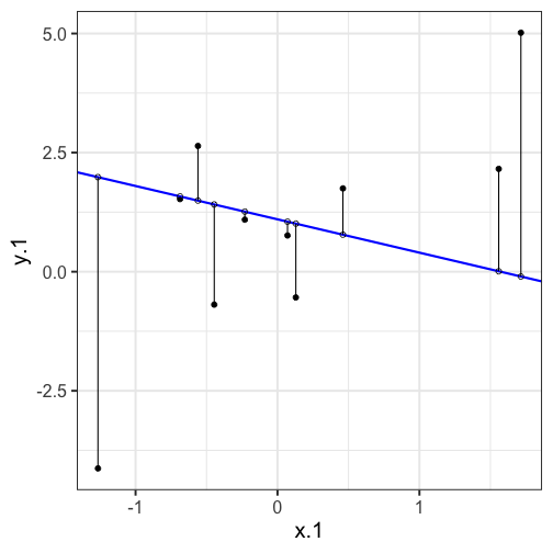<!-- --> ] --- `$$\Large Y_i = b_{0} + b_{1}X_i +e_i$$` `$$\Large \hat{Y_i} = b_{0} + b_{1}X_i$$` `$$\Large Y_i = \hat{Y_i} + e_i$$` `$$\Large e_i = Y_i - \hat{Y_i}$$` --- ## OLS The line that yields the smallest sum of squared deviations `$$\Large \Sigma(Y_i - \hat{Y_i})^2$$` `$$\Large = \Sigma(Y_i - (b_0+b_{1}X_i))^2$$` `$$\Large = \Sigma(e_i)^2$$` -- In order to find the OLS solution, you could try many different coefficients `\((b_0 \text{ and } b_{1})\)` until you find the one with the smallest sum squared deviation. Luckily, there are simple calculations that will yield the OLS solution every time. --- ## Regression coefficient, `\(b_{1}\)` `$$\large b_{1} = \frac{cov_{XY}}{s_{x}^{2}} = r_{xy} \frac{s_{y}}{s_{x}}$$` <!-- `$$\large r_{xy} = \frac{s_{xy}}{s_xs_y}$$` --> What units is the regression coefficient in? -- The regression coefficient (slope) equals the estimated change in Y for a 1-unit change in X --- `$$\large b_{1} = r_{xy} \frac{s_{y}}{s_{x}}$$` If the standard deviation of both X and Y is equal to 1: `$$\large b_1 = r_{xy} \frac{s_{y}}{s_{x}} = r_{xy} \frac{1}{1} = r_{xy} = \beta_{yx} = b_{yx}^*$$` --- ## Standardized regression equation `$$\large Z_{y_i} = b_{yx}^*Z_{x_i}+e_i$$` `$$\large b_{yx}^* = b_{yx}\frac{s_x}{s_y} = r_{xy}$$` -- According to this regression equation, when `\(X = 0, Y = 0\)`. Our interpretation of the coefficient is that a one-standard deviation increase in X is associated with a `\(b_{yx}^*\)` standard deviation increase in Y. Our regression coefficient is equivalent to the correlation coefficient *when we have only one predictor in our model.* --- ## Estimating the intercept, `\(b_0\)` - intercept serves to adjust for differences in means between X and Y `$$\Large \hat{Y_i} = \bar{Y} + r_{xy} \frac{s_{y}}{s_{x}}(X_i-\bar{X})$$` - if standardized, intercept drops out - otherwise, intercept is where regression line crosses the y-axis at X = 0 ??? ##Make this point - Also, notice that when `\(X = \bar{X}\)` the regression line goes through `\(\bar{Y}\)` ??? `$$\Large b_0 = \bar{Y} - b_1\bar{X}$$` --- The intercept adjusts the location of the regression line to ensure that it runs through the point `\((\bar{X}, \bar{Y}).\)` We can calculate this value using the equation: `$$\Large b_0 = \bar{Y} - b_1\bar{X}$$` --- ## Example ```r library(gapminder) gapminder = gapminder %>% filter(year == 2007 & continent == "Asia") %>% mutate(log_gdp = log(gdpPercap)) glimpse(gapminder) ``` ``` ## Rows: 33 ## Columns: 7 ## $ country <fct> "Afghanistan", "Bahrain", "Bangladesh", "Cambodia", "China",… ## $ continent <fct> Asia, Asia, Asia, Asia, Asia, Asia, Asia, Asia, Asia, Asia, … ## $ year <int> 2007, 2007, 2007, 2007, 2007, 2007, 2007, 2007, 2007, 2007, … ## $ lifeExp <dbl> 43.828, 75.635, 64.062, 59.723, 72.961, 82.208, 64.698, 70.6… ## $ pop <int> 31889923, 708573, 150448339, 14131858, 1318683096, 6980412, … ## $ gdpPercap <dbl> 974.5803, 29796.0483, 1391.2538, 1713.7787, 4959.1149, 39724… ## $ log_gdp <dbl> 6.882007, 10.302131, 7.237961, 7.446456, 8.508983, 10.589735… ``` ```r describe(gapminder[,c("log_gdp", "lifeExp")], fast = T) ``` ``` ## vars n mean sd min max range se ## log_gdp 1 33 8.74 1.24 6.85 10.76 3.91 0.22 ## lifeExp 2 33 70.73 7.96 43.83 82.60 38.77 1.39 ``` ```r cor(gapminder$log_gdp, gapminder$lifeExp) ``` ``` ## [1] 0.8003474 ``` --- If we regress lifeExp onto log_gdp: ```r r = cor(gapminder$log_gdp, gapminder$lifeExp) m_log_gdp = mean(gapminder$log_gdp) m_lifeExp = mean(gapminder$lifeExp) s_log_gdp = sd(gapminder$log_gdp) s_lifeExp = sd(gapminder$lifeExp) b1 = r*(s_lifeExp/s_log_gdp) ``` ``` ## [1] 5.157259 ``` ```r b0 = m_lifeExp - b1*m_log_gdp ``` ``` ## [1] 25.65011 ``` How will this change if we regress GDP onto life expectancy? --- ```r (b1 = r*(s_lifeExp/s_log_gdp)) ``` ``` ## [1] 5.157259 ``` ```r (b0 = m_lifeExp - b1*m_log_gdp) ``` ``` ## [1] 25.65011 ``` ```r (b1 = r*(s_log_gdp/s_lifeExp)) ``` ``` ## [1] 0.1242047 ``` ```r (b0 = m_log_gdp - b1*m_lifeExp) ``` ``` ## [1] -0.04405086 ``` --- ## In `R` ```r fit.1 <- lm(lifeExp ~ log_gdp, data = gapminder) summary(fit.1) ``` ``` ## ## Call: ## lm(formula = lifeExp ~ log_gdp, data = gapminder) ## ## Residuals: ## Min 1Q Median 3Q Max ## -17.314 -1.650 -0.040 3.428 8.370 ## ## Coefficients: ## Estimate Std. Error t value Pr(>|t|) ## (Intercept) 25.6501 6.1234 4.189 0.000216 *** ## log_gdp 5.1573 0.6939 7.433 0.0000000226 *** ## --- ## Signif. codes: 0 '***' 0.001 '**' 0.01 '*' 0.05 '.' 0.1 ' ' 1 ## ## Residual standard error: 4.851 on 31 degrees of freedom ## Multiple R-squared: 0.6406, Adjusted R-squared: 0.629 ## F-statistic: 55.24 on 1 and 31 DF, p-value: 0.00000002263 ``` ??? **Things to discuss** - Coefficient estimates - Statistical tests (covered in more detail soon) --- 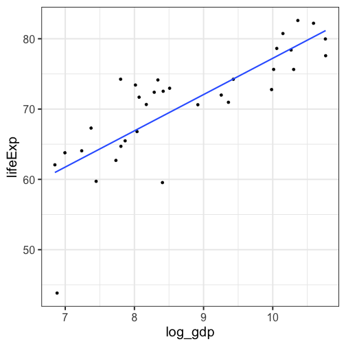<!-- --> --- ### Data, fitted, and residuals ```r library(broom) model_info = augment(fit.1) head(model_info) ``` ``` ## # A tibble: 6 × 8 ## lifeExp log_gdp .fitted .resid .hat .sigma .cooksd .std.resid ## <dbl> <dbl> <dbl> <dbl> <dbl> <dbl> <dbl> <dbl> ## 1 43.8 6.88 61.1 -17.3 0.101 3.63 0.796 -3.76 ## 2 75.6 10.3 78.8 -3.15 0.0802 4.89 0.0199 -0.676 ## 3 64.1 7.24 63.0 1.08 0.0765 4.93 0.00224 0.233 ## 4 59.7 7.45 64.1 -4.33 0.0646 4.86 0.0294 -0.923 ## 5 73.0 8.51 69.5 3.43 0.0314 4.89 0.00836 0.718 ## 6 82.2 10.6 80.3 1.94 0.100 4.92 0.00994 0.422 ``` ```r describe(model_info, fast = T) ``` ``` ## vars n mean sd min max range se ## lifeExp 1 33 70.73 7.96 43.83 82.60 38.77 1.39 ## log_gdp 2 33 8.74 1.24 6.85 10.76 3.91 0.22 ## .fitted 3 33 70.73 6.37 60.98 81.16 20.19 1.11 ## .resid 4 33 0.00 4.77 -17.31 8.37 25.68 0.83 ## .hat 5 33 0.06 0.03 0.03 0.11 0.08 0.00 ## .sigma 6 33 4.84 0.23 3.63 4.93 1.30 0.04 ## .cooksd 7 33 0.04 0.14 0.00 0.80 0.80 0.02 ## .std.resid 8 33 0.00 1.02 -3.76 1.77 5.53 0.18 ``` ??? Point out the average of the residuals is 0, just like average deviation from the mean is 0. --- ### The relationship between `\(X_i\)` and `\(\hat{Y_i}\)` ```r model_info %>% ggplot(aes(x = log_gdp, y = .fitted)) + geom_point() + geom_smooth(se = F, method = "lm") + scale_x_continuous("X") + scale_y_continuous(expression(hat(Y))) + theme_bw(base_size = 30) ``` 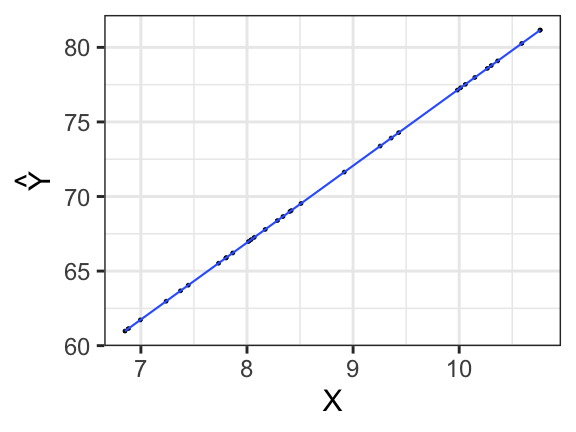<!-- --> --- ### The relationship between `\(X_i\)` and `\(e_i\)` ```r model_info %>% ggplot(aes(x = log_gdp, y = .resid)) + geom_point() + geom_smooth(se = F, method = "lm") + scale_x_continuous("X") + scale_y_continuous("e") + theme_bw(base_size = 30) ``` 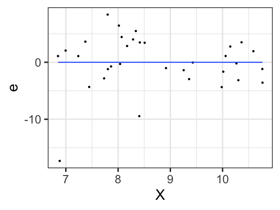<!-- --> --- ### The relationship between `\(Y_i\)` and `\(\hat{Y_i}\)` ```r model_info %>% ggplot(aes(x = lifeExp, y = .fitted)) + geom_point() + geom_smooth(se = F, method = "lm") + scale_x_continuous("Y") + scale_y_continuous(expression(hat(Y))) + theme_bw(base_size = 30) ``` 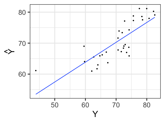<!-- --> --- ### The relationship between `\(Y_i\)` and `\(e_i\)` ```r model_info %>% ggplot(aes(x = lifeExp, y = .resid)) + geom_point() + geom_smooth(se = F, method = "lm") + scale_x_continuous("Y") + scale_y_continuous("e") + theme_bw(base_size = 25) ``` 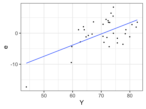<!-- --> --- ### The relationship between `\(\hat{Y_i}\)` and `\(e_i\)` ```r model_info %>% ggplot(aes(x = .fitted, y = .resid)) + geom_point() + geom_smooth(se = F, method = "lm") + scale_y_continuous("e") + scale_x_continuous(expression(hat(Y))) + theme_bw(base_size = 30) ``` 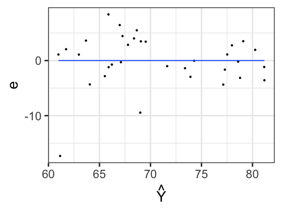<!-- --> --- ## Regression to the mean An observation about heights was part of the motivation to develop the regression equation: If you selected a parent who was exceptionally tall (or short), their child was almost always not as tall (or as short). 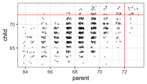<!-- --> --- ## Regression to the mean This phenomenon is known as **regression to the mean.** This describes the phenomenon in which an random variable produces an extreme score on a first measurement, but a lower score on a second measurement. .pull-left[ We can see this in the standardized regression equation: `$$\hat{Y_i} = r_{xy}(X_i) + e_i$$` In that the slope coefficient can never be greater than 1. ] .pull-right[  ] --- ## Regression to the mean This can be a threat to internal validity if interventions are applied based on first measurement scores. .pull-left[ <!-- --> ] -- .pull-right[ <!-- --> ] --- class: inverse ## Next time... Statistical inferences with regression