class: center, middle, inverse, title-slide # Partial correlations --- ## Annoucements * Homework due on Friday * No matrix algebra (enjoy with Elliot) --- ## Today - path diagrams - partial and semi-partial correlations --- ## Causal relationships Does parent socioeconomic status *cause* better grades? * `\(r_{\text{GPA},\text{SES}} = .33\)` -- Potential confound: Peer relationships - `\(r_{\text{SES}, \text{peer}} = .29\)` - `\(r_{\text{GPA}, \text{peer}} = .37\)` ??? Don't know how variables are related, only know that they are in a perfect world, we would want to **hold constant** peer relationships - control for - partial out --- ### Does parent SES cause better grades? 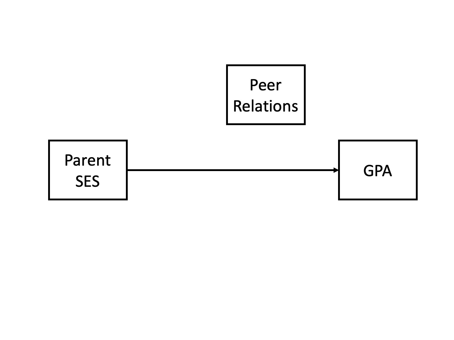 --- ### spurious relationship 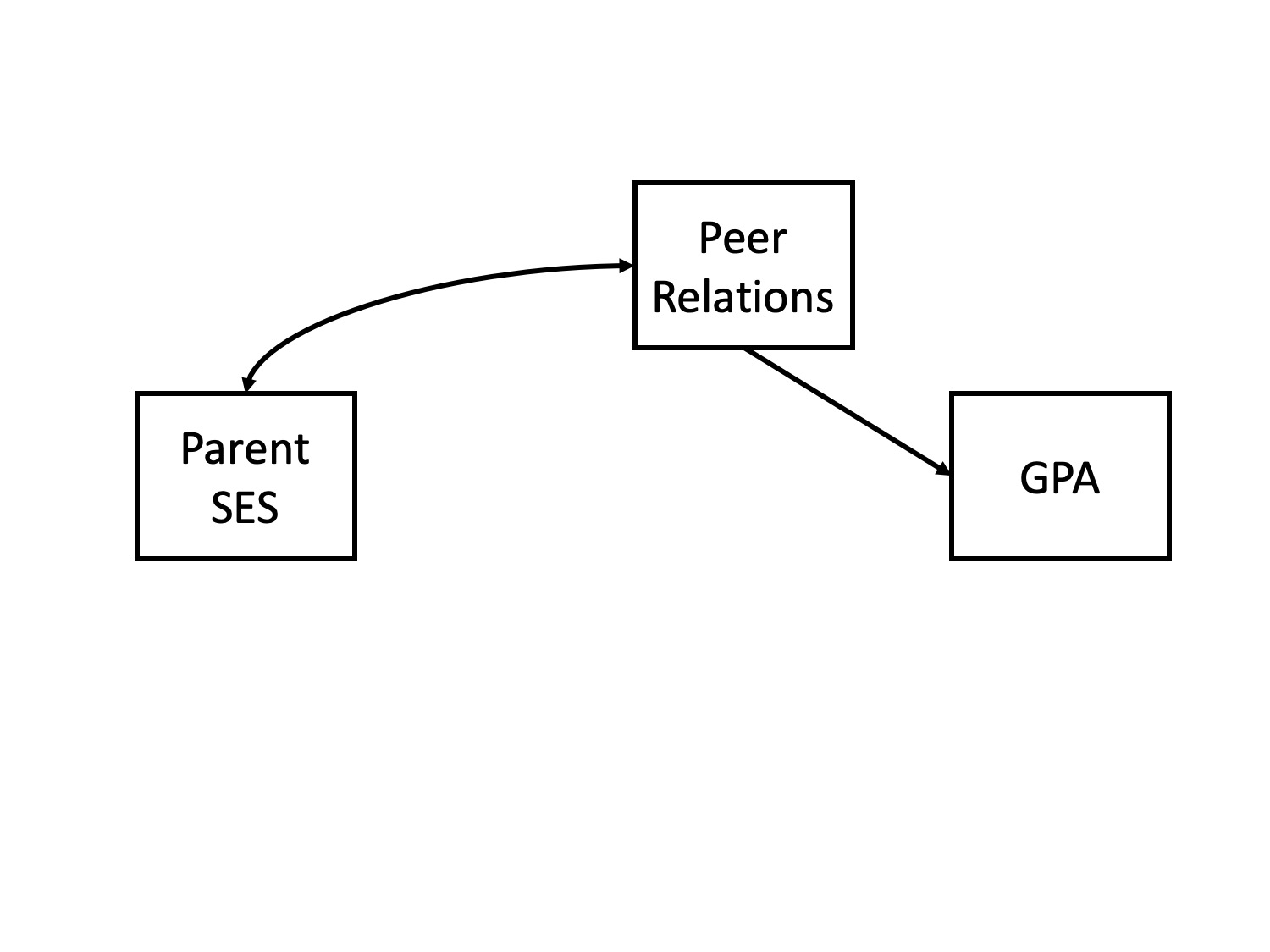 --- ### indirect (mediation) 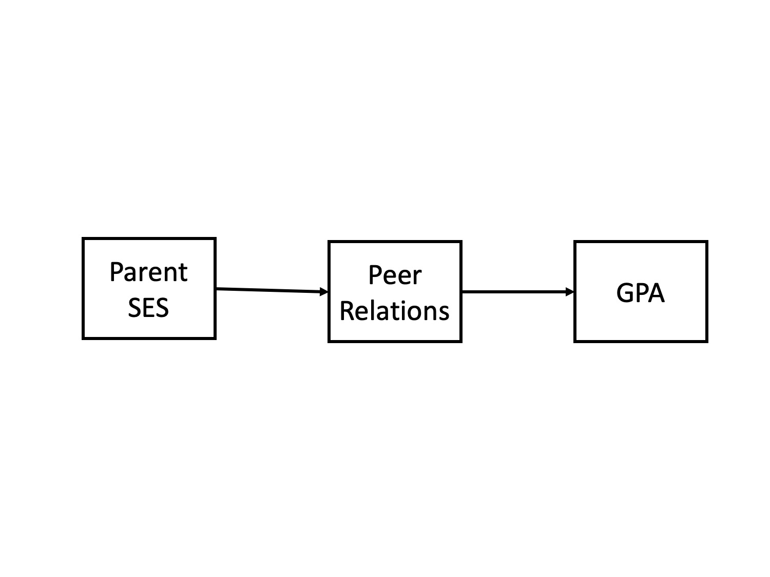 --- ### interaction (moderation) 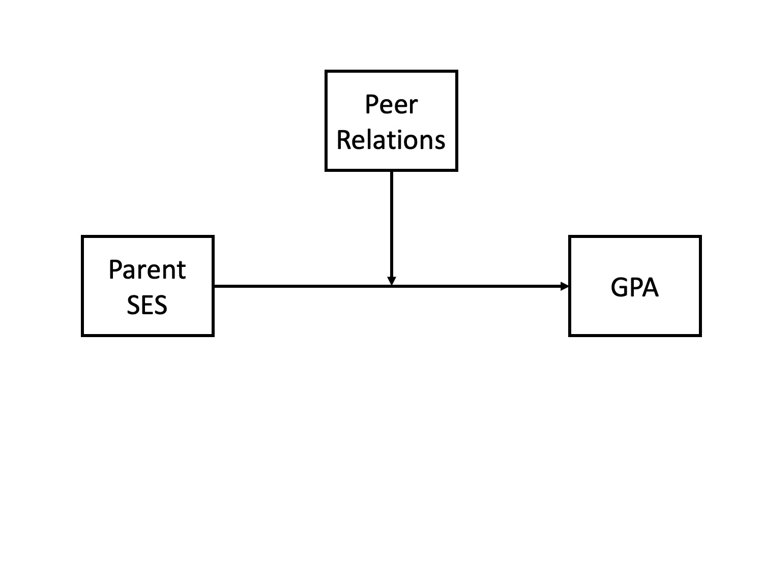 --- ### multiple causes 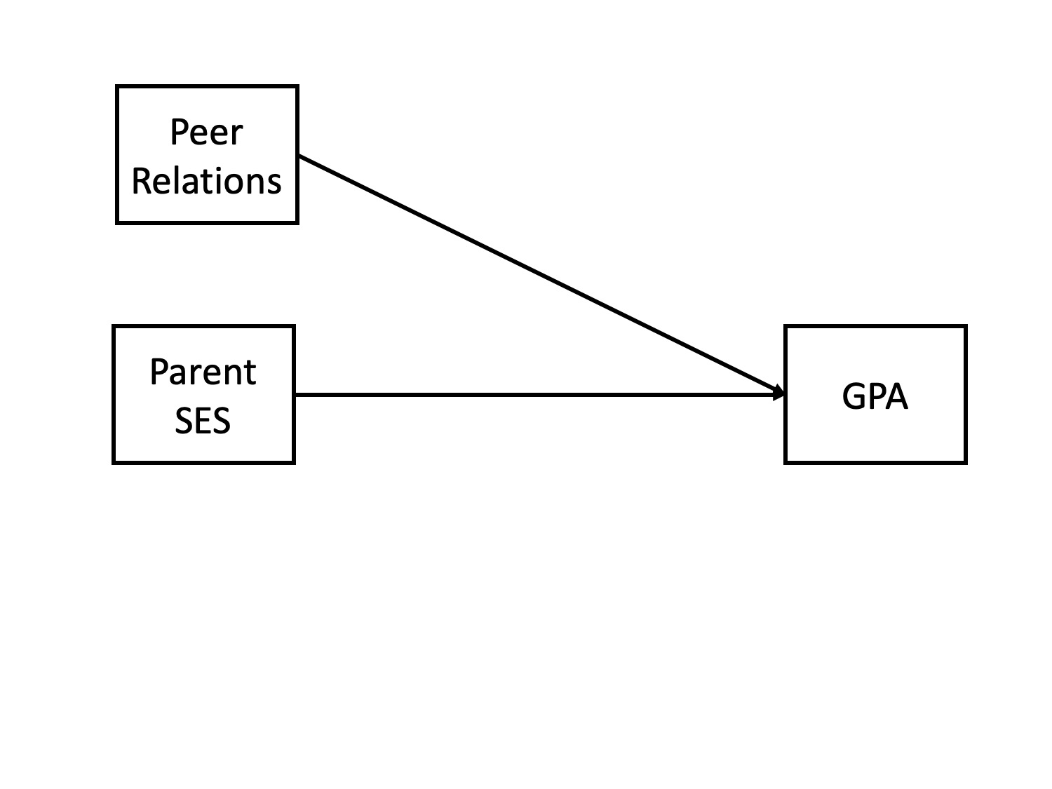 --- ### direct and indirect effects  --- ### multiple causes 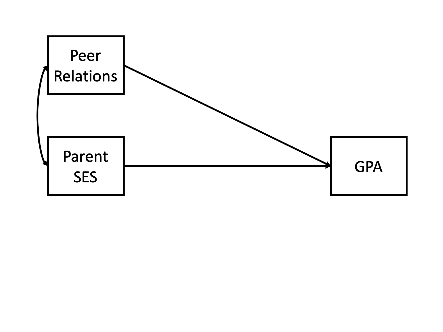 ??? This is the model implied by multiple regression models. --- ## General regression model `$$\large \hat{Y} = b_0 + b_1X_1 + b_2X_2 + \dots+b_kX_k$$` This is ultimately where we want to go. Unfortunately, it's not as simply as multiplying the correlation between Y and each X by the ratio of their standard errors and stringing them together. Why? --- ## What is `\(R^2\)`? .pull-left[ 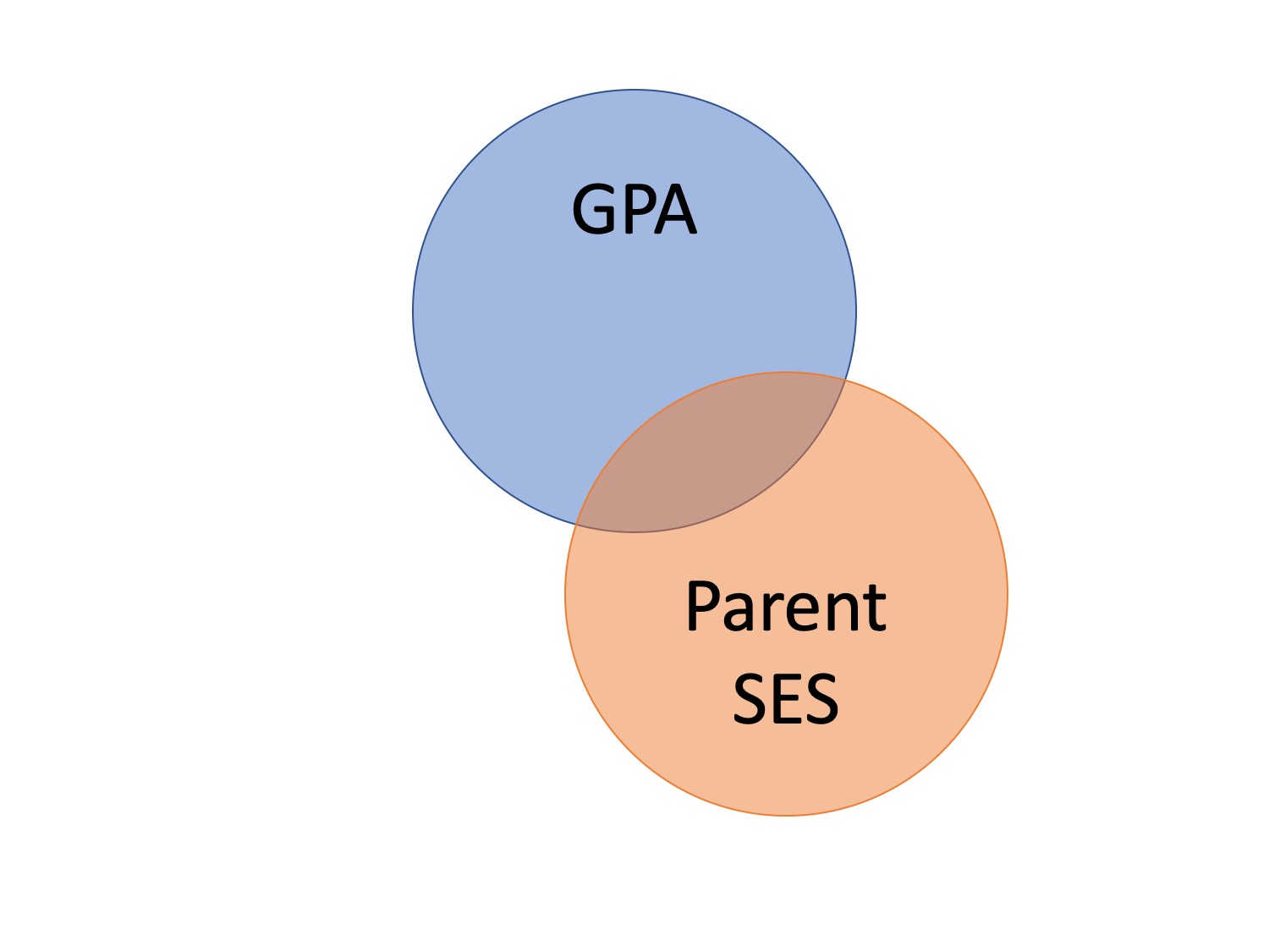 ] .pull-right[ `$$\large R^2 = \frac{s^2_{\hat{Y}}}{s^2_Y}$$` `$$\large = \frac{SS_{\text{Regression}}}{SS_Y}$$` ] --- 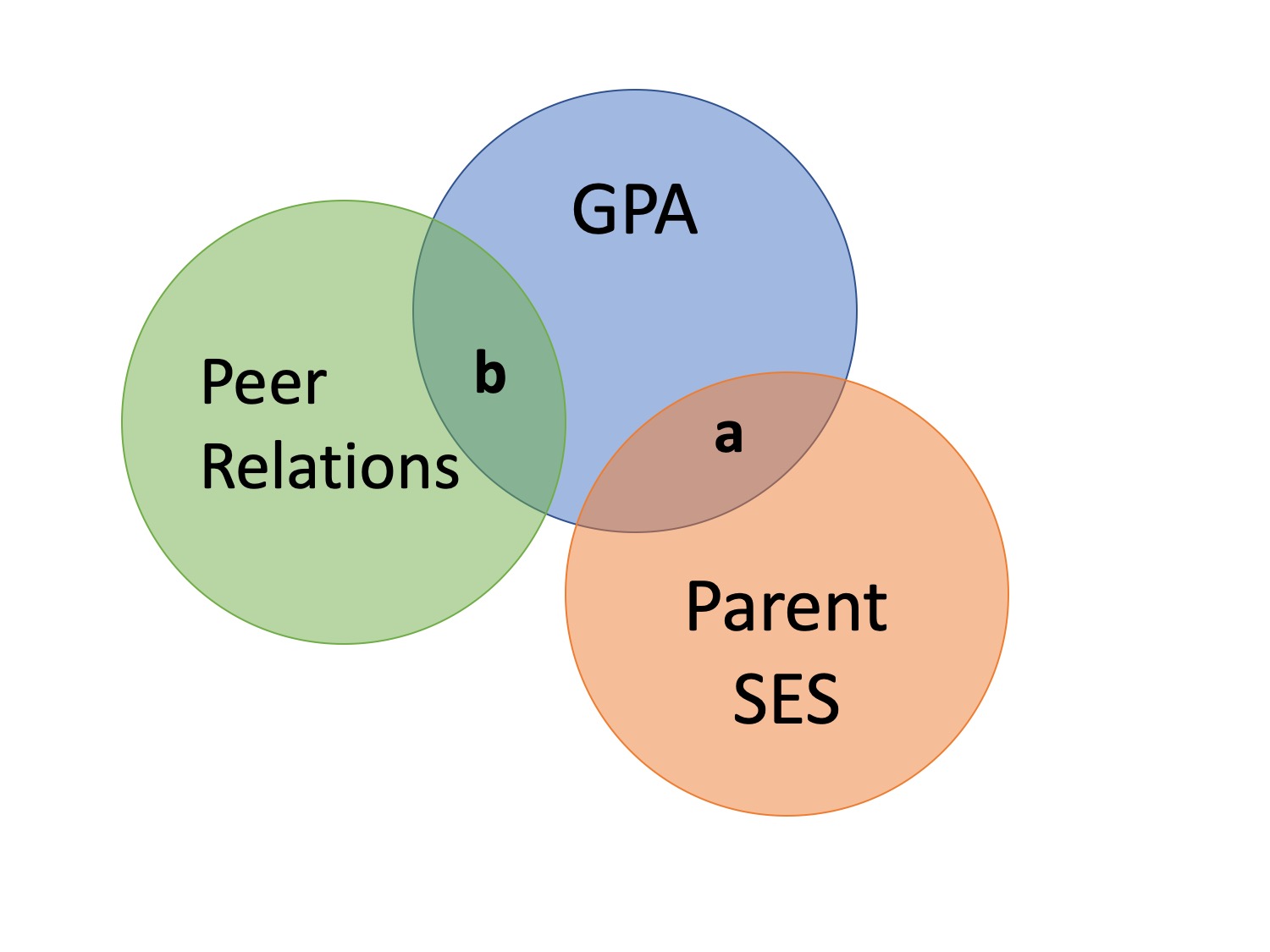 ### What is `\(R^2\)`? ---  ---  --- ### What is `\(R^2\)`? 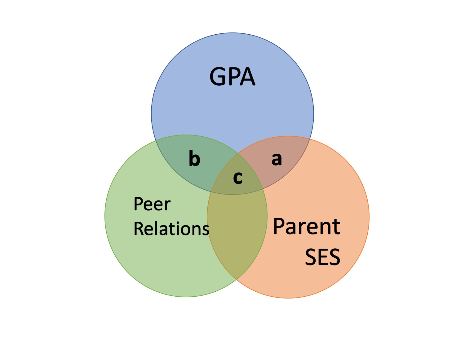 --- ### Types of correlations Pearson product moment correlation - Zero-order correlation - Only two variables are X and Y -- Semi-partial correlation - This correlation assess the extent to which the part of `\(X_1\)` *that is independent of* of `\(X_2\)` correlates with all of `\(Y\)` - This is often the estimate that we refer to when we talk about .purple[controlling for] another variable. --- 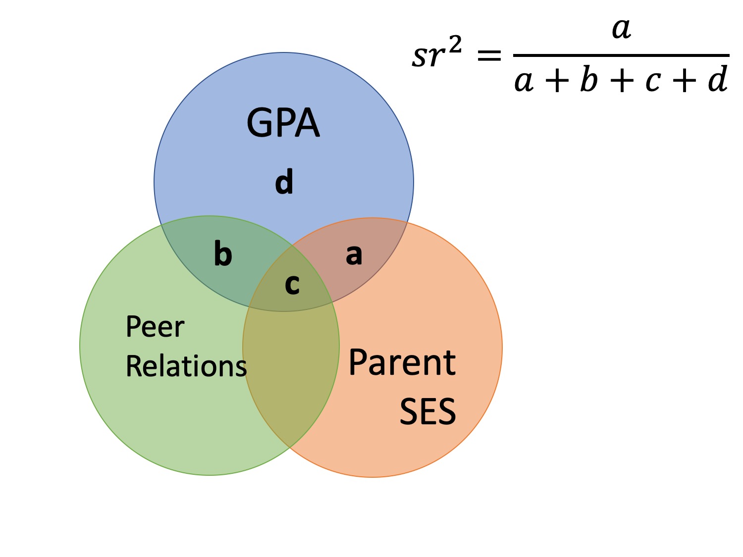 ??? the semi-partial correlation between parent SES and GPA controlling for peer relationships is a (not c), divided by all of GPA --- ### Semi-partial correlations `$$\large sr_1 = r_{Y(1.2)} = \frac{r_{Y1}-r_{Y2}r_{12}}{\sqrt{1-r^2_{12}}}$$` `$$\large sr_1^2 = R^2_{Y.12}-r^2_{Y2}$$` **Terms** `\(R_{Y.12}\)` -- The correlation of Y with the (best) linear combination of X1 and X2. `\(r_{Y(1.2)}\)` -- the semi-partial correlation of Y with X1 controlling for X2 --- ### Types of correlations Pearson product moment correlation - Zero-order correlation - Only two variables are X and Y Semi-partial correlation - This correlation assess the extent to which the part of `\(X_1\)` *that is independent of* of `\(X_2\)` correlates with all of Y - This is often the estimate that we refer to when we talk about **controlling for** another variable. -- Partial correlation - The extent to which the part of `\(X_1\)` that is independent of `\(X_2\)` is correlated with the part of `\(Y\)` that is also independent of `\(X_2\)`. --- 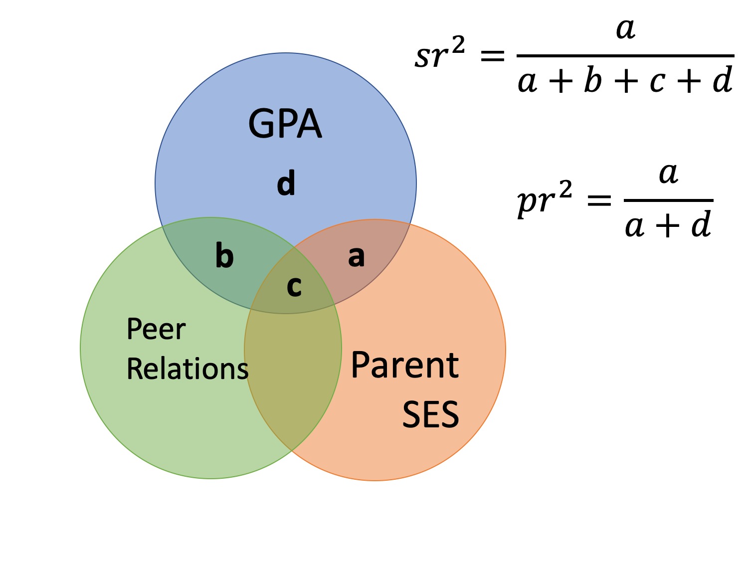 --- 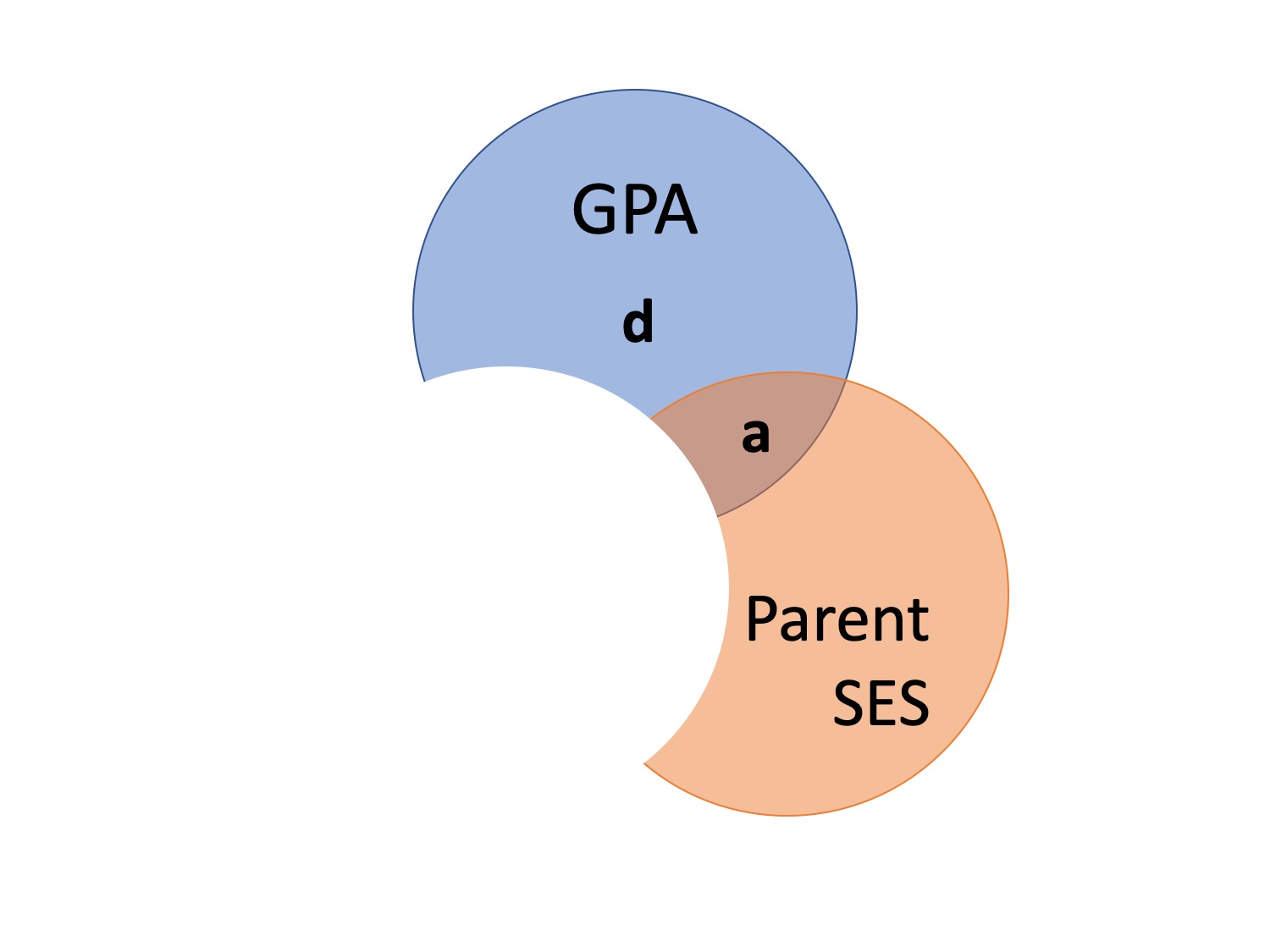 --- ### Partial correlations `$$\large pr_1=r_{Y1.2} = \frac{r_{Y1}-r_{Y2}r_{{12}}}{\sqrt{1-r^2_{Y2}}\sqrt{1-r^2_{12}}} = \frac{r_{Y(1.2)}}{\sqrt{1-r^2_{Y2}}}$$` **Terms** `\(R_{Y.12}\)` -- The correlation of Y with the (best) linear combination of X1 and X2. `\(r_{Y(1.2)}\)` -- the semi-partial correlation of Y with X1 controlling for X2 `\(r_{Y1.2}\)` -- the partial correlation of Y with X1 controlling for X2 --- ### What happens if `\(X_1\)` and `\(X_2\)` are uncorrelated? How does the semi-partial correlation compare to the zero-order correlation? -- `$$\large r_{Y(1.2)} = r_{Y1}$$` How does the partial correlation compare to the zero-order correlation? -- `$$\large r_{Y1.2} \neq r_{Y1}$$` --- ## When we use these? The semi-partial correlation is most often used when we want to show that some variable `\(Z\)` adds incremental variance in `\(Y\)` .purple[above and beyond] another `\(X\)` variable. - e.g., does nutrition predict Alzheimer's above and beyond known predictors like age, gender, and self-rated health? The partial correlations most often used when some .purple[third variable], `\(Z\)`, is a plausible explanation of the correlation between `\(X\)` and `\(Y\)` - e.g., can the relationship between ice cream and murder be explained by temperature? --- ## Example We'll use a dataset containing three variables: happiness, extraversion, and social support. There's some evidence that individuals high in extraversion experience more happiness. Is this because they receive more social support? If so, then the correlation between extraversion and happiness will be close to zero after accounting for social support. ```r library(here) data = read.csv(here("data/happy.csv")) ``` --- ```r data[,c("Extraversion", "Happiness", "SocSup")] %>% cor %>% round(3) ``` ``` ## Extraversion Happiness SocSup ## Extraversion 1.000 0.559 0.441 ## Happiness 0.559 1.000 0.445 ## SocSup 0.441 0.445 1.000 ``` The zero-order correlation between Happiness and Extraversion is 0.559 ```r library(ppcor) spcor.test(data$Happiness, # Y data$Extraversion, # X1 data$SocSup) # X2 ``` ``` ## estimate p.value statistic n gp Method ## 1 0.4040325 4.252627e-07 5.300267 147 1 pearson ``` The semi-partial correlation between Happiness and Extraversion is 0.404 --- ```r data[,c("Extraversion", "Happiness", "SocSup")] %>% cor %>% round(3) ``` ``` ## Extraversion Happiness SocSup ## Extraversion 1.000 0.559 0.441 ## Happiness 0.559 1.000 0.445 ## SocSup 0.441 0.445 1.000 ``` The zero-order correlation between Happiness and Extraversion is 0.559 ```r library(ppcor) pcor.test(data$Happiness, # Y data$Extraversion, # X1 data$SocSup) # X2 ``` ``` ## estimate p.value statistic n gp Method ## 1 0.4512658 1.087597e-08 6.068191 147 1 pearson ``` The partial correlation between Happiness and Extraversion is 0.451 --- ## `\(r_{(Y1.2)}\)` and `\(r_{Y1.2}\)` are correlations of residuals Recall that the residuals of a univariate regression equation are the part of the outcome `\((Y)\)` that is independent of the predictor `\((X)\)`. `$$\Large \hat{Y} = b_0 + b_1X$$` `$$\Large e_i = Y_i - \hat{Y_i}$$` We can use this to construct a measure of `\(X_1\)` that is independent of `\(X_2\)`: `$$\Large \hat{X}_{1.2} = b_0 + b_1X_2$$` `$$\Large e_{X_1} = X_1 - \hat{X}_{1.2}$$` --- We can either correlate that value with Y, to calculate our semi-partial correlation: `$$\Large r_{e_{X_1},Y} = r_{Y(1.2)}$$` Or we can calculate a measure of Y that is also independent of `\(X_2\)` and correlate that with our `\(X_1\)` residuals. `$$\Large \hat{Y} = b_0 + b_1X_2$$` `$$\Large e_{Y} = Y - \hat{Y}$$` `$$\Large r_{e_{X_1},e_{Y}} = r_{Y1.2}$$` --- ### Example ```r # create measure of happiness independent of social support mod.hap = lm(Happiness ~ SocSup, data = data) data.hap = broom::augment(mod.hap) # create measure of extraversion independent of social support mod.ext = lm(Extraversion ~ SocSup, data = data) data.ext = broom::augment(mod.ext) #semi-partial cor(data.ext$.resid, # residual of extraversion (X) data$Happiness) # original Happiness (Y) ``` ``` ## [1] 0.4040325 ``` ```r #partial cor(data.ext$.resid, # residual of extraversion (X) data.hap$.resid) # residual of Happiness (Y) ``` ``` ## [1] 0.4512658 ``` --- class: inverse ## Next time... Multiple regression!!