Psy 612: Data Analysis II

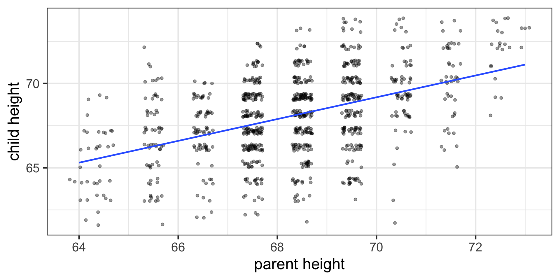
Scatter Plot with best fit line

Correlations
Univariate distributions
Code
pop = ggplot(data.frame(x = seq(-30, 30)), aes(x)) +
  stat_function(fun = function(x) dnorm(x, m = 0, sd = 10),
                geom = "area", fill = purples[3]) +
  scale_x_continuous("X") +
  scale_y_continuous("density", labels = NULL) +
  ggtitle("Population")+
  theme_bw(base_size = 20)
sample = data.frame(x = rnorm(n = 30, m = 0, sd = 10)) %>%
  ggplot(aes(x = x)) +
  geom_histogram(fill = purples[2], color = "black", bins = 20) +
  scale_x_continuous("X", limits = c(-30, 30)) +
  scale_y_continuous("frequency", labels = NULL) +
  ggtitle("Sample")+
  theme_bw(base_size = 20)
sampling = ggplot(data.frame(x = seq(-30, 30)), aes(x)) +
  stat_function(fun = function(x) dnorm(x, m = 0, sd = 10/sqrt(30)),
                geom = "area", fill = purples[3]) +
  scale_x_continuous("X") +
  scale_y_continuous("density", labels = NULL) +
  ggtitle("Sampling")+
  theme_bw(base_size = 20)

ggpubr::ggarrange(pop, sample, sampling)
Population
Code
mu1<-0 # setting the expected value of x1
mu2<-0 # setting the expected value of x2
s11<-4 # setting the variance of x1
s12<-2 # setting the covariance between x1 and x2
s22<-5 # setting the variance of x2
rho<-0.1 # setting the correlation coefficient between x1 and x2
x1<-seq(-10,10,length=41) # generating the vector series x1
x2<-x1 # copying x1 to x2
f<-function(x1,x2){
    term1<-1/(2*pi*sqrt(s11*s22*(1-rho^2)))
    term2<--1/(2*(1-rho^2))
    term3<-(x1-mu1)^2/s11
    term4<-(x2-mu2)^2/s22
    term5<--2*rho*((x1-mu1)*(x2-mu2))/(sqrt(s11)*sqrt(s22))
    term1*exp(term2*(term3+term4-term5))
} # setting up the function of the multivariate normal density
#
z<-outer(x1,x2,f) # calculating the density values
#
persp(x1, x2, z,
main="Joint Probability Distribution", sub=expression(italic(f)~(bold(x))==frac(1,2~pi~sqrt(sigma[11]~ sigma[22]~(1-rho^2)))~phantom(0)^bold(.)~exp~bgroup("{", list(-frac(1,2(1-rho^2)),
bgroup("[", frac((x[1]~-~mu[1])^2, sigma[11])~-~2~rho~frac(x[1]~-~mu[1], sqrt(sigma[11]))~ frac(x[2]~-~mu[2],sqrt(sigma[22]))~+~ frac((x[2]~-~mu[2])^2, sigma[22]),"]")),"}")),
col= purples[3],
theta=30, phi=20,
r=50,
d=0.1,
expand=0.5,
ltheta=90, lphi=180,
shade=0.75,
ticktype="detailed",
nticks=5)

# produces the 3-D plot
mtext(expression(list(mu[1]==0,mu[2]==0,sigma[11]==4,sigma[22]==5,sigma[12 ]==2,rho==0.1)), side=3)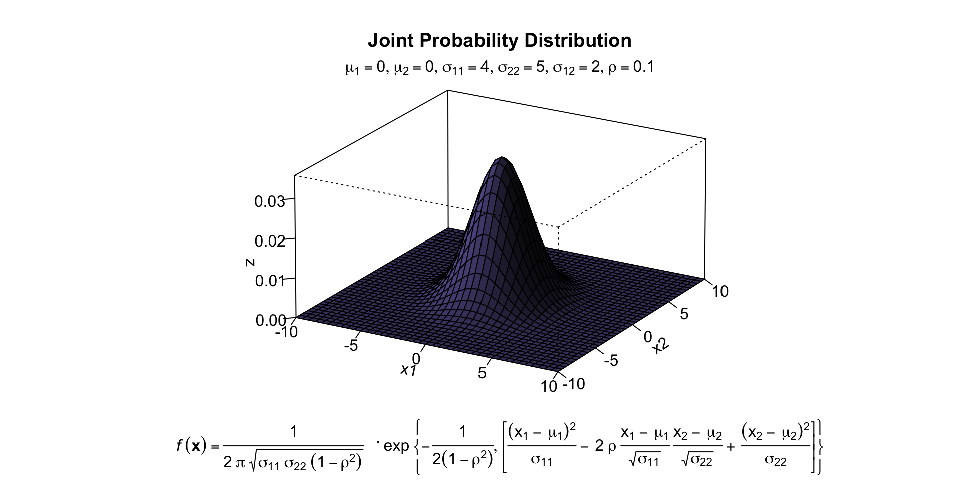
Sample
Code
sigma <- matrix( c( 4, 2,
                    2, 5 ), 2, 2 )  # covariance matrix

sample = BDgraph::rmvnorm(n = 30, mean = c(0,0), sigma = sigma)

sample %>% as.data.frame() %>%
  ggplot(aes(x = V1, y = V2)) +
  geom_smooth(method = "lm", se = F, color = purples[2])+
  geom_point(color = purples[3]) +
  scale_x_continuous("X1") +
  scale_y_continuous("X2")+
  theme_bw(base_size = 20)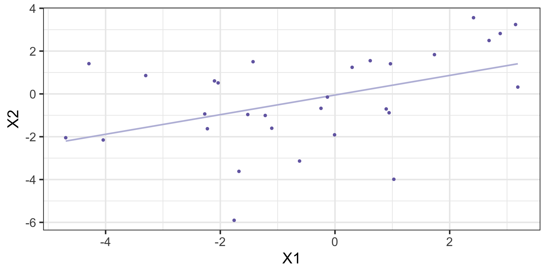
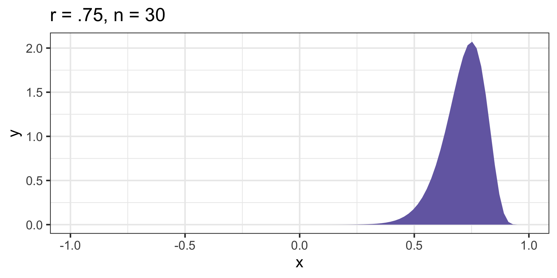
Skewed sampling distributions
Code
r_sampling = function(x, r, n){
  z = fisherz(r)
  se = 1/(sqrt(n-3))
  x_z = fisherz(x)
  density = dnorm(x_z, mean = z, sd = se)
  return(density)
}

cor_75 = ggplot(data.frame(x = seq(-.99, .99)), aes(x)) +
  stat_function(fun = function(x) r_sampling(x, r = .75,
                                             n = 30),
                geom = "area", fill = purples[3]) +
  scale_x_continuous(limits = c(-.99, .99)) +
  ggtitle("r = .75, n = 30") +
  theme_bw(base_size = 20)

cor_32 = ggplot(data.frame(x = seq(-.99, .99)), aes(x)) +
  stat_function(fun = function(x) r_sampling(x, r = .32,
                                             n = 30),
                geom = "area", fill = purples[2]) +
  scale_x_continuous(limits = c(-.99, .99)) +
  ggtitle("r = .32, n = 30")+
  theme_bw(base_size = 20)


cor_n85 = ggplot(data.frame(x = seq(-.99, .99)), aes(x)) +
  stat_function(fun = function(x) r_sampling(x, r = -.85,
                                             n = 30),
                geom = "area", fill = purples[3]) +
  scale_x_continuous(limits = c(-.99, .99)) +
  ggtitle("r = -.85, n = 30")+
  theme_bw(base_size = 20)

cor_75b = ggplot(data.frame(x = seq(-.99, .99)), aes(x)) +
  stat_function(fun = function(x) r_sampling(x, r = .75,
                                             n = 150),
                geom = "area", fill = purples[3]) +
  scale_x_continuous(limits = c(-.99, .99)) +
  ggtitle("r = .75, n = 150") +
  theme_bw(base_size = 20)

cor_32b = ggplot(data.frame(x = seq(-.99, .99)), aes(x)) +
  stat_function(fun = function(x) r_sampling(x, r = .32,
                                             n = 150),
                geom = "area", fill = purples[2]) +
  scale_x_continuous(limits = c(-.99, .99)) +
  ggtitle("r = .32, n = 150")+
  theme_bw(base_size = 20)


cor_n85b = ggplot(data.frame(x = seq(-.99, .99)), aes(x)) +
  stat_function(fun = function(x) r_sampling(x, r = -.85,
                                             n = 150),
                geom = "area", fill = purples[3]) +
  scale_x_continuous(limits = c(-.99, .99)) +
  ggtitle("r = -.85, n = 150")+
  theme_bw(base_size = 20)


ggpubr::ggarrange(cor_n85, cor_32, cor_75,
                  cor_n85b, cor_32b, cor_75b)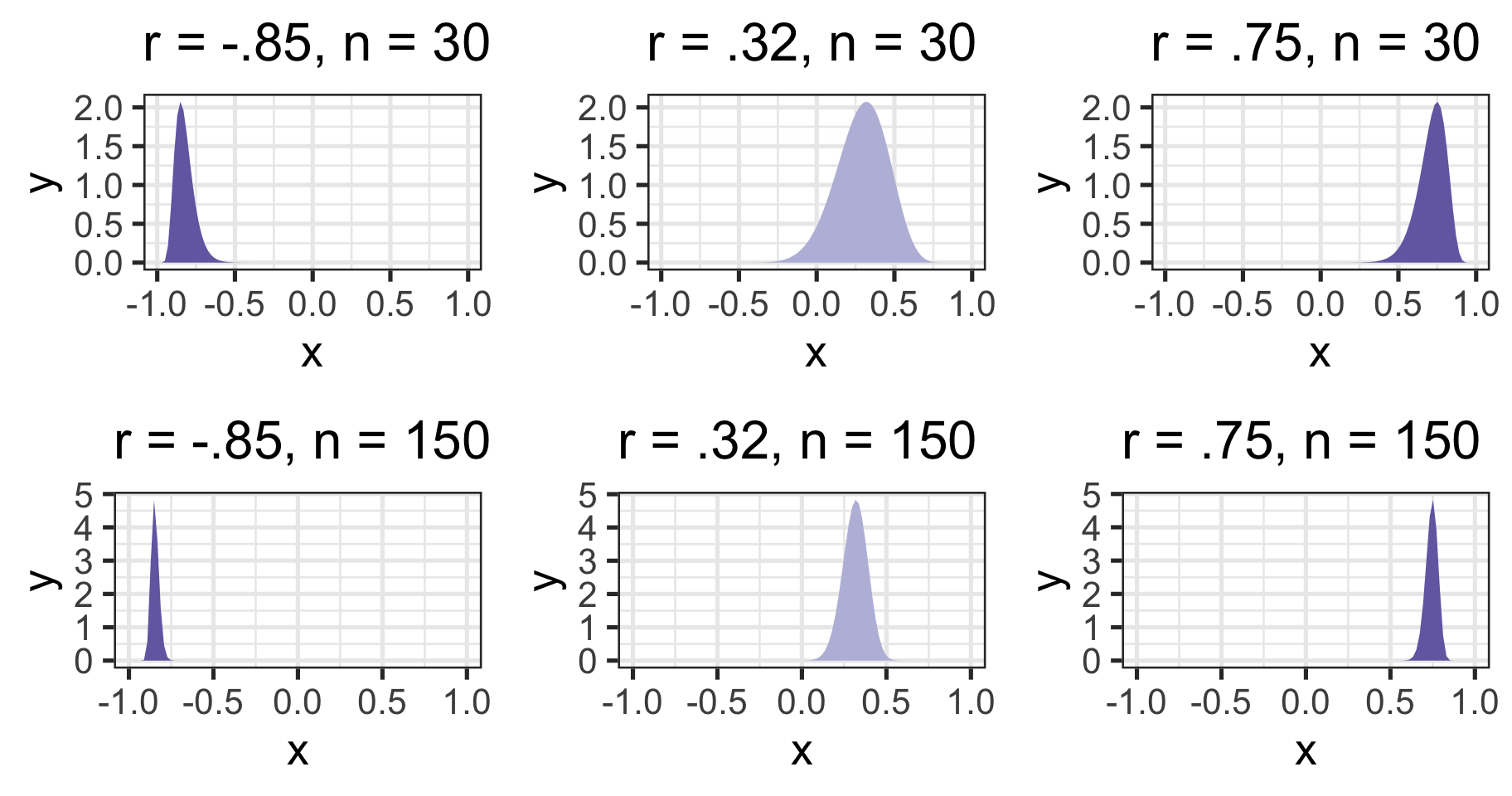
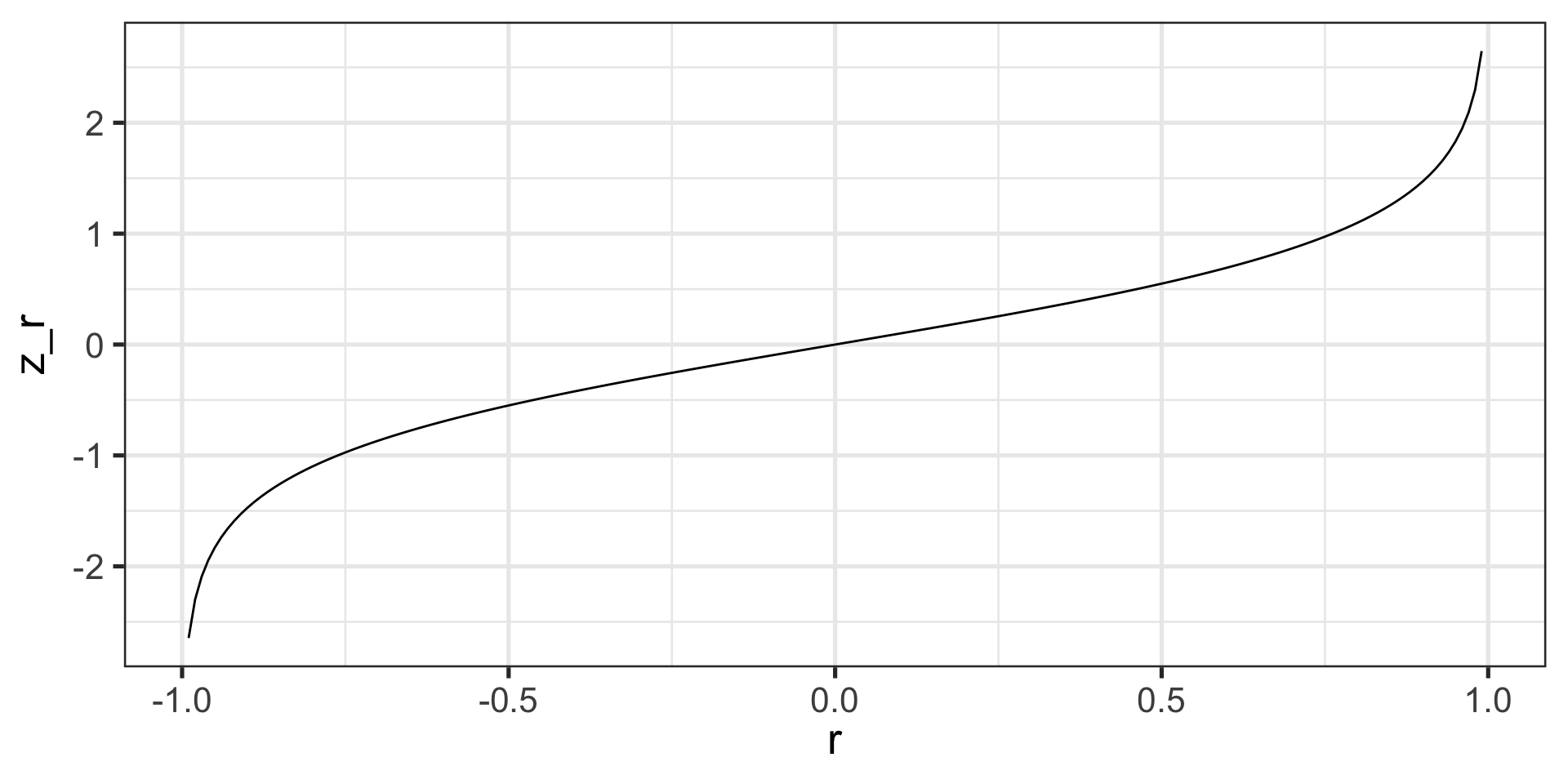
Fisher’s r to z’ transformation