Correlations
Part 2
Recap
Correlations are:
Standardized covariances
- Range from -1 to 1
an effect size
- Measure of the strength of association between two continuous variables
- Calculation:
- Sum the cross-product of deviation scores
- Divide by N-1
- Divide by the product of standard deviation scores
Example
Do Pulizters help newspapers keep readers? (Data from FiveThirtyEight).
            newspaper circ2004 circ2013 pctchg_circ num_finals1990_2003
1           USA Today  2192098  1674306         -24                   1
2 Wall Street Journal  2101017  2378827          13                  30
3      New York Times  1119027  1865318          67                  55
4   Los Angeles Times   983727   653868         -34                  44
5     Washington Post   760034   474767         -38                  52
6 New York Daily News   712671   516165         -28                   4
  num_finals2004_2014 num_finals1990_2014
1                   1                   2
2                  20                  50
3                  62                 117
4                  41                  85
5                  48                 100
6                   2                   6
x_var = pulitzer$pctchg_circ
y_var = pulitzer$num_finals2004_2014
n = length(x_var)
x_d = x_var - mean(x_var)
y_d = y_var - mean(y_var)
describe(cbind(x_var, x_d, y_var, y_d), fast = T) vars n mean sd min max range se
x_var 1 50 -29.20 27.07 -100.00 67.00 167 3.83
x_d 2 50 0.00 27.07 -70.80 96.20 167 3.83
y_var 3 50 6.72 12.14 0.00 62.00 62 1.72
y_d 4 50 0.00 12.14 -6.72 55.28 62 1.72 [1] -29.744 560.416 5317.936 -164.544 -363.264 -5.664 -48.384 -14.904
[9] -156.704 2.016 17.856 -4.464 126.496 36.816 -189.904 -146.624
[17] 25.456 -10.944 27.176 -25.024 14.336 3.976 3.776 116.416
[25] 65.536 404.976 -4.864 -7.224 -208.624 13.056 43.896 32.096
[33] 12.096 186.816 50.976 56.056 263.376 119.616 59.136 99.456
[41] -21.504 14.336 -61.824 -55.104 206.976 -46.784 40.176 99.456
[49] 40.176 -12.584[1] 6482.2[1] 132.2898[1] 0.4025279[1] 0.4025279
    Pearson's product-moment correlation

data:  pulitzer$pctchg_circ and pulitzer$num_finals2004_2014
t = 3.0465, df = 48, p-value = 0.003755
alternative hypothesis: true correlation is not equal to 0
95 percent confidence interval:
 0.1398493 0.6122747
sample estimates:
      cor
0.4025279
Note: cor.test cannot handle a null hypothesis other than 0. You’ll have to calculate significance by hand if you’re interested in using another null.
Recap: testing the significance of a correlation
If the null hypothesis is the nil hypothesis:
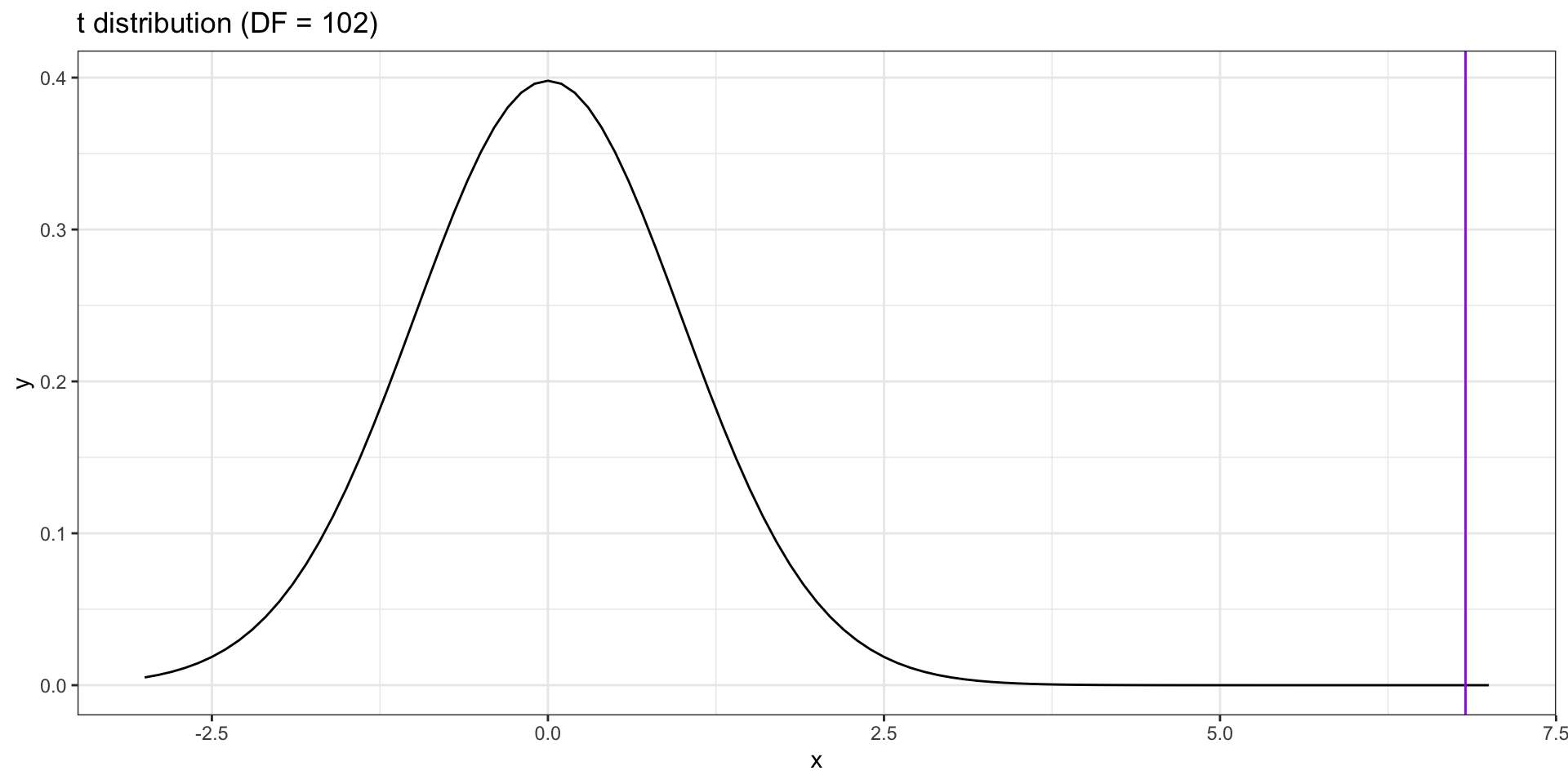
- test significance using a t-distribution, where
\[t = \frac{r}{SE_r}\] \[SE_r = \sqrt{\frac{1-r^2}{N-2}}\] \[DF = N-2\]
If null hypothesis is not 0 \((\text{e.g., }H_0:\rho_{xy} = .40)\)
- Transform statistic and null using Fisher’s r to Z
\[ z^{'} = {\frac{1}{2}}ln{\frac{1+r}{1-r}}\]
\[SE = \frac{1}{\sqrt{N-3}}\]
Example
In PSY 302, the correlation between midterm exam grades and final exam grades was .56. The class size was 104. Is this statistically significant?
Using t-method
\[SE_r = \sqrt{\frac{1-r^2}{N-2}} = \sqrt{\frac{1-.56^2}{104-2}} = 0.08\] \[t = \frac{r}{SE_r} = \frac{0.56}{0.08} = 6.83\]
Probability of getting a t statistic of 6.83 or greater is 0.
Example
In PSY 302, the correlation between midterm exam grades and final exam grades was .56. The class size was 104. Is this statistically significantly different from .40?
\[z^{'} = {\frac{1}{2}}ln{\frac{1+r}{1-r}}= {\frac{1}{2}}ln{\frac{1+0.56}{1-0.56}} = 0.63\] \[z^{'}_{H_0} = {\frac{1}{2}}ln{\frac{1+r}{1-r}}= {\frac{1}{2}}ln{\frac{1+0.4}{1-0.4}} = 0.42\] \[ SE_z = \frac{1}{\sqrt{104-3}} = 0.1\]
\[Z_{\text{statistic}} = \frac{z'-\mu}{SE_z}=\frac{0.63-0.42}{0.1} = 2.1\]
Today
- visualizing correlations
- correlation matrices
- reliability
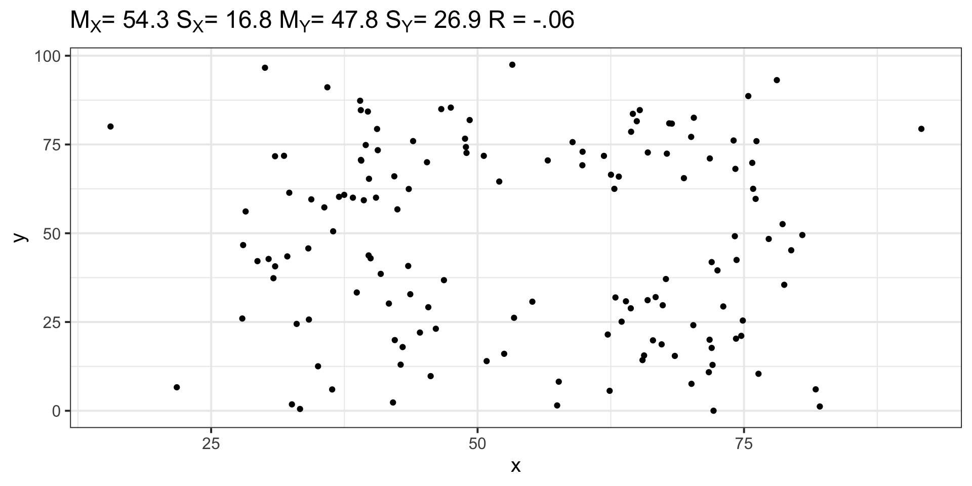
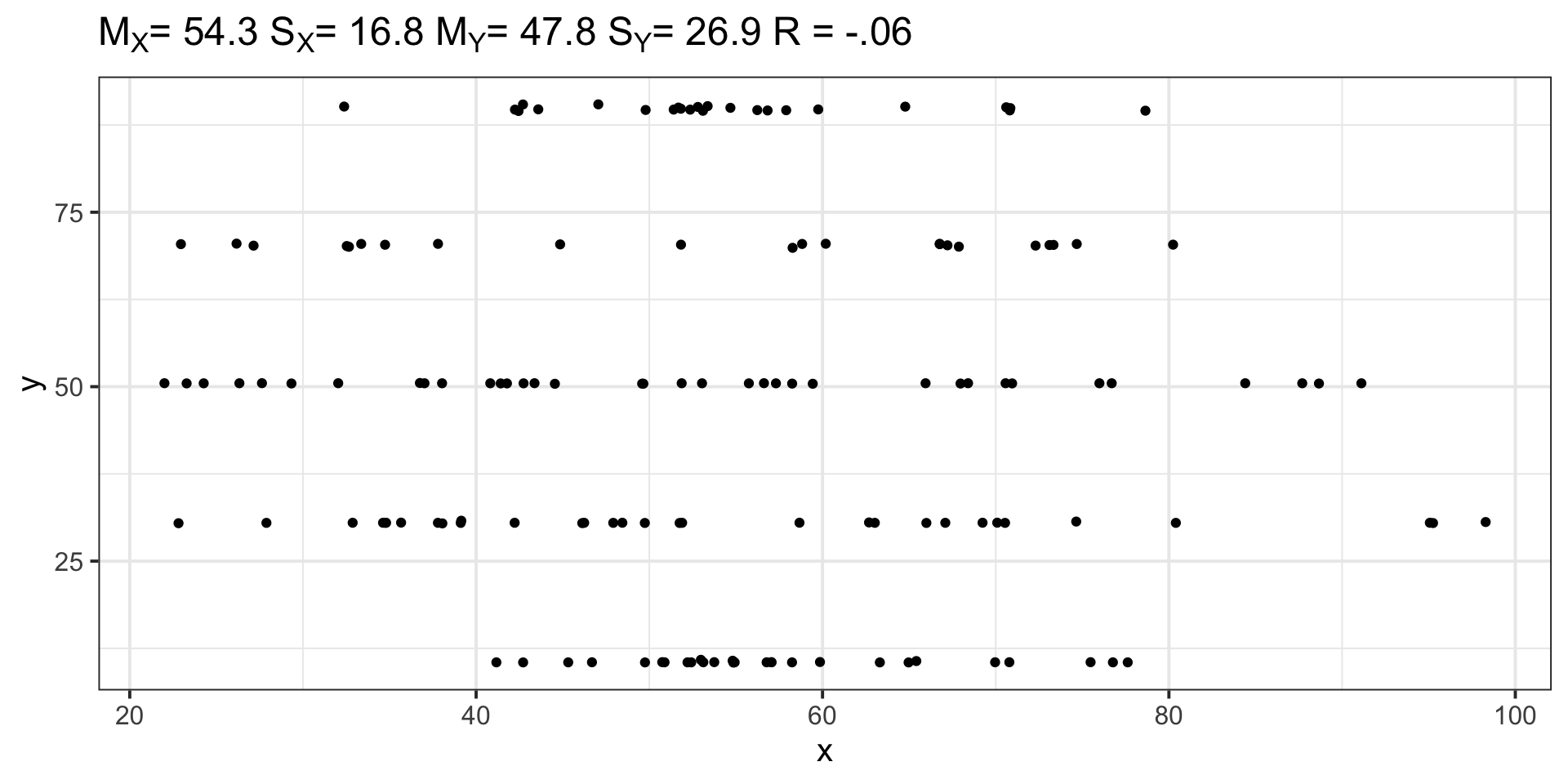
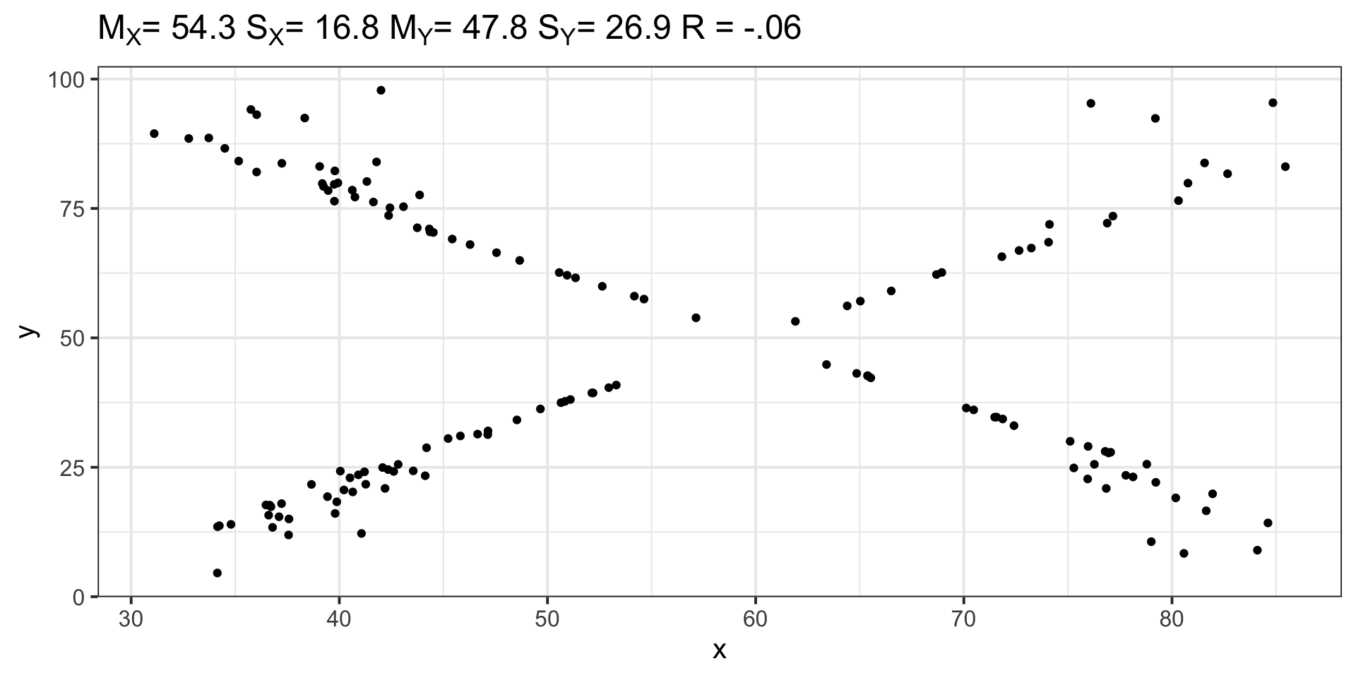
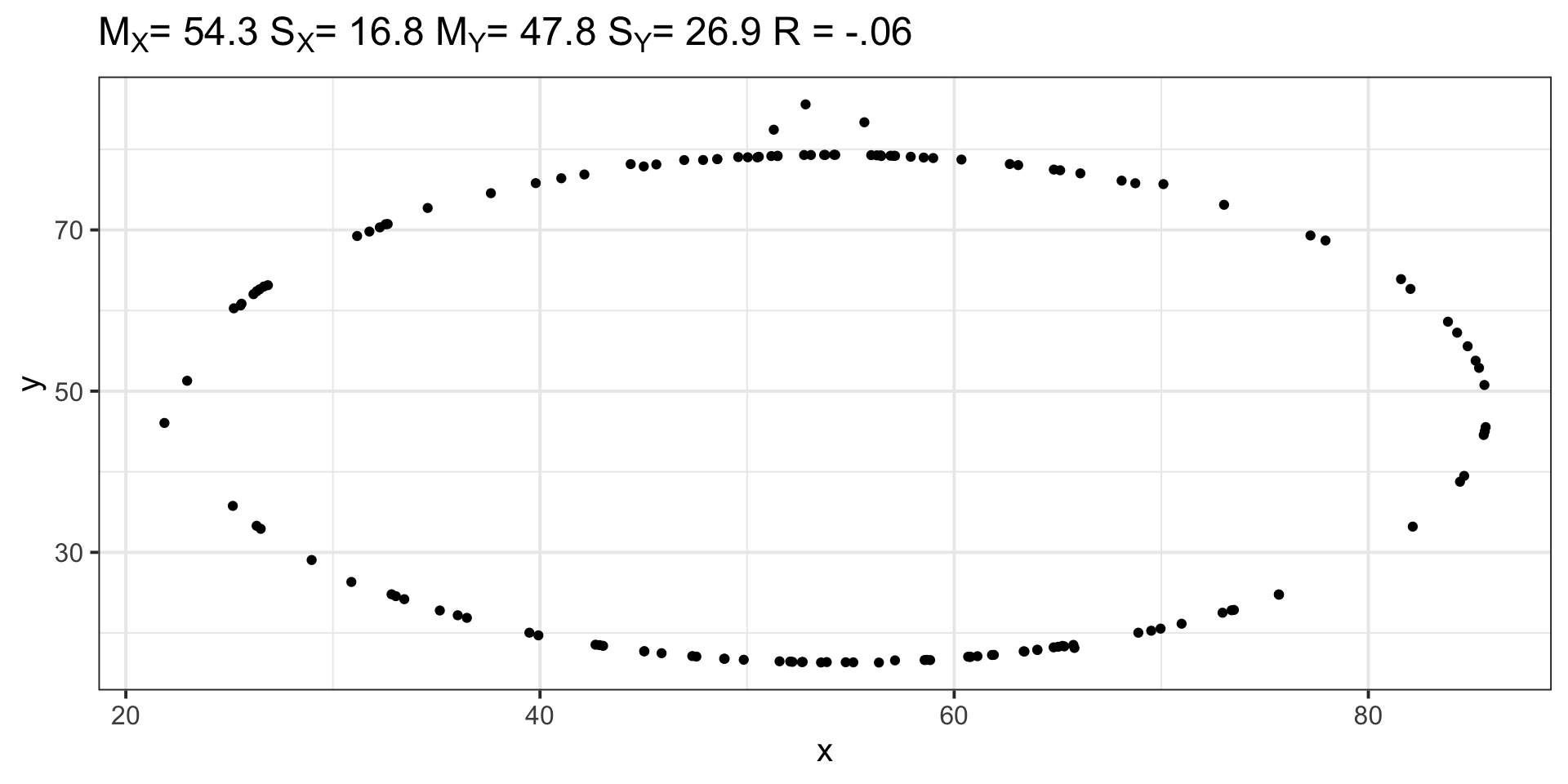
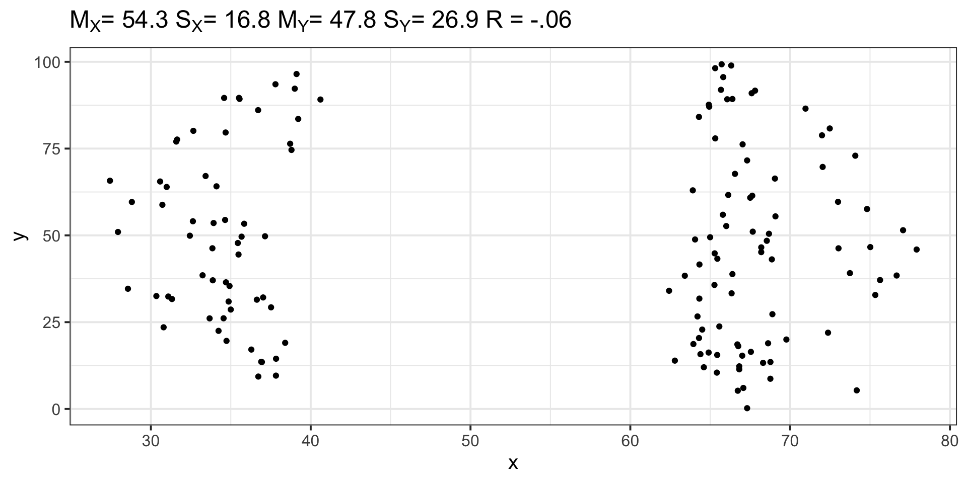
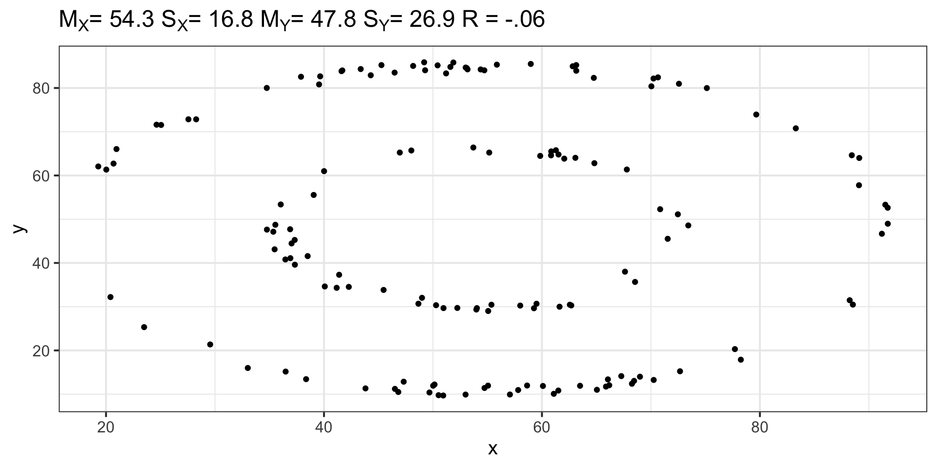
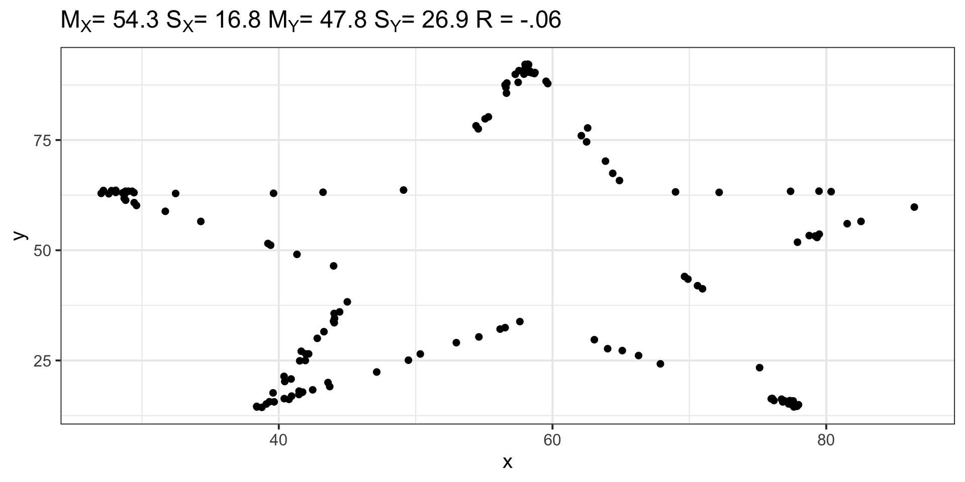
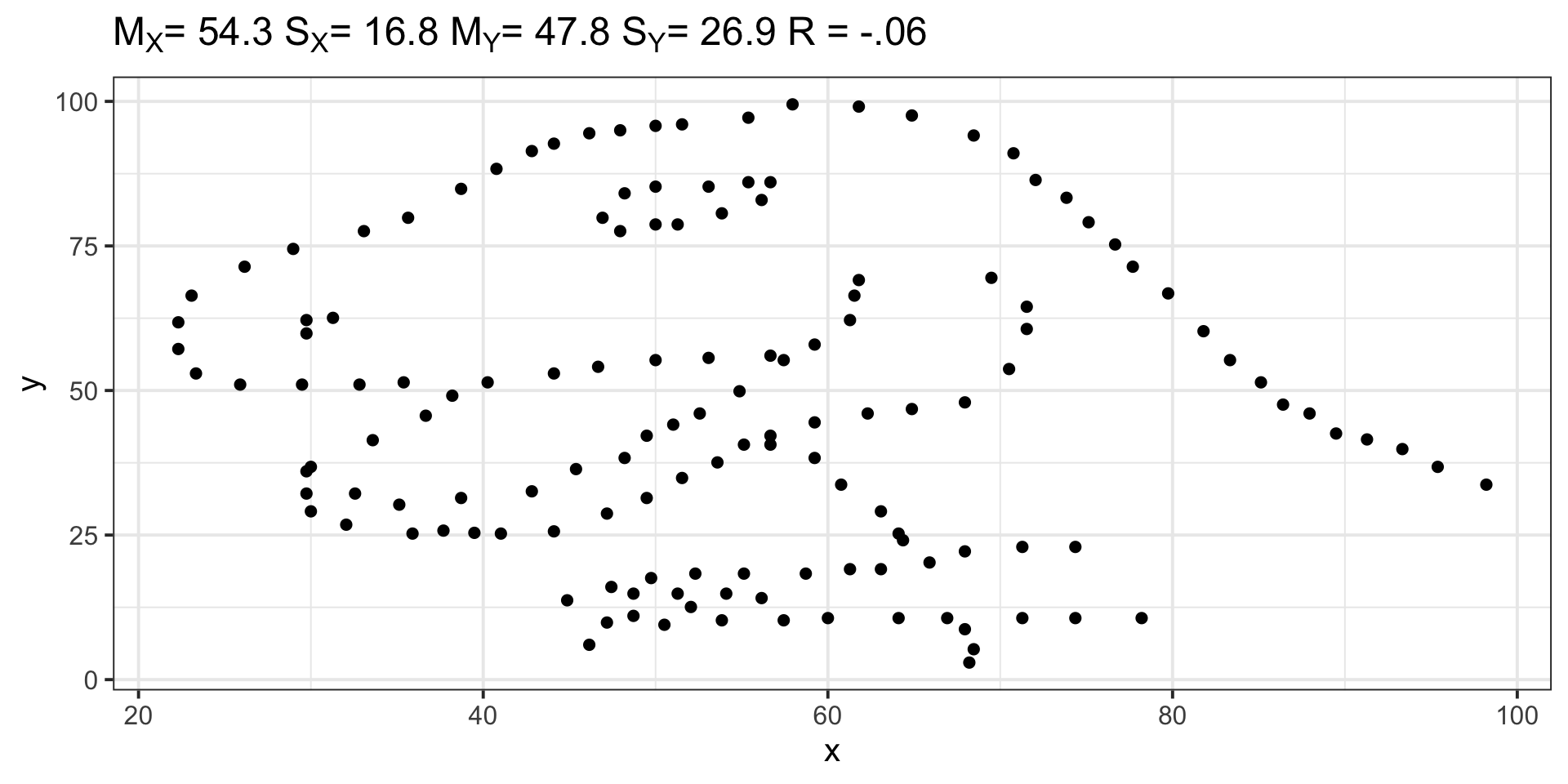
Visualizing correlations
For a single correlation, best practice is to visualize the relationship using a scatterplot. A best fit line is advised, as it can help clarify the strength and direction of the relationship.
Correlation matrices
Correlations are both a descriptive and an inferential statistic. As a descriptive statistic, they’re useful for understanding what’s going on in a larger dataset.
Like we use the summary() or describe() (psych) functions to examine our dataset before we run any infernetial tests, we should also look at the correlation matrix.
      A1 A2 A3 A4 A5 C1 C2 C3 C4 C5 E1 E2 E3 E4 E5 N1 N2 N3 N4 N5 O1 O2 O3 O4
61617  2  4  3  4  4  2  3  3  4  4  3  3  3  4  4  3  4  2  2  3  3  6  3  4
61618  2  4  5  2  5  5  4  4  3  4  1  1  6  4  3  3  3  3  5  5  4  2  4  3
61620  5  4  5  4  4  4  5  4  2  5  2  4  4  4  5  4  5  4  2  3  4  2  5  5
61621  4  4  6  5  5  4  4  3  5  5  5  3  4  4  4  2  5  2  4  1  3  3  4  3
61622  2  3  3  4  5  4  4  5  3  2  2  2  5  4  5  2  3  4  4  3  3  3  4  3
61623  6  6  5  6  5  6  6  6  1  3  2  1  6  5  6  3  5  2  2  3  4  3  5  6
      O5 gender education age
61617  3      1        NA  16
61618  3      2        NA  18
61620  2      2        NA  17
61621  5      2        NA  17
61622  3      1        NA  17
61623 1 2 3 21 A1 A2 A3 A4 A5 C1 C2 C3 C4 C5 E1 E2 E3 E4 E5 N1 N2 N3 N4 N5 O1
A1 1 NA NA NA NA NA NA NA NA NA NA NA NA NA NA NA NA NA NA NA NA
A2 NA 1 NA NA NA NA NA NA NA NA NA NA NA NA NA NA NA NA NA NA NA
A3 NA NA 1 NA NA NA NA NA NA NA NA NA NA NA NA NA NA NA NA NA NA
A4 NA NA NA 1 NA NA NA NA NA NA NA NA NA NA NA NA NA NA NA NA NA
A5 NA NA NA NA 1 NA NA NA NA NA NA NA NA NA NA NA NA NA NA NA NA
C1 NA NA NA NA NA 1 NA NA NA NA NA NA NA NA NA NA NA NA NA NA NA
C2 NA NA NA NA NA NA 1 NA NA NA NA NA NA NA NA NA NA NA NA NA NA
C3 NA NA NA NA NA NA NA 1 NA NA NA NA NA NA NA NA NA NA NA NA NA
C4 NA NA NA NA NA NA NA NA 1 NA NA NA NA NA NA NA NA NA NA NA NA
C5 NA NA NA NA NA NA NA NA NA 1 NA NA NA NA NA NA NA NA NA NA NA
E1 NA NA NA NA NA NA NA NA NA NA 1 NA NA NA NA NA NA NA NA NA NA
E2 NA NA NA NA NA NA NA NA NA NA NA 1 NA NA NA NA NA NA NA NA NA
E3 NA NA NA NA NA NA NA NA NA NA NA NA 1 NA NA NA NA NA NA NA NA
E4 NA NA NA NA NA NA NA NA NA NA NA NA NA 1 NA NA NA NA NA NA NA
E5 NA NA NA NA NA NA NA NA NA NA NA NA NA NA 1 NA NA NA NA NA NA
N1 NA NA NA NA NA NA NA NA NA NA NA NA NA NA NA 1 NA NA NA NA NA
N2 NA NA NA NA NA NA NA NA NA NA NA NA NA NA NA NA 1 NA NA NA NA
N3 NA NA NA NA NA NA NA NA NA NA NA NA NA NA NA NA NA 1 NA NA NA
N4 NA NA NA NA NA NA NA NA NA NA NA NA NA NA NA NA NA NA 1 NA NA
N5 NA NA NA NA NA NA NA NA NA NA NA NA NA NA NA NA NA NA NA 1 NA
O1 NA NA NA NA NA NA NA NA NA NA NA NA NA NA NA NA NA NA NA NA 1
O2 NA NA NA NA NA NA NA NA NA NA NA NA NA NA NA NA NA NA NA NA NA
O3 NA NA NA NA NA NA NA NA NA NA NA NA NA NA NA NA NA NA NA NA NA
O4 NA NA NA NA NA NA NA NA NA NA NA NA NA NA NA NA NA NA NA NA NA
O5 NA NA NA NA NA NA NA NA NA NA NA NA NA NA NA NA NA NA NA NA NA
gender NA NA NA NA NA NA NA NA NA NA NA NA NA NA NA NA NA NA NA NA NA
education NA NA NA NA NA NA NA NA NA NA NA NA NA NA NA NA NA NA NA NA NA
age NA NA NA NA NA NA NA NA NA NA NA NA NA NA NA NA NA NA NA NA NA
O2 O3 O4 O5 gender education age
A1 NA NA NA NA NA NA NA
A2 NA NA NA NA NA NA NA
A3 NA NA NA NA NA NA NA
A4 NA NA NA NA NA NA NA
A5 NA NA NA NA NA NA NA
C1 NA NA NA NA NA NA NA
C2 NA NA NA NA NA NA NA
C3 NA NA NA NA NA NA NA
C4 NA NA NA NA NA NA NA
C5 NA NA NA NA NA NA NA
E1 NA NA NA NA NA NA NA
E2 NA NA NA NA NA NA NA
E3 NA NA NA NA NA NA NA
E4 NA NA NA NA NA NA NA
E5 NA NA NA NA NA NA NA
N1 NA NA NA NA NA NA NA
N2 NA NA NA NA NA NA NA
N3 NA NA NA NA NA NA NA
N4 NA NA NA NA NA NA NA
N5 NA NA NA NA NA NA NA
O1 NA NA NA NA NA NA NA
O2 1.00000000 NA NA NA 0.02694778 NA -0.04254386
O3 NA 1 NA NA NA NA NA
O4 NA NA 1 NA NA NA NA
O5 NA NA NA 1 NA NA NA
gender 0.02694778 NA NA NA 1.00000000 NA 0.04770347
education NA NA NA NA NA 1 NA
age -0.04254386 NA NA NA 0.04770347 NA 1.00000000 A1 A2 A3 A4 A5 C1 C2 C3 C4 C5 E1
A1 1.00 -0.34 -0.27 -0.15 -0.18 0.03 0.02 -0.02 0.13 0.05 0.11
A2 -0.34 1.00 0.49 0.34 0.39 0.09 0.14 0.19 -0.15 -0.12 -0.21
A3 -0.27 0.49 1.00 0.36 0.50 0.10 0.14 0.13 -0.12 -0.16 -0.21
A4 -0.15 0.34 0.36 1.00 0.31 0.09 0.23 0.13 -0.15 -0.24 -0.11
A5 -0.18 0.39 0.50 0.31 1.00 0.12 0.11 0.13 -0.13 -0.17 -0.25
C1 0.03 0.09 0.10 0.09 0.12 1.00 0.43 0.31 -0.34 -0.25 -0.02
C2 0.02 0.14 0.14 0.23 0.11 0.43 1.00 0.36 -0.38 -0.30 0.02
C3 -0.02 0.19 0.13 0.13 0.13 0.31 0.36 1.00 -0.34 -0.34 0.00
C4 0.13 -0.15 -0.12 -0.15 -0.13 -0.34 -0.38 -0.34 1.00 0.48 0.09
C5 0.05 -0.12 -0.16 -0.24 -0.17 -0.25 -0.30 -0.34 0.48 1.00 0.06
E1 0.11 -0.21 -0.21 -0.11 -0.25 -0.02 0.02 0.00 0.09 0.06 1.00
E2 0.09 -0.23 -0.29 -0.19 -0.33 -0.09 -0.06 -0.08 0.20 0.26 0.47
E3 -0.05 0.25 0.39 0.19 0.42 0.12 0.15 0.09 -0.08 -0.16 -0.33
E4 -0.06 0.28 0.38 0.30 0.47 0.14 0.12 0.09 -0.11 -0.20 -0.42
E5 -0.02 0.29 0.25 0.16 0.27 0.25 0.25 0.21 -0.24 -0.23 -0.30
N1 0.17 -0.09 -0.08 -0.10 -0.20 -0.07 -0.02 -0.07 0.22 0.21 0.02
N2 0.14 -0.05 -0.09 -0.14 -0.19 -0.04 -0.01 -0.06 0.16 0.25 0.01
N3 0.10 -0.04 -0.04 -0.07 -0.14 -0.03 0.00 -0.07 0.21 0.24 0.05
N4 0.05 -0.09 -0.13 -0.17 -0.20 -0.10 -0.05 -0.11 0.26 0.34 0.23
N5 0.02 0.02 -0.04 -0.01 -0.08 -0.05 0.05 -0.01 0.20 0.17 0.05
O1 0.01 0.13 0.15 0.06 0.16 0.17 0.16 0.09 -0.09 -0.08 -0.10
O2 0.08 0.02 0.00 0.04 0.00 -0.11 -0.04 -0.03 0.21 0.14 0.04
O3 -0.06 0.16 0.22 0.07 0.24 0.19 0.19 0.06 -0.08 -0.08 -0.22
O4 -0.08 0.09 0.04 -0.04 0.02 0.11 0.06 0.02 0.05 0.14 0.08
O5 0.11 -0.09 -0.05 0.02 -0.05 -0.12 -0.05 -0.01 0.20 0.06 0.10
gender -0.16 0.18 0.14 0.13 0.10 0.01 0.07 0.05 -0.08 -0.09 -0.13
education -0.14 0.01 0.00 -0.02 0.01 0.03 0.00 0.05 -0.04 0.03 0.00
age -0.16 0.11 0.07 0.14 0.13 0.08 0.02 0.07 -0.15 -0.09 -0.03
E2 E3 E4 E5 N1 N2 N3 N4 N5 O1 O2
A1 0.09 -0.05 -0.06 -0.02 0.17 0.14 0.10 0.05 0.02 0.01 0.08
A2 -0.23 0.25 0.28 0.29 -0.09 -0.05 -0.04 -0.09 0.02 0.13 0.02
A3 -0.29 0.39 0.38 0.25 -0.08 -0.09 -0.04 -0.13 -0.04 0.15 0.00
A4 -0.19 0.19 0.30 0.16 -0.10 -0.14 -0.07 -0.17 -0.01 0.06 0.04
A5 -0.33 0.42 0.47 0.27 -0.20 -0.19 -0.14 -0.20 -0.08 0.16 0.00
C1 -0.09 0.12 0.14 0.25 -0.07 -0.04 -0.03 -0.10 -0.05 0.17 -0.11
C2 -0.06 0.15 0.12 0.25 -0.02 -0.01 0.00 -0.05 0.05 0.16 -0.04
C3 -0.08 0.09 0.09 0.21 -0.07 -0.06 -0.07 -0.11 -0.01 0.09 -0.03
C4 0.20 -0.08 -0.11 -0.24 0.22 0.16 0.21 0.26 0.20 -0.09 0.21
C5 0.26 -0.16 -0.20 -0.23 0.21 0.25 0.24 0.34 0.17 -0.08 0.14
E1 0.47 -0.33 -0.42 -0.30 0.02 0.01 0.05 0.23 0.05 -0.10 0.04
E2 1.00 -0.38 -0.51 -0.37 0.17 0.19 0.20 0.35 0.25 -0.16 0.08
E3 -0.38 1.00 0.42 0.38 -0.05 -0.07 -0.02 -0.15 -0.07 0.33 -0.07
E4 -0.51 0.42 1.00 0.32 -0.14 -0.14 -0.10 -0.29 -0.09 0.14 0.06
E5 -0.37 0.38 0.32 1.00 0.04 0.04 -0.06 -0.21 -0.13 0.30 -0.08
N1 0.17 -0.05 -0.14 0.04 1.00 0.71 0.56 0.40 0.38 -0.05 0.13
N2 0.19 -0.07 -0.14 0.04 0.71 1.00 0.55 0.39 0.35 -0.05 0.13
N3 0.20 -0.02 -0.10 -0.06 0.56 0.55 1.00 0.52 0.43 -0.03 0.11
N4 0.35 -0.15 -0.29 -0.21 0.40 0.39 0.52 1.00 0.40 -0.05 0.08
N5 0.25 -0.07 -0.09 -0.13 0.38 0.35 0.43 0.40 1.00 -0.12 0.20
O1 -0.16 0.33 0.14 0.30 -0.05 -0.05 -0.03 -0.05 -0.12 1.00 -0.21
O2 0.08 -0.07 0.06 -0.08 0.13 0.13 0.11 0.08 0.20 -0.21 1.00
O3 -0.23 0.39 0.21 0.29 -0.05 -0.03 -0.03 -0.06 -0.08 0.40 -0.26
O4 0.17 0.05 -0.10 0.00 0.08 0.13 0.18 0.21 0.11 0.18 -0.07
O5 0.08 -0.11 0.05 -0.11 0.11 0.04 0.06 0.04 0.14 -0.24 0.32
gender -0.05 0.05 0.08 0.07 0.04 0.10 0.12 0.00 0.21 -0.10 0.03
education -0.01 0.00 -0.04 0.06 -0.05 -0.05 -0.05 0.01 -0.05 0.03 -0.09
age -0.11 0.00 -0.01 0.11 -0.09 -0.10 -0.11 -0.03 -0.10 0.05 -0.04
O3 O4 O5 gender education age
A1 -0.06 -0.08 0.11 -0.16 -0.14 -0.16
A2 0.16 0.09 -0.09 0.18 0.01 0.11
A3 0.22 0.04 -0.05 0.14 0.00 0.07
A4 0.07 -0.04 0.02 0.13 -0.02 0.14
A5 0.24 0.02 -0.05 0.10 0.01 0.13
C1 0.19 0.11 -0.12 0.01 0.03 0.08
C2 0.19 0.06 -0.05 0.07 0.00 0.02
C3 0.06 0.02 -0.01 0.05 0.05 0.07
C4 -0.08 0.05 0.20 -0.08 -0.04 -0.15
C5 -0.08 0.14 0.06 -0.09 0.03 -0.09
E1 -0.22 0.08 0.10 -0.13 0.00 -0.03
E2 -0.23 0.17 0.08 -0.05 -0.01 -0.11
E3 0.39 0.05 -0.11 0.05 0.00 0.00
E4 0.21 -0.10 0.05 0.08 -0.04 -0.01
E5 0.29 0.00 -0.11 0.07 0.06 0.11
N1 -0.05 0.08 0.11 0.04 -0.05 -0.09
N2 -0.03 0.13 0.04 0.10 -0.05 -0.10
N3 -0.03 0.18 0.06 0.12 -0.05 -0.11
N4 -0.06 0.21 0.04 0.00 0.01 -0.03
N5 -0.08 0.11 0.14 0.21 -0.05 -0.10
O1 0.40 0.18 -0.24 -0.10 0.03 0.05
O2 -0.26 -0.07 0.32 0.03 -0.09 -0.04
O3 1.00 0.19 -0.31 -0.04 0.09 0.04
O4 0.19 1.00 -0.18 0.00 0.05 0.01
O5 -0.31 -0.18 1.00 0.02 -0.06 -0.10
gender -0.04 0.00 0.02 1.00 0.01 0.05
education 0.09 0.05 -0.06 0.01 1.00 0.24
age 0.04 0.01 -0.10 0.05 0.24 1.00 A1 A2 A3 A4 A5 C1 C2 C3 C4 C5 E1
A1 1.00 -0.34 -0.26 -0.14 -0.19 0.02 0.01 -0.01 0.10 0.02 0.12
A2 -0.34 1.00 0.48 0.34 0.38 0.09 0.13 0.19 -0.14 -0.11 -0.24
A3 -0.26 0.48 1.00 0.38 0.50 0.10 0.14 0.13 -0.12 -0.15 -0.22
A4 -0.14 0.34 0.38 1.00 0.32 0.08 0.22 0.13 -0.16 -0.24 -0.14
A5 -0.19 0.38 0.50 0.32 1.00 0.12 0.11 0.13 -0.12 -0.16 -0.25
C1 0.02 0.09 0.10 0.08 0.12 1.00 0.43 0.32 -0.35 -0.25 -0.03
C2 0.01 0.13 0.14 0.22 0.11 0.43 1.00 0.36 -0.38 -0.30 0.02
C3 -0.01 0.19 0.13 0.13 0.13 0.32 0.36 1.00 -0.35 -0.35 -0.02
C4 0.10 -0.14 -0.12 -0.16 -0.12 -0.35 -0.38 -0.35 1.00 0.48 0.10
C5 0.02 -0.11 -0.15 -0.24 -0.16 -0.25 -0.30 -0.35 0.48 1.00 0.07
E1 0.12 -0.24 -0.22 -0.14 -0.25 -0.03 0.02 -0.02 0.10 0.07 1.00
E2 0.08 -0.24 -0.29 -0.20 -0.33 -0.10 -0.07 -0.09 0.21 0.26 0.47
E3 -0.04 0.25 0.38 0.20 0.41 0.13 0.15 0.10 -0.09 -0.17 -0.33
E4 -0.07 0.30 0.39 0.33 0.48 0.14 0.12 0.10 -0.12 -0.21 -0.42
E5 -0.02 0.30 0.26 0.16 0.27 0.26 0.25 0.22 -0.23 -0.24 -0.31
N1 0.16 -0.08 -0.07 -0.09 -0.19 -0.06 -0.02 -0.08 0.21 0.21 0.01
N2 0.13 -0.04 -0.08 -0.15 -0.19 -0.03 0.00 -0.06 0.15 0.24 0.01
N3 0.09 -0.02 -0.03 -0.07 -0.13 -0.01 0.01 -0.07 0.20 0.23 0.05
N4 0.04 -0.09 -0.13 -0.16 -0.21 -0.09 -0.04 -0.13 0.28 0.35 0.23
N5 0.01 0.02 -0.04 0.00 -0.08 -0.05 0.05 -0.04 0.21 0.18 0.04
O1 0.00 0.11 0.14 0.04 0.15 0.18 0.16 0.09 -0.10 -0.09 -0.10
O2 0.07 0.03 0.03 0.05 0.00 -0.13 -0.05 -0.03 0.21 0.12 0.06
O3 -0.06 0.15 0.22 0.04 0.22 0.19 0.18 0.06 -0.07 -0.07 -0.21
O4 -0.09 0.05 0.02 -0.06 0.00 0.08 0.03 0.00 0.07 0.14 0.08
O5 0.11 -0.08 -0.04 0.04 -0.04 -0.13 -0.06 0.00 0.18 0.05 0.09
gender -0.17 0.21 0.16 0.13 0.11 0.00 0.06 0.04 -0.07 -0.09 -0.15
education -0.14 0.02 0.00 -0.02 0.02 0.04 0.01 0.06 -0.04 0.04 0.00
age -0.14 0.09 0.04 0.11 0.10 0.08 0.00 0.05 -0.12 -0.07 -0.03
E2 E3 E4 E5 N1 N2 N3 N4 N5 O1 O2
A1 0.08 -0.04 -0.07 -0.02 0.16 0.13 0.09 0.04 0.01 0.00 0.07
A2 -0.24 0.25 0.30 0.30 -0.08 -0.04 -0.02 -0.09 0.02 0.11 0.03
A3 -0.29 0.38 0.39 0.26 -0.07 -0.08 -0.03 -0.13 -0.04 0.14 0.03
A4 -0.20 0.20 0.33 0.16 -0.09 -0.15 -0.07 -0.16 0.00 0.04 0.05
A5 -0.33 0.41 0.48 0.27 -0.19 -0.19 -0.13 -0.21 -0.08 0.15 0.00
C1 -0.10 0.13 0.14 0.26 -0.06 -0.03 -0.01 -0.09 -0.05 0.18 -0.13
C2 -0.07 0.15 0.12 0.25 -0.02 0.00 0.01 -0.04 0.05 0.16 -0.05
C3 -0.09 0.10 0.10 0.22 -0.08 -0.06 -0.07 -0.13 -0.04 0.09 -0.03
C4 0.21 -0.09 -0.12 -0.23 0.21 0.15 0.20 0.28 0.21 -0.10 0.21
C5 0.26 -0.17 -0.21 -0.24 0.21 0.24 0.23 0.35 0.18 -0.09 0.12
E1 0.47 -0.33 -0.42 -0.31 0.01 0.01 0.05 0.23 0.04 -0.10 0.06
E2 1.00 -0.40 -0.52 -0.39 0.17 0.20 0.19 0.35 0.26 -0.16 0.08
E3 -0.40 1.00 0.43 0.40 -0.04 -0.06 -0.01 -0.15 -0.09 0.33 -0.07
E4 -0.52 0.43 1.00 0.33 -0.14 -0.15 -0.13 -0.31 -0.09 0.12 0.05
E5 -0.39 0.40 0.33 1.00 0.04 0.05 -0.06 -0.21 -0.14 0.29 -0.09
N1 0.17 -0.04 -0.14 0.04 1.00 0.71 0.57 0.41 0.38 -0.05 0.14
N2 0.20 -0.06 -0.15 0.05 0.71 1.00 0.55 0.39 0.35 -0.05 0.12
N3 0.19 -0.01 -0.13 -0.06 0.57 0.55 1.00 0.52 0.43 -0.05 0.11
N4 0.35 -0.15 -0.31 -0.21 0.41 0.39 0.52 1.00 0.40 -0.06 0.08
N5 0.26 -0.09 -0.09 -0.14 0.38 0.35 0.43 0.40 1.00 -0.15 0.20
O1 -0.16 0.33 0.12 0.29 -0.05 -0.05 -0.05 -0.06 -0.15 1.00 -0.23
O2 0.08 -0.07 0.05 -0.09 0.14 0.12 0.11 0.08 0.20 -0.23 1.00
O3 -0.24 0.41 0.21 0.30 -0.03 -0.02 -0.03 -0.06 -0.08 0.39 -0.29
O4 0.17 0.04 -0.10 -0.02 0.09 0.13 0.17 0.23 0.11 0.17 -0.08
O5 0.08 -0.13 0.04 -0.11 0.10 0.02 0.05 0.03 0.14 -0.25 0.33
gender -0.08 0.05 0.11 0.08 0.04 0.09 0.11 -0.02 0.21 -0.11 0.04
education -0.01 0.01 -0.03 0.06 -0.04 -0.04 -0.04 0.01 -0.05 0.03 -0.10
age -0.10 -0.02 -0.01 0.10 -0.07 -0.09 -0.11 -0.02 -0.10 0.05 -0.04
O3 O4 O5 gender education age
A1 -0.06 -0.09 0.11 -0.17 -0.14 -0.14
A2 0.15 0.05 -0.08 0.21 0.02 0.09
A3 0.22 0.02 -0.04 0.16 0.00 0.04
A4 0.04 -0.06 0.04 0.13 -0.02 0.11
A5 0.22 0.00 -0.04 0.11 0.02 0.10
C1 0.19 0.08 -0.13 0.00 0.04 0.08
C2 0.18 0.03 -0.06 0.06 0.01 0.00
C3 0.06 0.00 0.00 0.04 0.06 0.05
C4 -0.07 0.07 0.18 -0.07 -0.04 -0.12
C5 -0.07 0.14 0.05 -0.09 0.04 -0.07
E1 -0.21 0.08 0.09 -0.15 0.00 -0.03
E2 -0.24 0.17 0.08 -0.08 -0.01 -0.10
E3 0.41 0.04 -0.13 0.05 0.01 -0.02
E4 0.21 -0.10 0.04 0.11 -0.03 -0.01
E5 0.30 -0.02 -0.11 0.08 0.06 0.10
N1 -0.03 0.09 0.10 0.04 -0.04 -0.07
N2 -0.02 0.13 0.02 0.09 -0.04 -0.09
N3 -0.03 0.17 0.05 0.11 -0.04 -0.11
N4 -0.06 0.23 0.03 -0.02 0.01 -0.02
N5 -0.08 0.11 0.14 0.21 -0.05 -0.10
O1 0.39 0.17 -0.25 -0.11 0.03 0.05
O2 -0.29 -0.08 0.33 0.04 -0.10 -0.04
O3 1.00 0.17 -0.32 -0.04 0.10 0.02
O4 0.17 1.00 -0.18 -0.04 0.06 0.00
O5 -0.32 -0.18 1.00 0.04 -0.06 -0.08
gender -0.04 -0.04 0.04 1.00 0.01 0.05
education 0.10 0.06 -0.06 0.01 1.00 0.25
age 0.02 0.00 -0.08 0.05 0.25 1.00With pairwise deletion, different sets of cases contribute to different correlations. That maximizes the sample sizes, but can lead to problems if the data are missing for some systematic reason.
Listwise deletion (often referred to in R as use complete cases) doesn’t have the same issue of biasing correlations, but does result in smaller samples and potentially limited generalizability.
A good practice is comparing the different matrices; if the correlation values are very different, this suggests that the missingness that affects pairwise deletion is systematic.
             A1    A2    A3    A4    A5    C1    C2    C3    C4    C5    E1
A1         0.00  0.00  0.00  0.00  0.00  0.01  0.00 -0.01  0.03  0.03 -0.01
A2         0.00  0.00  0.00 -0.01  0.01  0.00  0.01  0.01 -0.01 -0.01  0.03
A3         0.00  0.00  0.00 -0.02  0.00  0.00  0.00  0.00  0.00 -0.01  0.00
A4         0.00 -0.01 -0.02  0.00 -0.01  0.01  0.01  0.00  0.01  0.00  0.03
A5         0.00  0.01  0.00 -0.01  0.00  0.00  0.00  0.00 -0.01 -0.01  0.00
C1         0.01  0.00  0.00  0.01  0.00  0.00  0.00 -0.01  0.01  0.00  0.00
C2         0.00  0.01  0.00  0.01  0.00  0.00  0.00  0.00  0.00  0.00 -0.01
C3        -0.01  0.01  0.00  0.00  0.00 -0.01  0.00  0.00  0.02  0.01  0.02
C4         0.03 -0.01  0.00  0.01 -0.01  0.01  0.00  0.02  0.00 -0.01 -0.01
C5         0.03 -0.01 -0.01  0.00 -0.01  0.00  0.00  0.01 -0.01  0.00  0.00
E1        -0.01  0.03  0.00  0.03  0.00  0.00 -0.01  0.02 -0.01  0.00  0.00
E2         0.01  0.01  0.00  0.01  0.00  0.01  0.01  0.01 -0.01  0.00  0.00
E3         0.00  0.00  0.00 -0.01  0.00 -0.02  0.00 -0.02  0.01  0.01  0.01
E4         0.01 -0.02 -0.02 -0.03 -0.01  0.00  0.00 -0.01  0.01  0.01  0.00
E5         0.00  0.00 -0.01  0.00  0.00 -0.01  0.00  0.00  0.00  0.01  0.00
N1         0.01 -0.01 -0.02  0.00  0.00 -0.01  0.00  0.01  0.01  0.01  0.01
N2         0.01 -0.01  0.00  0.00  0.00 -0.01 -0.01  0.00  0.01  0.01  0.01
N3         0.01 -0.02 -0.01  0.00 -0.01 -0.02 -0.01  0.01  0.01  0.01  0.00
N4         0.01  0.00  0.00 -0.01  0.01 -0.01 -0.01  0.02 -0.02 -0.01  0.00
N5         0.01  0.00  0.00  0.00  0.00  0.00  0.00  0.02 -0.02 -0.01  0.01
O1         0.01  0.02  0.00  0.02  0.02 -0.01  0.01  0.00  0.01  0.01  0.00
O2         0.01 -0.02 -0.03 -0.01  0.00  0.02  0.01  0.00  0.00  0.02 -0.01
O3         0.00  0.02  0.01  0.03  0.02  0.00  0.01  0.01 -0.01 -0.01  0.00
O4         0.01  0.03  0.01  0.02  0.01  0.03  0.03  0.02 -0.02  0.00 -0.01
O5         0.01 -0.01 -0.01 -0.01 -0.01  0.01  0.00 -0.01  0.01  0.01  0.01
gender     0.01 -0.03 -0.02  0.00 -0.01  0.01  0.01  0.01 -0.01  0.00  0.02
education  0.00 -0.01 -0.01  0.00  0.00 -0.01 -0.01 -0.01  0.00 -0.01  0.00
age       -0.02  0.02  0.03  0.03  0.03  0.00  0.02  0.02 -0.03 -0.01  0.01
             E2    E3    E4    E5    N1    N2    N3    N4    N5    O1    O2
A1         0.01  0.00  0.01  0.00  0.01  0.01  0.01  0.01  0.01  0.01  0.01
A2         0.01  0.00 -0.02  0.00 -0.01 -0.01 -0.02  0.00  0.00  0.02 -0.02
A3         0.00  0.00 -0.02 -0.01 -0.02  0.00 -0.01  0.00  0.00  0.00 -0.03
A4         0.01 -0.01 -0.03  0.00  0.00  0.00  0.00 -0.01  0.00  0.02 -0.01
A5         0.00  0.00 -0.01  0.00  0.00  0.00 -0.01  0.01  0.00  0.02  0.00
C1         0.01 -0.02  0.00 -0.01 -0.01 -0.01 -0.02 -0.01  0.00 -0.01  0.02
C2         0.01  0.00  0.00  0.00  0.00 -0.01 -0.01 -0.01  0.00  0.01  0.01
C3         0.01 -0.02 -0.01  0.00  0.01  0.00  0.01  0.02  0.02  0.00  0.00
C4        -0.01  0.01  0.01  0.00  0.01  0.01  0.01 -0.02 -0.02  0.01  0.00
C5         0.00  0.01  0.01  0.01  0.01  0.01  0.01 -0.01 -0.01  0.01  0.02
E1         0.00  0.01  0.00  0.00  0.01  0.01  0.00  0.00  0.01  0.00 -0.01
E2         0.00  0.02  0.01  0.02  0.00  0.00  0.01 -0.01  0.00  0.00  0.00
E3         0.02  0.00 -0.01 -0.02 -0.01 -0.01 -0.01  0.01  0.01  0.00  0.01
E4         0.01 -0.01  0.00 -0.02  0.01  0.01  0.03  0.02  0.00  0.01  0.01
E5         0.02 -0.02 -0.02  0.00  0.00 -0.01  0.00  0.00  0.01  0.00  0.00
N1         0.00 -0.01  0.01  0.00  0.00  0.00 -0.01 -0.01 -0.01  0.00 -0.01
N2         0.00 -0.01  0.01 -0.01  0.00  0.00  0.00  0.00  0.00  0.00  0.00
N3         0.01 -0.01  0.03  0.00 -0.01  0.00  0.00  0.00  0.00  0.01  0.00
N4        -0.01  0.01  0.02  0.00 -0.01  0.00  0.00  0.00  0.00  0.01  0.00
N5         0.00  0.01  0.00  0.01 -0.01  0.00  0.00  0.00  0.00  0.03  0.00
O1         0.00  0.00  0.01  0.00  0.00  0.00  0.01  0.01  0.03  0.00  0.02
O2         0.00  0.01  0.01  0.00 -0.01  0.00  0.00  0.00  0.00  0.02  0.00
O3         0.02 -0.02  0.00  0.00 -0.02 -0.01  0.00  0.00  0.01  0.00  0.03
O4         0.00  0.01  0.01  0.01 -0.01  0.00  0.01 -0.02  0.01  0.01  0.01
O5         0.00  0.02  0.01  0.00  0.01  0.02  0.01  0.01 -0.01  0.01 -0.01
gender     0.02 -0.01 -0.03 -0.01  0.01  0.00  0.01  0.02  0.00  0.01 -0.02
education  0.00  0.00 -0.01  0.00  0.00 -0.01 -0.01  0.00 -0.01 -0.01  0.01
age        0.00  0.02  0.00  0.02 -0.01 -0.01  0.00 -0.01  0.00  0.00  0.00
             O3    O4    O5 gender education   age
A1         0.00  0.01  0.01   0.01      0.00 -0.02
A2         0.02  0.03 -0.01  -0.03     -0.01  0.02
A3         0.01  0.01 -0.01  -0.02     -0.01  0.03
A4         0.03  0.02 -0.01   0.00      0.00  0.03
A5         0.02  0.01 -0.01  -0.01      0.00  0.03
C1         0.00  0.03  0.01   0.01     -0.01  0.00
C2         0.01  0.03  0.00   0.01     -0.01  0.02
C3         0.01  0.02 -0.01   0.01     -0.01  0.02
C4        -0.01 -0.02  0.01  -0.01      0.00 -0.03
C5        -0.01  0.00  0.01   0.00     -0.01 -0.01
E1         0.00 -0.01  0.01   0.02      0.00  0.01
E2         0.02  0.00  0.00   0.02      0.00  0.00
E3        -0.02  0.01  0.02  -0.01      0.00  0.02
E4         0.00  0.01  0.01  -0.03     -0.01  0.00
E5         0.00  0.01  0.00  -0.01      0.00  0.02
N1        -0.02 -0.01  0.01   0.01      0.00 -0.01
N2        -0.01  0.00  0.02   0.00     -0.01 -0.01
N3         0.00  0.01  0.01   0.01     -0.01  0.00
N4         0.00 -0.02  0.01   0.02      0.00 -0.01
N5         0.01  0.01 -0.01   0.00     -0.01  0.00
O1         0.00  0.01  0.01   0.01     -0.01  0.00
O2         0.03  0.01 -0.01  -0.02      0.01  0.00
O3         0.00  0.02  0.01   0.01      0.00  0.01
O4         0.02  0.00  0.00   0.03     -0.01  0.01
O5         0.01  0.00  0.00  -0.01      0.00 -0.02
gender     0.01  0.03 -0.01   0.00      0.00  0.00
education  0.00 -0.01  0.00   0.00      0.00 -0.01
age        0.01  0.01 -0.02   0.00     -0.01  0.00
Types of missingness
Ideally our missingness is missing completely at random (MCAR). This means the probability of being missing is the same for all observations. If this is the case, our correlation estimates will be unbiased (if underpowered) and we’re free to use them with no concerns (other than the usual).
- Aliens beam into a warehouse and randomly take some files.
Types of missingness
However, our data might be missing at random (MAR). This means the probability of being missing is different between cases, and also the probability is related to variables we have observed. This is not great, but sometimes we can account for this using the variables we have observed (e.g., imputation, different estimation methods).
- Raccoons sneak into the warehouse and eat all the files by the door.
Types of missingness
It’s a problem if our data is missing not at random (MNAR). The probability of being missing differs for reasons that are unknown to us. This is especially problematic if the reason is associated with the variables at the heart of our study. Sensitivity analyses might help us detect MNAR-ness and possibly define the limits of our study, but we can’t adjust our data for this issue.
- Criminals break into the warehouse and steal files about themselves.
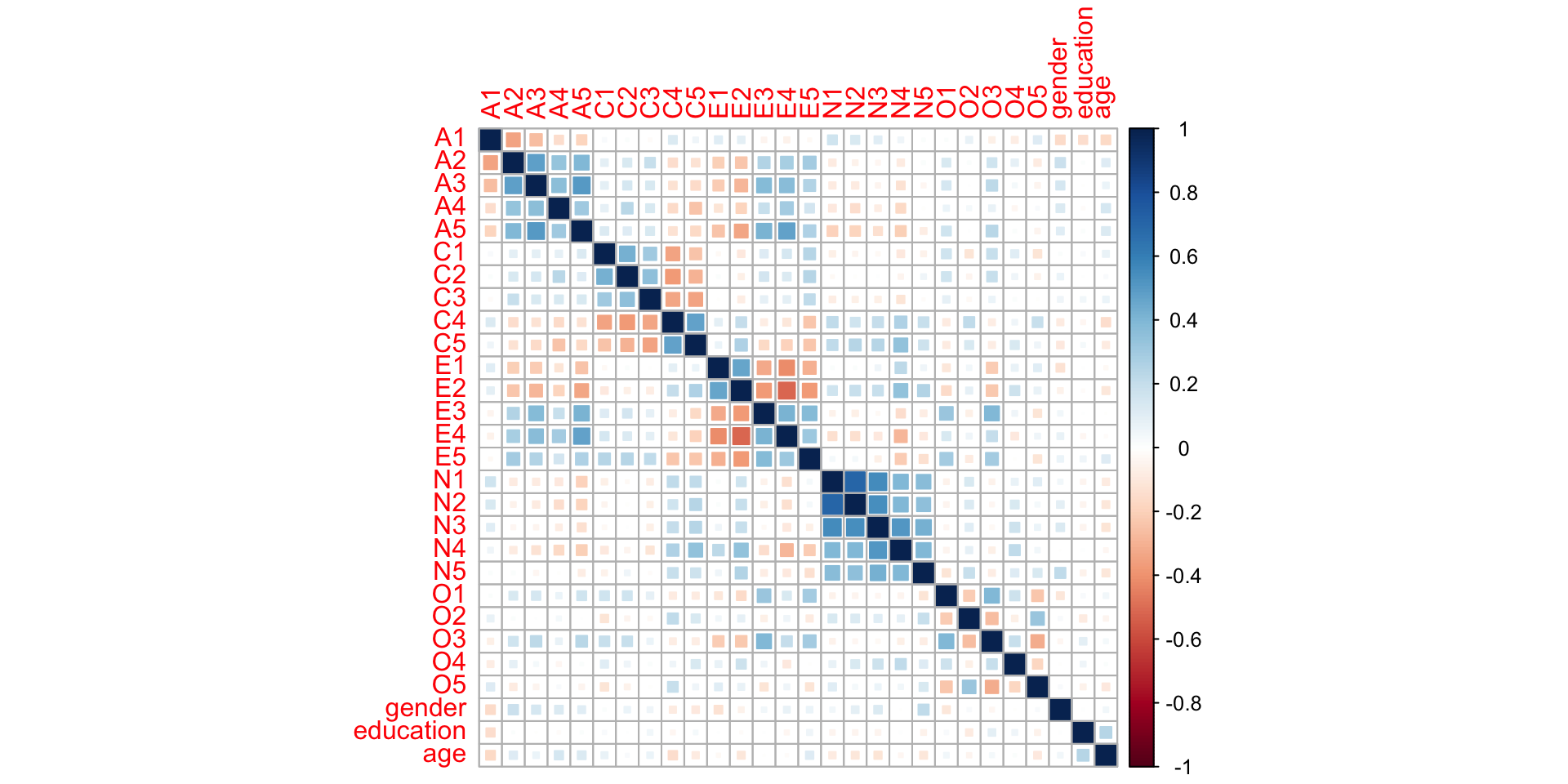
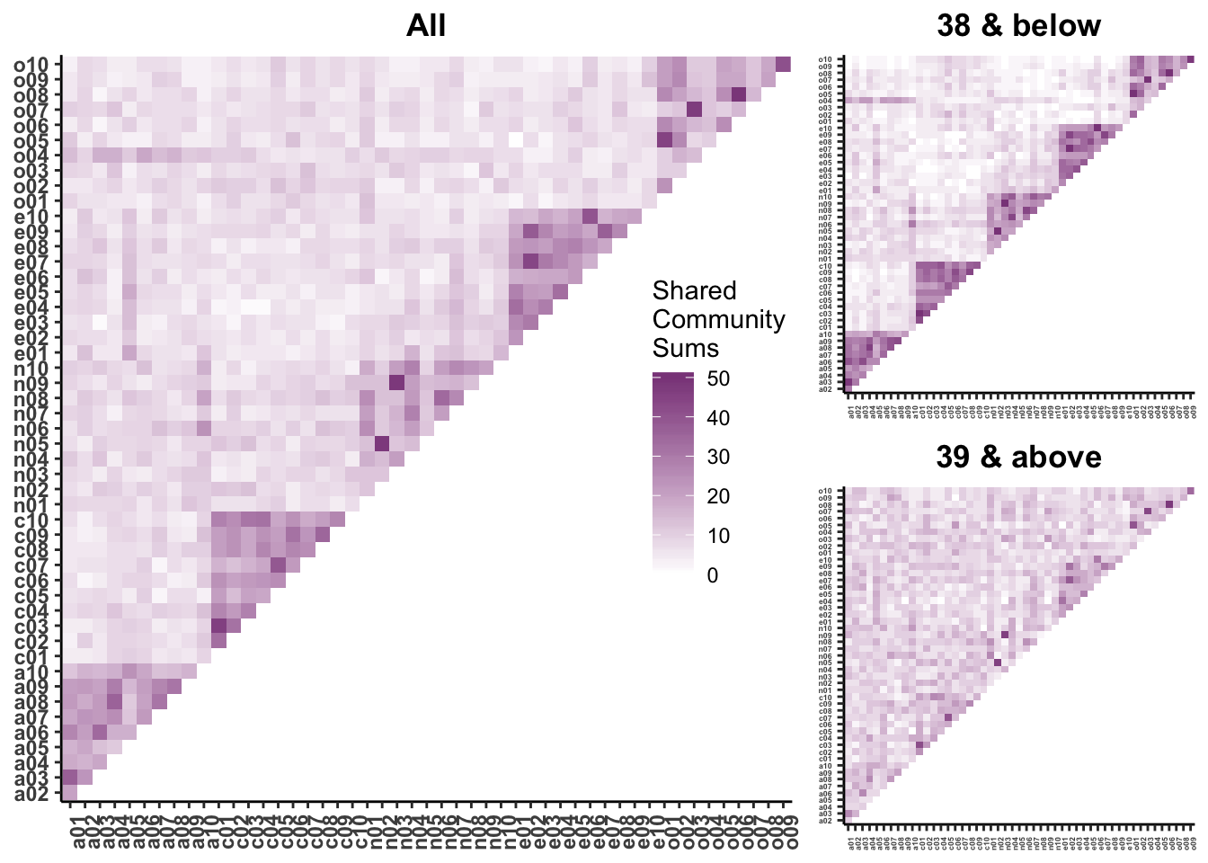
Visualizing correlation matrices
A single correlation can be informative; a correlation matrix is more than the sum of its parts.
Correlation matrices can be used to infer larger patterns of relationships. You may be one of the gifted who can look at a matrix of numbers and see those patterns immediately. Or you can use heat maps to visualize correlation matrices.
Factors that influence \(r\) (and most other test statistics)
Restriction of range (GRE scores and success)
Very skewed distributions (smoking and health)
Non-linear associations
Measurement overlap (modality and content)
Reliability
Reliability
Which would you rather have?
- 1-item final exam versus 30-item?
- assessment via trained clinician vs tarot cards?
- fMRI during minor earthquake vs no earthquake?
All measurement includes error
- Score = true score + measurement error (CTT version)
- Reliability assesses the consistency of measurement; high reliability indicates less error
Reliability
Cannot correlate error (randomness) with something
Because we do not measure our variables perfectly we get lower correlations compared to true correlations
If we want to have a valid measure it better be a reliable measure
Reliability
Think of reliability as a correlation with a measure and itself in a different world, at a different time, or a different but equal version
\[r_{XX}\]
Reliability
Reliability can be expressed as the proportion of true score variance over observed variance
How do you assess theoretical variance i.e., true score variance?
\[r_{XY} = r_{X_{T} Y_{T}} {\sqrt{r_{XX}r_{YY}}}\]
\[r_{XY} = .6 {\sqrt {(.70) (.70)}}\]
Reliability
\[r_{X_{T} Y_{T}} = = {\frac {r_{XY}} {\sqrt{r_{XX}r_{YY}}}}\] \[r_{X_{T} Y_{T}} = = {\frac {.30} {\sqrt{(.70)(.70)}}} = .42\]
Most common ways to assess
Reliability
if you are going to measure something, do it well
applies to ALL IVs and DVs, and all designs
remember this when interpreting research
Types of correlations
Many ways to get at relationship between two variables
Statistically the different types are almost exactly the same
Exist for historical reasons
Types of correlations
- Point Biserial
- continuous and dichotomous
- Phi coefficient
- both dichotomous
- Spearman rank order
- ranked data
- Biserial (assumes dichotomous is continuous)
Some important exceptions to the equivalence rule
- Tetrachoric
- used for 2x2 contingency table
- Polychoric
- ordinal variables
- extension of tetrachoric
Statistics and eugenics
The concept of the correlation is primarily attributed to Sir Frances Galton.
- He was also the founder of the concept of eugenics.
The correlation coefficient was developed by his student, Karl Pearson, and adapted into the ANOVA framework by Sir Ronald Fisher.
- Both were prominent advocates for the eugenics movement.
What do we do with this information?
Never use the correlation or the later techniques developed on it? Of course not.
Acknowledge this history? Certainly.
Understand how the perspectives of Galton, Fisher, Pearson and others shaped our practices? We must! – these are not set in stone, nor are they necessarily the best way to move forward.
- Statistical significance was a way to avoid talking about nuance or degree.
- “Correlation does not imply causation” was a refutation of work demonstrating associations between environment and poverty.
Next time….
Univariate regression