Univariate Regression

Part 1

Last time

• Correlation as inferential test

  • Power

• Fisher’s r to z transformation

• Correlation matrices

• Interpreting effect size

Today

Regression

• What is it? Why is it useful

• Nuts and bolts

  • Equation

  • Ordinary least squares

  • Interpretation

library(psych)
library(tidyverse)
library(broom)
library(here)

Regression

Regression is a general data analytic system, meaning lots of things fall under the umbrella of regression. This system can handle a variety of forms of relations, although all forms have to be specified in a linear way. Usefully, we can incorporate IVs of all nature – continuous, categorical, nominal, ordinal….

The output of regression includes both effect sizes and, if using frequentist or Bayesian software, statistical significance. We can also incorporate multiple influences (IVs) and account for their intercorrelations.

Regression

• Adjustment: Statistically control for known effects

  • If everyone had the same level of SES, would education still predict wealth?

• Prediction: We can develop models based on what’s happened in the past to predict what will happen in the future.

  • Insurance premiums

• Explanation: explaining the influence of one or more variables on some outcome.

  • Does this intervention affect reaction time?

Regression equation

What is a regression equation?

• Functional relationship

  • Ideally like a physical law \(\large (E = MC^2)\)
  • In practice, it’s never as robust as that.
  • Note: this equation may not represent the true causal process!

• How do we uncover the relationship?

How does Y vary with X?

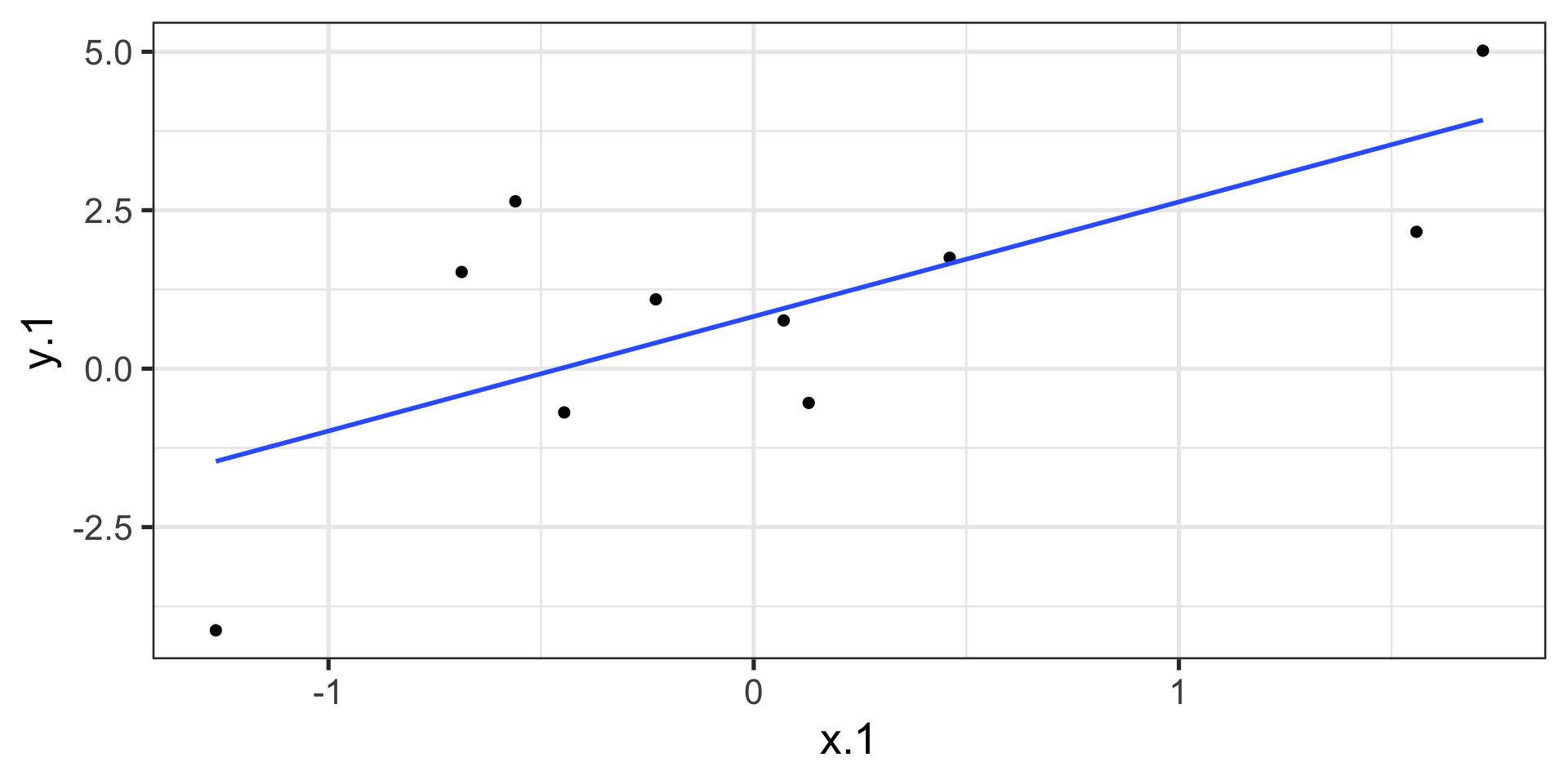
• The regression of Y (DV) on X (IV) corresponds to the line that gives the mean value of Y corresponding to each possible value of X

• \(E(Y|X)\)

• “Our best guess” regardless of whether our model includes categories or continuous predictor variables

Regression Equation

There are two ways to think about our regression equation. They’re similar to each other, but they produce different outputs.

\[Y_i = b_{0} + b_{1}X_i +e_i\]

\[\hat{Y_i} = b_{0} + b_{1}X_i\]

The first is the equation that represents how each observed outcome \((Y_i)\) is calculated. This observed value is the sum of some constant \((b_0)\), the weighted \((b_1)\) observed values of the predictors \((X_i)\) and error \((e_i)\) that cannot be covered by the observed data.

\(\hat{Y}\) signifies the fitted score – no error

The difference between the fitted and observed score is the residual (\(e_i\))

There is a different e value for each observation in the dataset

Regression Equation

\[Y_i = b_{0} + b_{1}X_i + e_i\]

\[\hat{Y_i} = b_{0} + b_{1}X_i\]

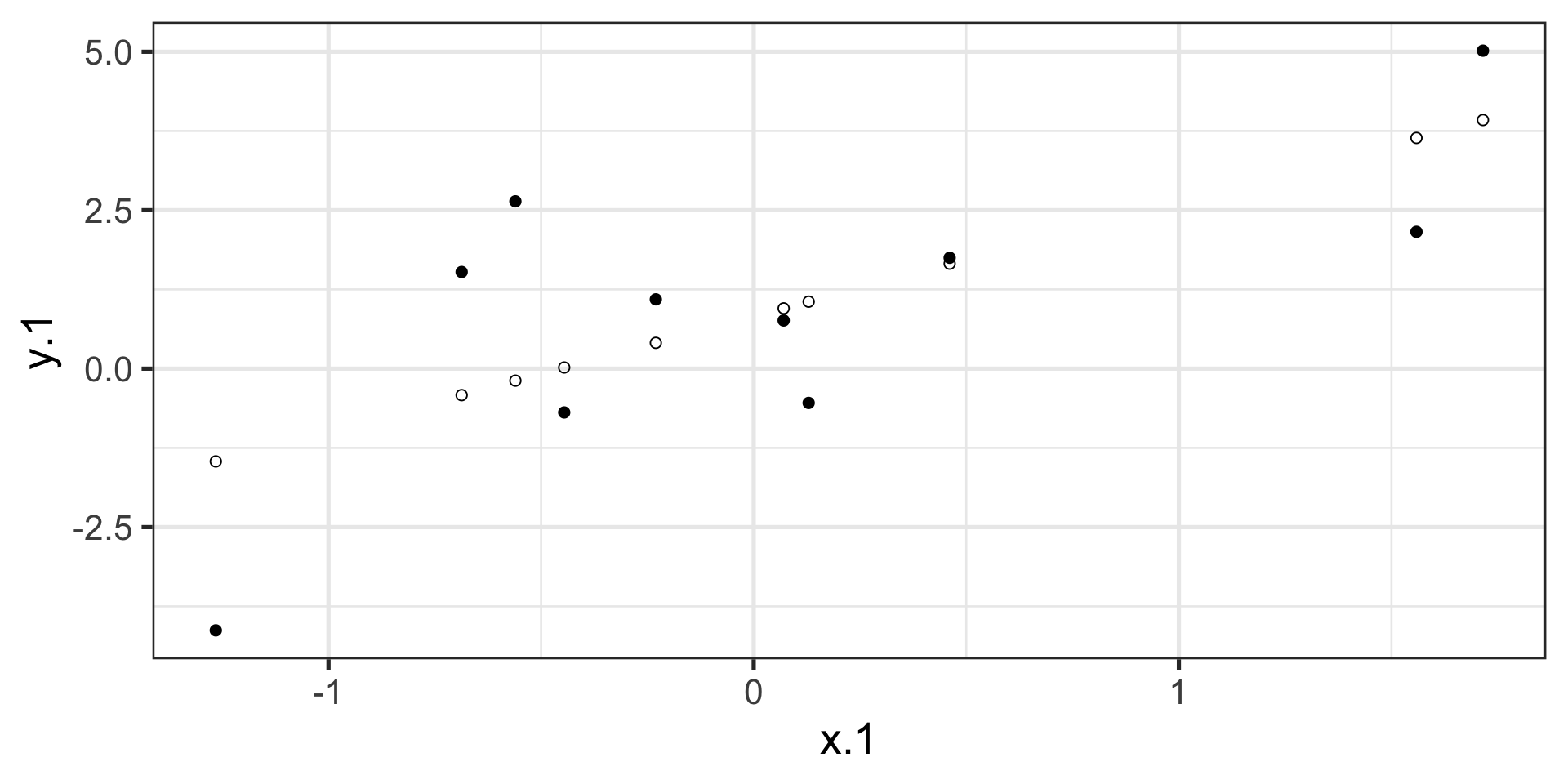
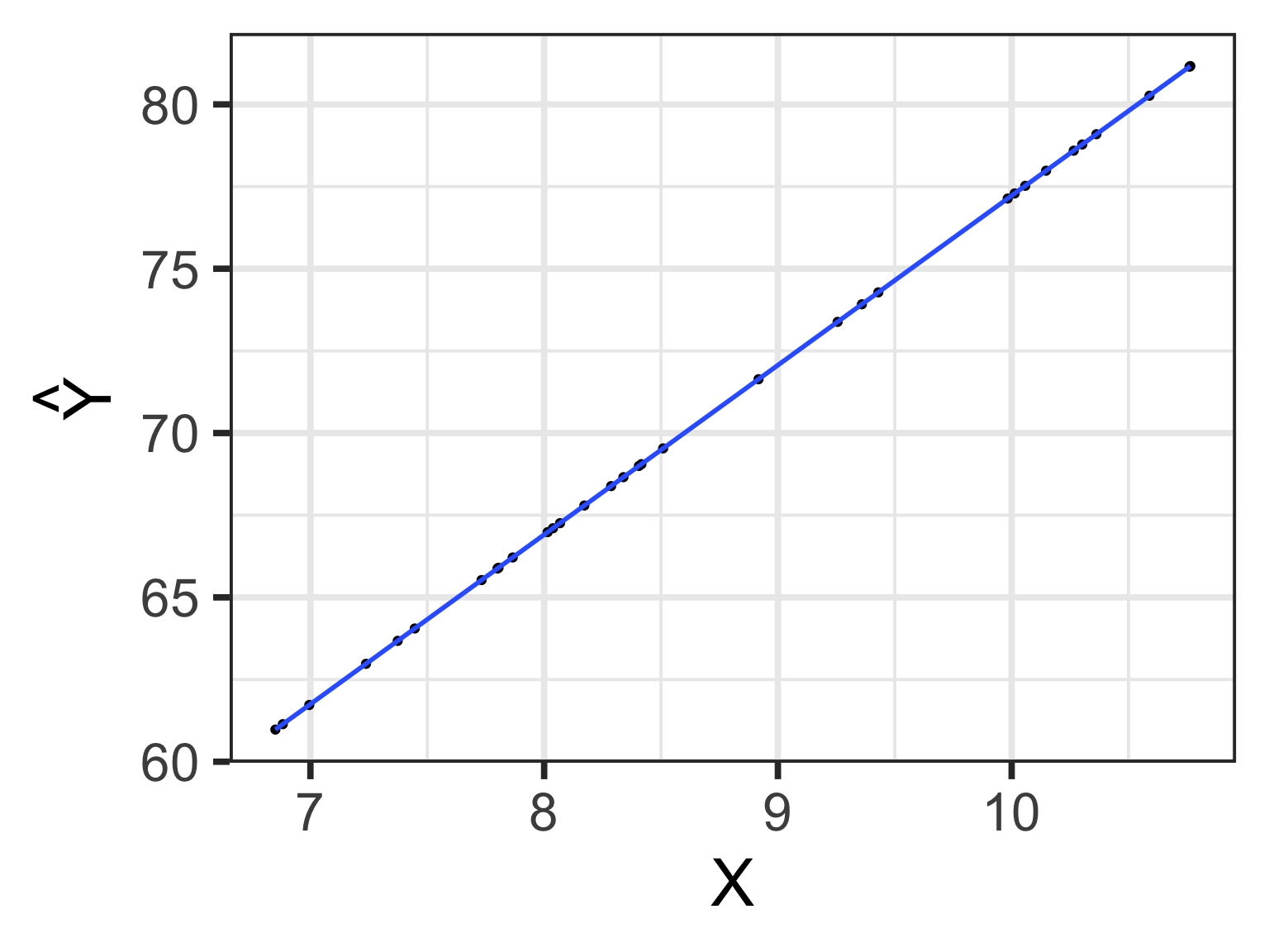
The second is the equation that represents our expected or fitted value of the outcome \((\hat{Y_i})\), sometimes referred to as the “predicted value.” This expected value is the sum of some constant \((b_0)\), the weighted \((b_1)\) observed values of the predictors \((X_i)\).

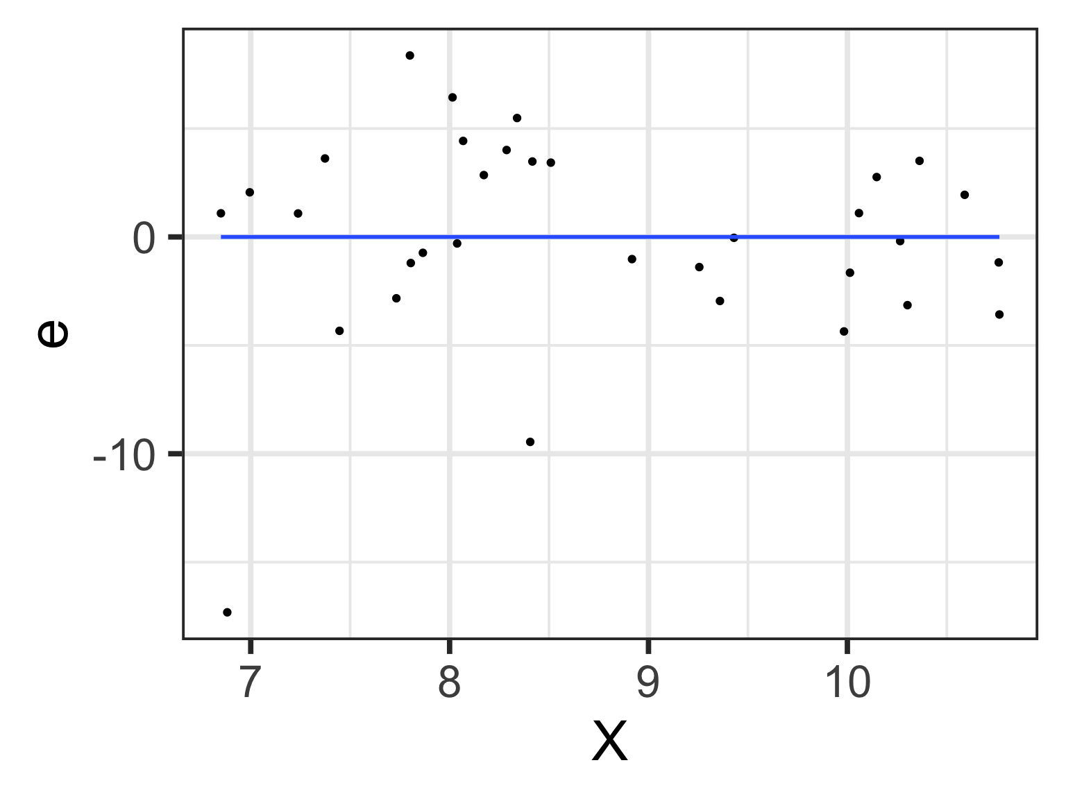
Note that \(Y_i - \hat{Y_i} = e_i\).

\(\hat{Y}\) signifies the fitted score – no error

The difference between the fitted and observed score is the residual (\(e_i\))

There is a different e value for each observation in the dataset

OLS

• How do we find the regression estimates?

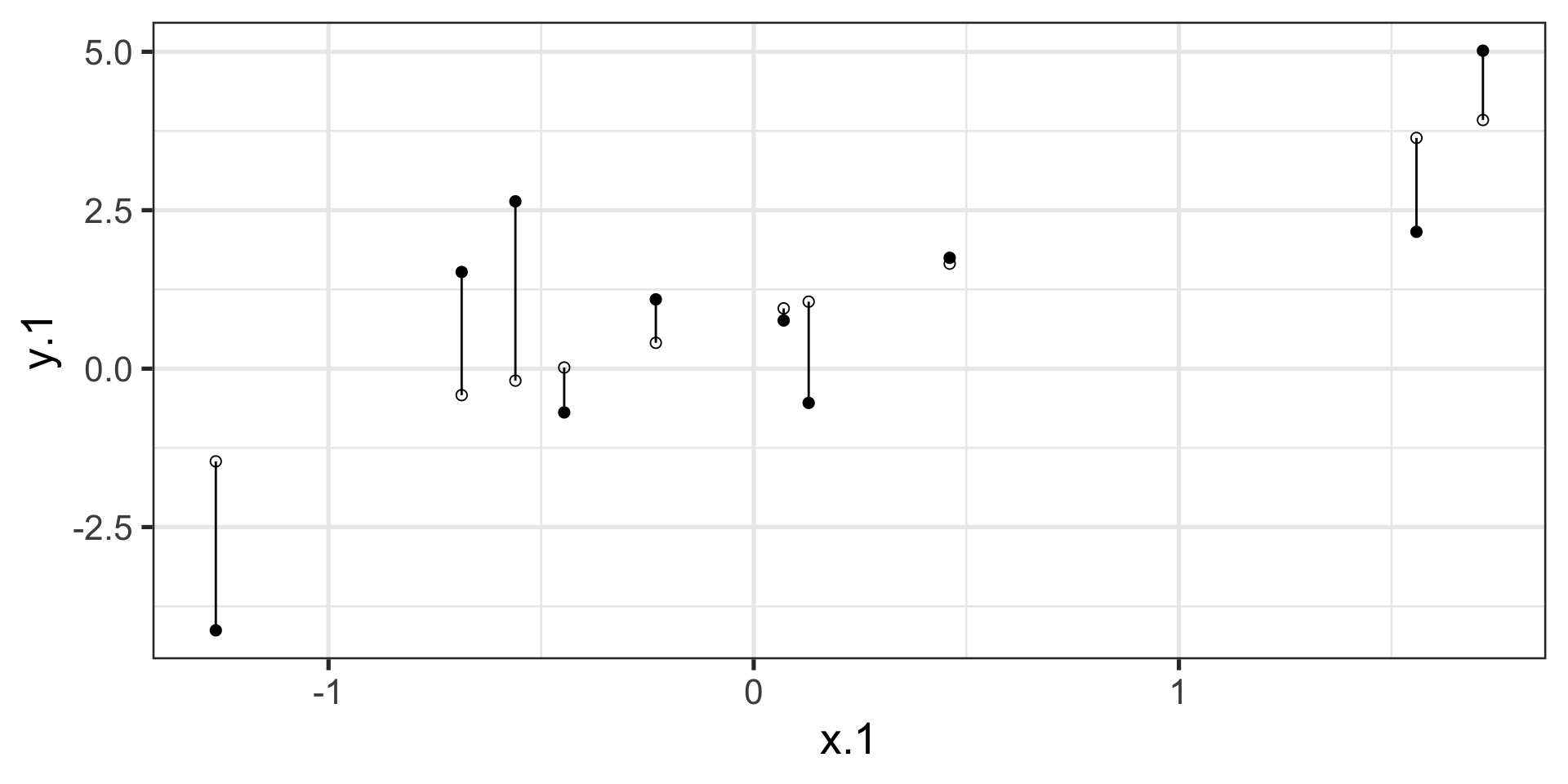
• Ordinary Least Squares (OLS) estimation

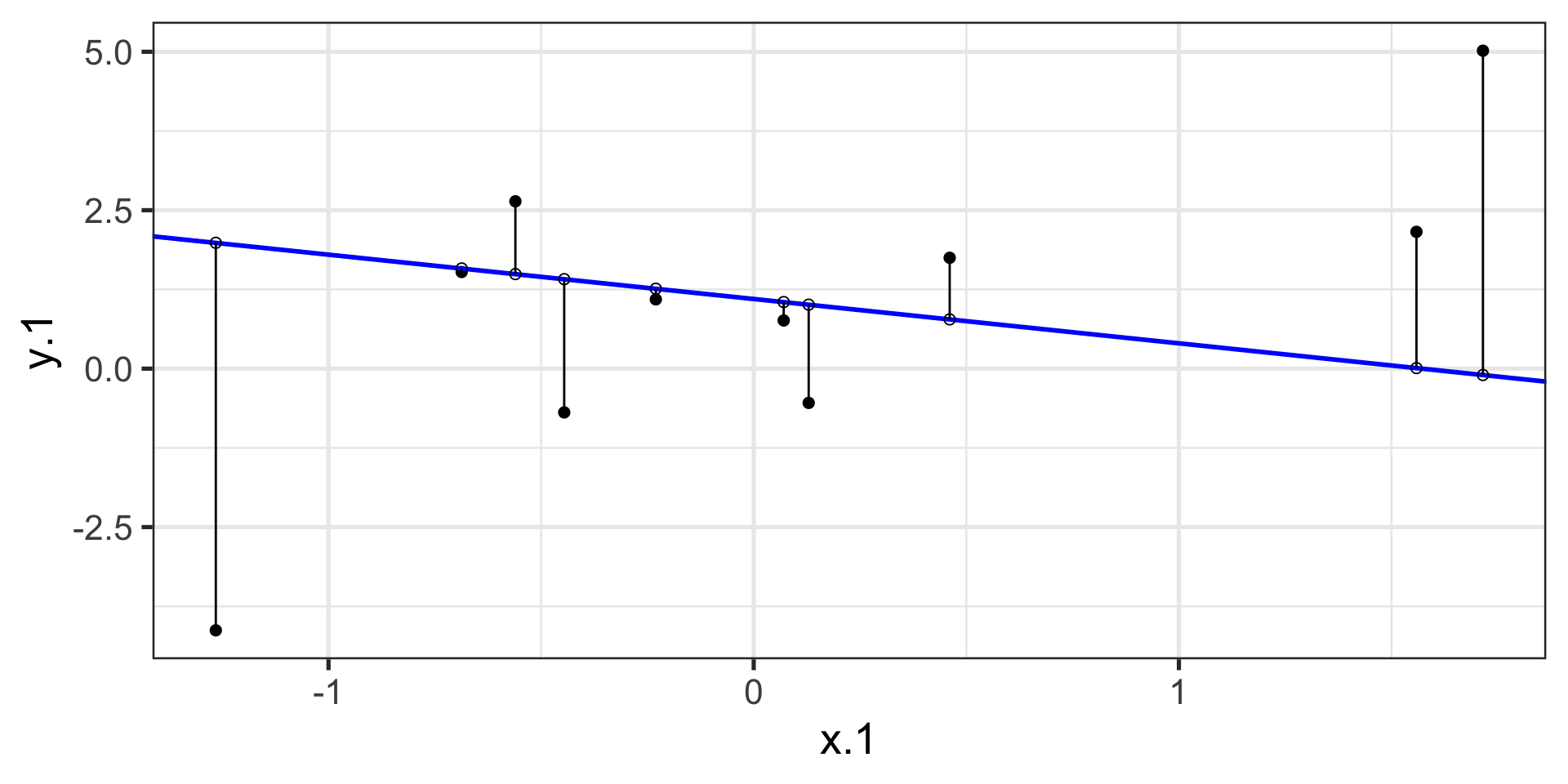
• Minimizes deviations

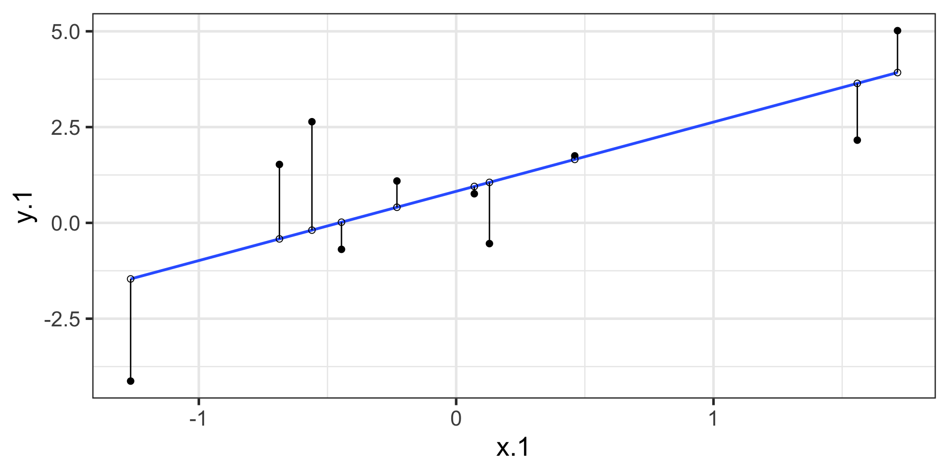
  • \[ min\sum(Y_{i} - \hat{Y} ) ^{2} \]

• Other estimation procedures possible (and necessary in some cases)

Code

ggplot(d1.f , aes(x=x.1, y=y.1)) +
    geom_point(size = 2) +
  geom_smooth(method = lm, se = FALSE) +
  theme_bw(base_size = 20)

Code

ggplot(d1.f , aes(x=x.1, y=y.1)) +
    geom_point(size = 2) +
  geom_point(aes(y = .fitted), shape = 1, size = 2) +
  theme_bw(base_size = 20)

Code

ggplot(d1.f , aes(x=x.1, y=y.1)) +
    geom_point(size = 2) +
  geom_point(aes(y = .fitted), shape = 1, size = 2) +
  geom_segment(aes( xend = x.1, yend = .fitted))+
  theme_bw(base_size = 20)

Code

ggplot(d1.f , aes(x=x.1, y=y.1)) +
    geom_point(size = 2) +
  geom_smooth(method = lm, se = FALSE) +
  geom_point(aes(y = .fitted), shape = 1, size = 2) +
  geom_segment(aes( xend = x.1, yend = .fitted))+
  theme_bw(base_size = 20)

compare to bad fit

\[\Large Y_i = b_{0} + b_{1}X_i +e_i\] \[\Large \hat{Y_i} = b_{0} + b_{1}X_i\] \[\Large Y_i = \hat{Y_i} + e_i\] \[\Large e_i = Y_i - \hat{Y_i}\]

OLS

The line that yields the smallest sum of squared deviations

\[\Sigma(Y_i - \hat{Y_i})^2\] \[= \Sigma(Y_i - (b_0+b_{1}X_i))^2\] \[= \Sigma(e_i)^2\]

In order to find the OLS solution, you could try many different coefficients \((b_0 \text{ and } b_{1})\) until you find the one with the smallest sum squared deviation. Luckily, there are simple calculations that will yield the OLS solution every time.

Regression coefficient, \(b_{1}\)

\[b_{1} = \frac{cov_{XY}}{s_{x}^{2}} = r_{xy} \frac{s_{y}}{s_{x}}\]

What units is the regression coefficient in?

The regression coefficient (slope) equals the estimated change in Y for a 1-unit change in X

\[\Large b_{1} = r_{xy} \frac{s_{y}}{s_{x}}\]

If the standard deviation of both X and Y is equal to 1:

\[\Large b_1 = r_{xy} \frac{s_{y}}{s_{x}} = r_{xy} \frac{1}{1} = r_{xy} = \beta_{yx} = b_{yx}^*\]

Standardized regression equation

\[\Large Z_{y_i} = b_{yx}^*Z_{x_i}+e_i\]

\[\Large b_{yx}^* = b_{yx}\frac{s_x}{s_y} = r_{xy}\]

According to this regression equation, when \(X = 0, Y = 0\). Our interpretation of the coefficient is that a one-standard deviation increase in X is associated with a \(b_{yx}^*\) standard deviation increase in Y. Our regression coefficient is equivalent to the correlation coefficient when we have only one predictor in our model.

Estimating the intercept, \(b_0\)

• intercept serves to adjust for differences in means between X and Y

\[\hat{Y_i} = \bar{Y} + r_{xy} \frac{s_{y}}{s_{x}}(X_i-\bar{X})\]

• if standardized, intercept drops out

• otherwise, intercept is where regression line crosses the y-axis at X = 0

• Also, notice that when \(X = \bar{X}\) the regression line goes through \(\bar{Y}\)

\[b_0 = \bar{Y} - b_1\bar{X}\]

The intercept adjusts the location of the regression line to ensure that it runs through the point \(\large (\bar{X}, \bar{Y}).\) We can calculate this value using the equation:

\[\Large b_0 = \bar{Y} - b_1\bar{X}\]

Example

library(gapminder)
gapminder = gapminder %>% filter(year == 2007 & continent == "Asia") %>% 
  mutate(log_gdp = log(gdpPercap))
describe(gapminder[,c("log_gdp", "lifeExp")], fast = T)

        vars  n  mean   sd   min   max range   se
log_gdp    1 33  8.74 1.24  6.85 10.76  3.91 0.22
lifeExp    2 33 70.73 7.96 43.83 82.60 38.77 1.39

cor(gapminder$log_gdp, gapminder$lifeExp)

[1] 0.8003474

If we regress lifeExp onto log_gdp:

r = cor(gapminder$log_gdp, gapminder$lifeExp)
m_log_gdp = mean(gapminder$log_gdp)
m_lifeExp = mean(gapminder$lifeExp)
s_log_gdp = sd(gapminder$log_gdp)
s_lifeExp = sd(gapminder$lifeExp)

b1 = r*(s_lifeExp/s_log_gdp)

[1] 5.157259

b0 = m_lifeExp - b1*m_log_gdp

[1] 25.65011

How will this change if we regress GDP onto life expectancy?

(b1 = r*(s_lifeExp/s_log_gdp))

[1] 5.157259

(b0 = m_lifeExp - b1*m_log_gdp)

[1] 25.65011

(b1 = r*(s_log_gdp/s_lifeExp))

[1] 0.1242047

(b0 = m_log_gdp - b1*m_lifeExp)

[1] -0.04405086

In R

fit.1 <- lm(lifeExp ~ log_gdp, data = gapminder)
summary(fit.1)

Call:
lm(formula = lifeExp ~ log_gdp, data = gapminder)

Residuals:
    Min      1Q  Median      3Q     Max 
-17.314  -1.650  -0.040   3.428   8.370 

Coefficients:
            Estimate Std. Error t value     Pr(>|t|)    
(Intercept)  25.6501     6.1234   4.189     0.000216 ***
log_gdp       5.1573     0.6939   7.433 0.0000000226 ***
---
Signif. codes:  0 '***' 0.001 '**' 0.01 '*' 0.05 '.' 0.1 ' ' 1

Residual standard error: 4.851 on 31 degrees of freedom
Multiple R-squared:  0.6406,    Adjusted R-squared:  0.629 
F-statistic: 55.24 on 1 and 31 DF,  p-value: 0.00000002263

Things to discuss

• Coefficient estimates
• Statistical tests (covered in more detail soon)

Data, fitted, and residuals

library(broom)
model_info = augment(fit.1)
head(model_info)

# A tibble: 6 × 8
  lifeExp log_gdp .fitted .resid   .hat .sigma .cooksd .std.resid
    <dbl>   <dbl>   <dbl>  <dbl>  <dbl>  <dbl>   <dbl>      <dbl>
1    43.8    6.88    61.1 -17.3  0.101    3.63 0.796       -3.76 
2    75.6   10.3     78.8  -3.15 0.0802   4.89 0.0199      -0.676
3    64.1    7.24    63.0   1.08 0.0765   4.93 0.00224      0.233
4    59.7    7.45    64.1  -4.33 0.0646   4.86 0.0294      -0.923
5    73.0    8.51    69.5   3.43 0.0314   4.89 0.00836      0.718
6    82.2   10.6     80.3   1.94 0.100    4.92 0.00994      0.422

describe(model_info, fast = T)

           vars  n  mean   sd    min   max range   se
lifeExp       1 33 70.73 7.96  43.83 82.60 38.77 1.39
log_gdp       2 33  8.74 1.24   6.85 10.76  3.91 0.22
.fitted       3 33 70.73 6.37  60.98 81.16 20.19 1.11
.resid        4 33  0.00 4.77 -17.31  8.37 25.68 0.83
.hat          5 33  0.06 0.03   0.03  0.11  0.08 0.00
.sigma        6 33  4.84 0.23   3.63  4.93  1.30 0.04
.cooksd       7 33  0.04 0.14   0.00  0.80  0.80 0.02
.std.resid    8 33  0.00 1.02  -3.76  1.77  5.53 0.18

Point out the average of the residuals is 0, just like average deviation from the mean is 0.

The relationship between \(X_i\) and \(\hat{Y_i}\)

Code

model_info %>% ggplot(aes(x = log_gdp, y = .fitted)) +
  geom_point() + geom_smooth(se = F, method = "lm") +
  scale_x_continuous("X") + scale_y_continuous(expression(hat(Y))) + theme_bw(base_size = 30)

The relationship between \(X_i\) and \(e_i\)

Code

model_info %>% ggplot(aes(x = log_gdp, y = .resid)) +
  geom_point() + geom_smooth(se = F, method = "lm") + 
  scale_x_continuous("X") + scale_y_continuous("e") + theme_bw(base_size = 30)

The relationship between \(Y_i\) and \(\hat{Y_i}\)

Code

model_info %>% ggplot(aes(x = lifeExp, y = .fitted)) +
  geom_point() + geom_smooth(se = F, method = "lm") + 
  scale_x_continuous("Y") + scale_y_continuous(expression(hat(Y))) + theme_bw(base_size = 30)

The relationship between \(Y_i\) and \(e_i\)

Code

model_info %>% ggplot(aes(x = lifeExp, y = .resid)) +
  geom_point() + geom_smooth(se = F, method = "lm") + 
  scale_x_continuous("Y") + scale_y_continuous("e") + theme_bw(base_size = 25)

The relationship between \(\hat{Y_i}\) and \(e_i\)

Code

model_info %>% ggplot(aes(x = .fitted, y = .resid)) +
  geom_point() + geom_smooth(se = F, method = "lm") + 
  scale_y_continuous("e") + scale_x_continuous(expression(hat(Y))) + theme_bw(base_size = 30)

Regression to the mean

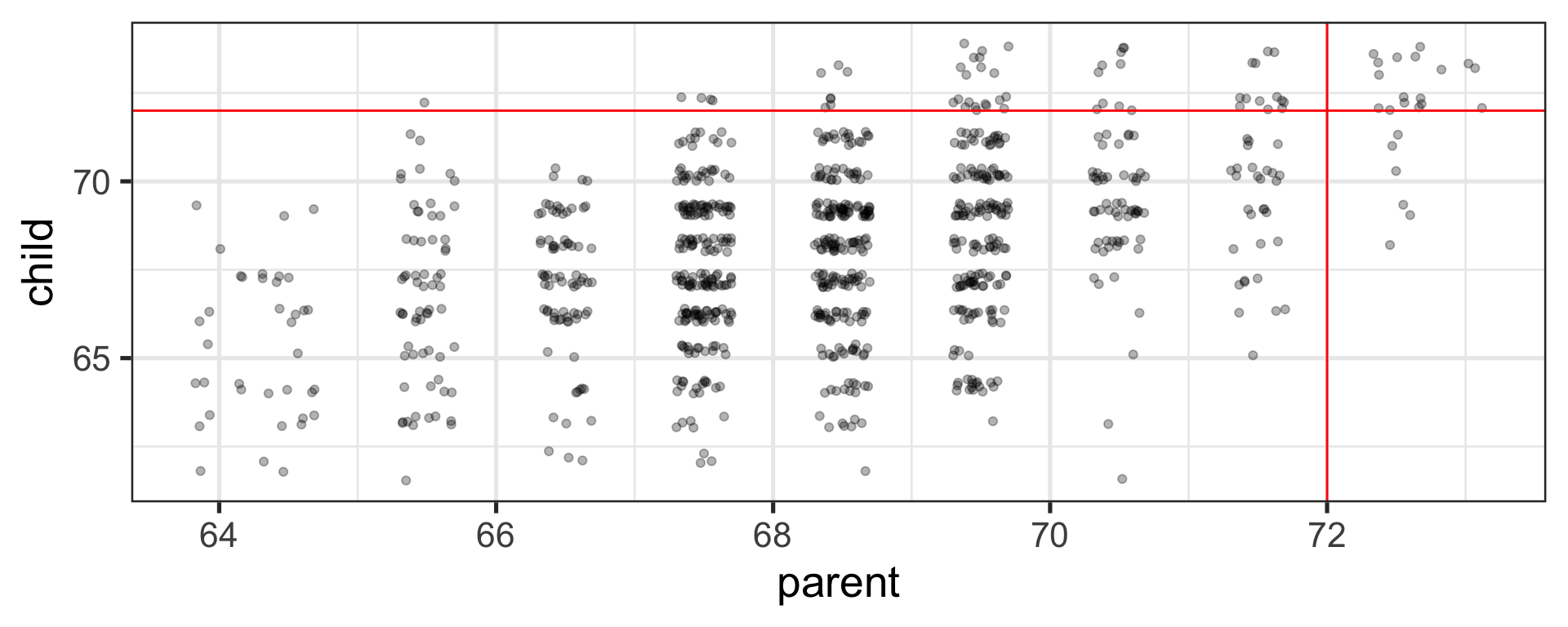
An observation about heights was part of the motivation to develop the regression equation: If you selected a parent who was exceptionally tall (or short), their child was almost always not as tall (or as short).

Code

library(psychTools)
library(tidyverse)
heights = psychTools::galton
mod = lm(child~parent, data = heights)
point = 902
heights = broom::augment(mod)


heights %>%
  ggplot(aes(x = parent, y = child)) +
  geom_jitter(alpha = .3) +
  geom_hline(aes(yintercept = 72), color = "red") +
  geom_vline(aes(xintercept = 72), color = "red") +
  theme_bw(base_size = 20)

Regression to the mean

This phenomenon is known as regression to the mean. This describes the phenomenon in which an random variable produces an extreme score on a first measurement, but a lower score on a second measurement.

We can see this in the standardized regression equation:

\[\hat{Y_i} = r_{xy}(X_i) + e_i\] In that the slope coefficient can never be greater than 1.

Regression to the mean

This can be a threat to internal validity if interventions are applied based on first measurement scores.

]

Next time…

Statistical inferences with regression