Univariate Regression

Part 3

Last week

Unstandardized regression equation

\[Y = b_0 + b_1X + e\]

• Intercept and slope are interpreted in the units of Y.
  • Useful if the units of Y are meaningful.
• Built from covariances and variances

\[b_1 = \frac{cov_{XY}}{s^2_X}\]

Standardized regression equation

\[Z_Y = b^*_1Z_X + e\]

• Slope are interpreted in standardized units.
  • Useful for comparison
• Built from correlations

\[b^*_1 = r_{xy}\]

options(scipen = 999)
knitr::opts_chunk$set(message = FALSE) # suppress messages
library(tidyverse)
library(broom)
library(gganimate)
library(ungeviz) #download from github

Last week – Inferential tests

Omnibus test

• Does the model fit the data?

• F-test (ratio of variances)

  • How many magnitudes larger is variability attributed to the model compared to left-over variability?

• Effect size: Model fit can be measured in terms of \(\large R^2\) or \(\large s_{Y|X}\)

Terminology

• \(R^2\)

  • coefficient of determination
  • squared correlation between \(Y\) and \(\hat{Y}\)
  • proportion of variance in Y accounted for by the model

• \(s_{Y|X}\)

  • standard error of the estimate and the square root of the mean square error (MSE)
  • measure of discrepancy between model and data
  • estimate of population SD of \(e\)
  • MSE: variance around fitted regression line

Example

Overclaiming occurs when people claim that they know something that is impossible to know; are experts susceptible to overclaiming?

Participants¹ completed a measure of self-perceived knowledge, in which they indicate their level of knowledge in the area of personal finance. Next participants indicated how much they knew about 15 terms related to personal finance (e.g., home equity). Included in the 15 items were three terms that do not actually exist (e.g., annualized credit). Thus, overclaiming occurred when participants said that they were knowledgeable about the non-existent terms.

1. Atir, S., Rosenzweig, E., & Dunning, D. (2015). When knowledge knows no bounds: Self-perceived expertise predicts claims of impossible knowledge. Psychological Science, 26, 1295-1303.

library(here)
expertise = read.csv(here("data/expertise.csv"))
psych::describe(expertise)

                         vars   n   mean    sd median trimmed   mad   min
id                          1 202 101.50 58.46 101.50  101.50 74.87  1.00
order_of_tasks              2 202   1.50  0.50   1.50    1.50  0.74  1.00
self_perceived_knowledge    3 202   4.43  1.17   4.50    4.45  0.74  1.00
overclaiming_proportion     4 202   0.31  0.23   0.28    0.29  0.25  0.00
accuracy                    5 202   0.30  0.21   0.28    0.29  0.21 -0.19
FINRA_score                 6 202   3.70  1.19   4.00    3.85  1.48  0.00
                            max  range  skew kurtosis   se
id                       202.00 201.00  0.00    -1.22 4.11
order_of_tasks             2.00   1.00  0.00    -2.01 0.04
self_perceived_knowledge   7.00   6.00 -0.20     0.15 0.08
overclaiming_proportion    1.00   1.00  0.64    -0.31 0.02
accuracy                   0.93   1.12  0.28    -0.07 0.01
FINRA_score                5.00   5.00 -1.01     0.57 0.08

cor(expertise[,c("self_perceived_knowledge", "overclaiming_proportion")])

                         self_perceived_knowledge overclaiming_proportion
self_perceived_knowledge                1.0000000               0.4811502
overclaiming_proportion                 0.4811502               1.0000000

fit.1 = lm(overclaiming_proportion ~ self_perceived_knowledge, 
           data = expertise)
anova(fit.1)

Analysis of Variance Table

Response: overclaiming_proportion
                          Df Sum Sq Mean Sq F value             Pr(>F)    
self_perceived_knowledge   1 2.5095 2.50948  60.249 0.0000000000004225 ***
Residuals                200 8.3303 0.04165                               
---
Signif. codes:  0 '***' 0.001 '**' 0.01 '*' 0.05 '.' 0.1 ' ' 1

summary(fit.1)

Call:
lm(formula = overclaiming_proportion ~ self_perceived_knowledge, 
    data = expertise)

Residuals:
     Min       1Q   Median       3Q      Max 
-0.50551 -0.15610  0.00662  0.12167  0.54215 

Coefficients:
                         Estimate Std. Error t value          Pr(>|t|)    
(Intercept)              -0.11406    0.05624  -2.028            0.0439 *  
self_perceived_knowledge  0.09532    0.01228   7.762 0.000000000000422 ***
---
Signif. codes:  0 '***' 0.001 '**' 0.01 '*' 0.05 '.' 0.1 ' ' 1

Residual standard error: 0.2041 on 200 degrees of freedom
Multiple R-squared:  0.2315,    Adjusted R-squared:  0.2277 
F-statistic: 60.25 on 1 and 200 DF,  p-value: 0.0000000000004225

library(sjPlot)
set_theme(base = theme_bw())

plot_model(fit.1, 
           type = "pred", 
           show.data = T) 

plot_model(fit.1, 
           type = "pred", show.data = T, 
           jitter = T) 

Point out here: * Can be hard to visualize data when you have a Likert scale or other measure with a relatively small number of possible answers. * BUT jitter can produce impossible data points and possibly hide floor or ceiling effects.

regression coefficient

\[\Large H_{0}: \beta_{1}= 0\] \[\Large H_{1}: \beta_{1} \neq 0\]

What does the regression coefficient test?

• Does X provide any predictive information?

• Does X provide any explanatory power regarding the variability of Y?

• Is the the average value different from the best guess

  • (i.e., is \(\bar{Y}\) equal to \(\hat{Y}\) ?)

• Is the regression line not flat?

• Are X and Y correlated?

Regression coefficient

\[\Large se_{b} = \frac{s_{Y}}{s_{X}}{\sqrt{\frac {1-r_{xy}^2}{n-2}}}\] \[\Large t(n-2) = \frac{b_{1}}{se_{b}}\]

summary(fit.1)

Call:
lm(formula = overclaiming_proportion ~ self_perceived_knowledge, 
    data = expertise)

Residuals:
     Min       1Q   Median       3Q      Max 
-0.50551 -0.15610  0.00662  0.12167  0.54215 

Coefficients:
                         Estimate Std. Error t value          Pr(>|t|)    
(Intercept)              -0.11406    0.05624  -2.028            0.0439 *  
self_perceived_knowledge  0.09532    0.01228   7.762 0.000000000000422 ***
---
Signif. codes:  0 '***' 0.001 '**' 0.01 '*' 0.05 '.' 0.1 ' ' 1

Residual standard error: 0.2041 on 200 degrees of freedom
Multiple R-squared:  0.2315,    Adjusted R-squared:  0.2277 
F-statistic: 60.25 on 1 and 200 DF,  p-value: 0.0000000000004225

\(se_b\)

• standard error for the slope coefficient

• represent our uncertainty (noise) in our estimate of the regression coefficient

• different from (but proportional to) the standard error of the estimate

• we can take our estimate \((b)\) and put confidence regions around it to get an estimate of what could be “possible” if we ran the study again

Intercept

• more complex standard error calculation

• the calculation depends on how far the X value (here zero) is away from the mean of X

  • farther from the mean, less information, thus more uncertainty

• we’ll come back to this calculation shortly

summary(fit.1)

Call:
lm(formula = overclaiming_proportion ~ self_perceived_knowledge, 
    data = expertise)

Residuals:
     Min       1Q   Median       3Q      Max 
-0.50551 -0.15610  0.00662  0.12167  0.54215 

Coefficients:
                         Estimate Std. Error t value          Pr(>|t|)    
(Intercept)              -0.11406    0.05624  -2.028            0.0439 *  
self_perceived_knowledge  0.09532    0.01228   7.762 0.000000000000422 ***
---
Signif. codes:  0 '***' 0.001 '**' 0.01 '*' 0.05 '.' 0.1 ' ' 1

Residual standard error: 0.2041 on 200 degrees of freedom
Multiple R-squared:  0.2315,    Adjusted R-squared:  0.2277 
F-statistic: 60.25 on 1 and 200 DF,  p-value: 0.0000000000004225

Confidence interval for coefficients

• same equation as we’ve been working with:

\[CI_b = b \pm CV(se_b)\]

• How do we estimate the critical value?

coef(summary(fit.1))

                            Estimate Std. Error   t value              Pr(>|t|)
(Intercept)              -0.11405571 0.05624236 -2.027932 0.0438935615758865028
self_perceived_knowledge  0.09531747 0.01227997  7.762029 0.0000000000004224832

confint(fit.1)

                               2.5 %       97.5 %
(Intercept)              -0.22495982 -0.003151603
self_perceived_knowledge  0.07110265  0.119532290

\(b_1 \pm CV(se_b) = 0.095 \pm 1.972(0.012)\) \(b_1 \pm CV(se_b) = 0.095 \pm 0.024\)

\(se_{\hat{Y_i}}\)

In addition to estimating precision around the our coefficients, we can also estimate our precision around our predicted values, \(\hat{Y_i}\). Why might this be a useful exercise?

The formula to estimate the standard error of any particular \(\hat{Y_i}\) is

\[se_{\hat{Y}_i} = s_{Y|X}*\sqrt{\frac {1}{n}+\frac{(X_i-\bar{X})^2}{(n-1)s_{X}^2}}\]

library(broom)
model_info = augment(fit.1, se_fit = T)
psych::describe(model_info, fast=T)

                         vars   n mean   sd   min  max range   se
overclaiming_proportion     1 202 0.31 0.23  0.00 1.00  1.00 0.02
self_perceived_knowledge    2 202 4.43 1.17  1.00 7.00  6.00 0.08
.fitted                     3 202 0.31 0.11 -0.02 0.55  0.57 0.01
.se.fit                     4 202 0.02 0.01  0.01 0.04  0.03 0.00
.resid                      5 202 0.00 0.20 -0.51 0.54  1.05 0.01
.hat                        6 202 0.01 0.01  0.00 0.05  0.04 0.00
.sigma                      7 202 0.20 0.00  0.20 0.20  0.00 0.00
.cooksd                     8 202 0.01 0.01  0.00 0.09  0.09 0.00
.std.resid                  9 202 0.00 1.00 -2.50 2.68  5.18 0.07

head(model_info[,c(".fitted", ".se.fit")])

# A tibble: 6 × 2
  .fitted .se.fit
    <dbl>   <dbl>
1   0.410  0.0195
2   0.315  0.0144
3   0.220  0.0183
4   0.458  0.0241
5   0.124  0.0277
6   0.553  0.0347

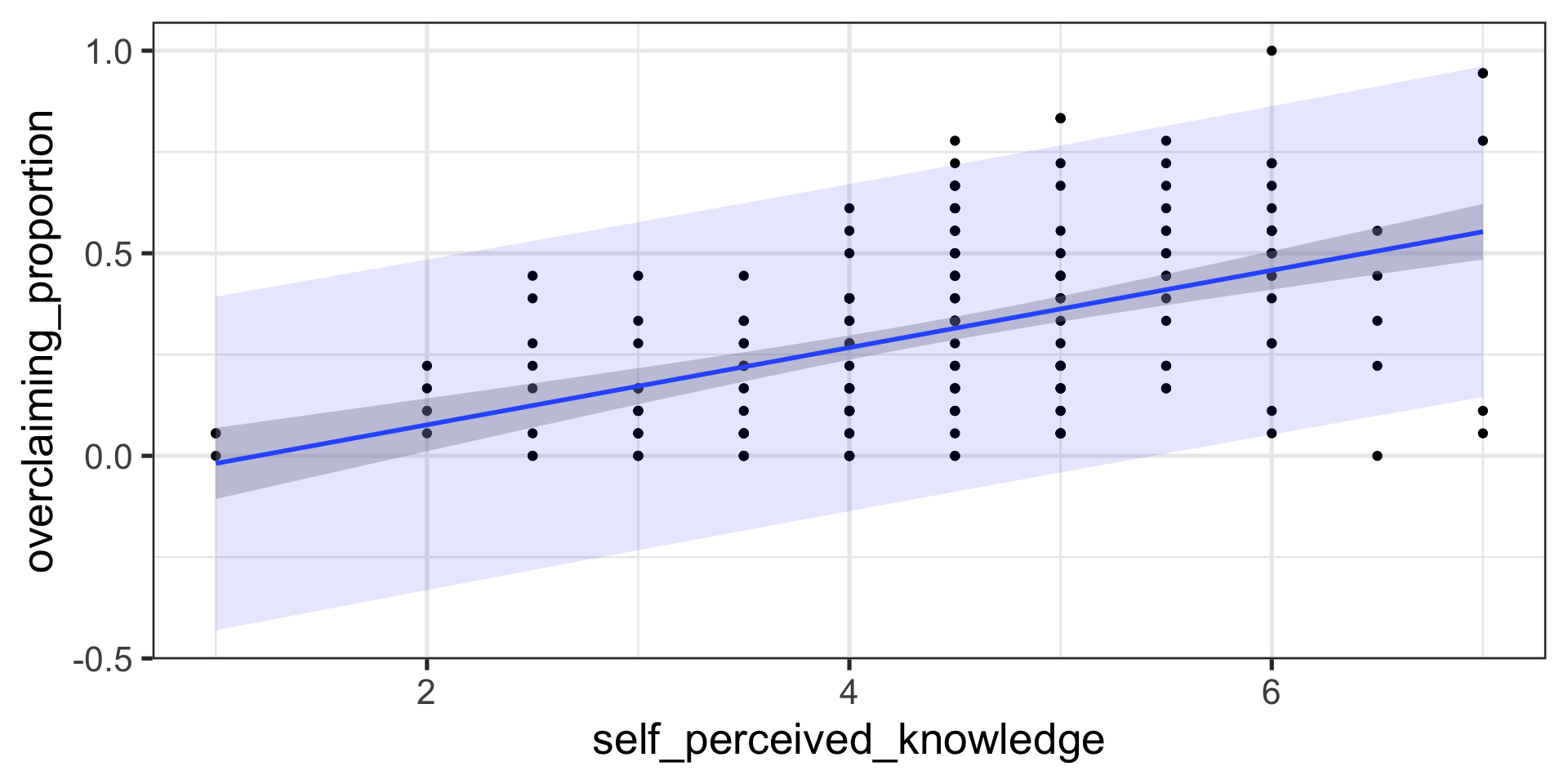
We can string these together in a figure and create confidence bands.

Code

cv = qt(.975, df = nrow(model_info)-2)
model_info %>% 
  ggplot(aes(x = self_perceived_knowledge)) +
  geom_point(aes(y = .fitted)) +
  geom_errorbar(aes(ymin = .fitted-(cv*.se.fit), 
                    ymax = .fitted+(cv*.se.fit)  ))

Code

cv = qt(.975, df = nrow(model_info)-2)
model_info %>% 
  ggplot(aes(x = self_perceived_knowledge)) +
  geom_point(aes(y = .fitted)) +
  geom_errorbar(aes(ymin = .fitted-(cv*.se.fit), 
                    ymax = .fitted+(cv*.se.fit)  )) +
  geom_smooth(aes(y = overclaiming_proportion), method = "lm")

Code

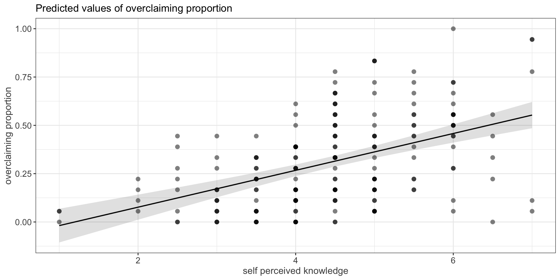
expertise %>%
  ggplot(aes(x = self_perceived_knowledge, y = overclaiming_proportion)) + 
  geom_jitter(size = .5, color = "darkgrey") + 
  geom_smooth(method = "lm") +
  scale_x_continuous("Self-perceived knowledge") +
  scale_y_continuous("Proportion of overclaiming") +
  ggtitle("Using geom_smooth(se = TRUE)")+
  theme_bw()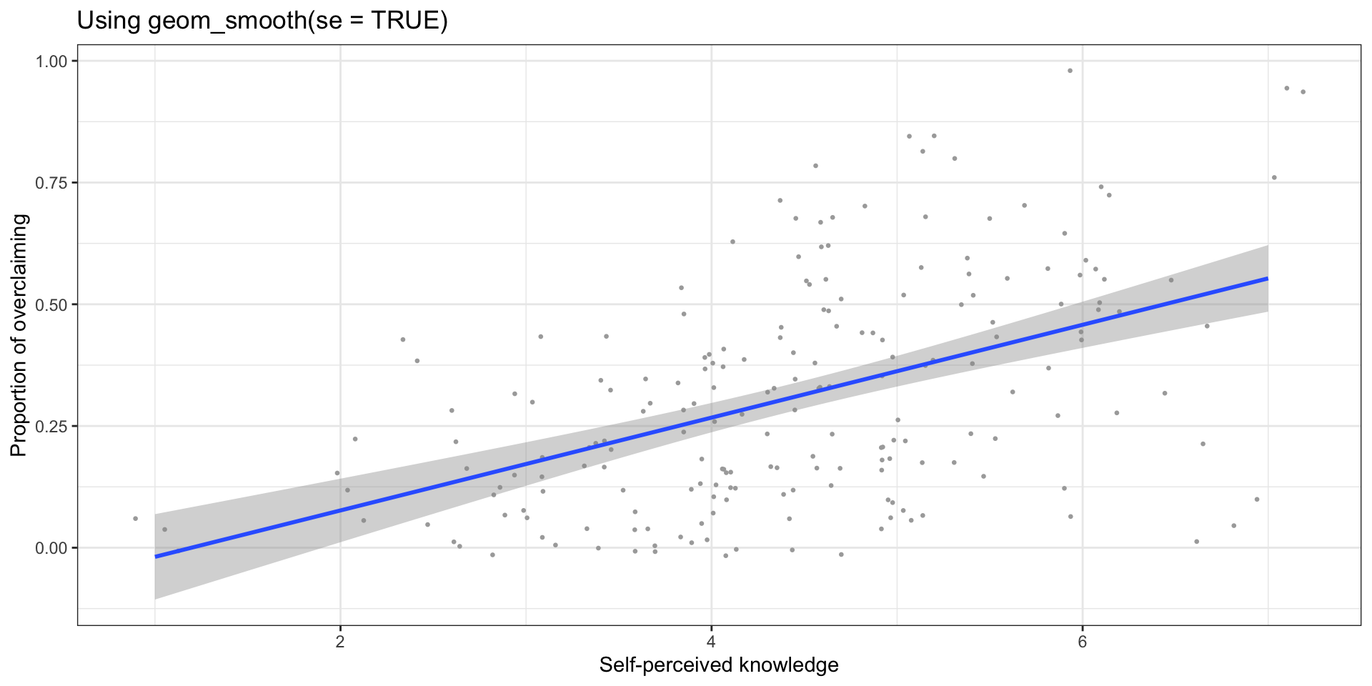

Let’s return to the idea of the uncertainty around our slope and intercept estimates.

confint(fit.1)

                               2.5 %       97.5 %
(Intercept)              -0.22495982 -0.003151603
self_perceived_knowledge  0.07110265  0.119532290

We accept that these ranges represent our guess for where the true values of these parameters could be. So while we estimated a single slope and single intercept, reasonably, there is a set of slopes and intercepts that we would consider reasonable.

What if we took the extremes from these distributions?

\(\hat{Y}_i = -0.22 + 0.12X_i\)

\(\hat{Y}_i = 0 + 0.07X_i\)

Code

expertise %>%
  ggplot(aes(x = self_perceived_knowledge, y = overclaiming_proportion)) + 
  geom_jitter(size = .5, color = "darkgrey") + 
  geom_smooth(method = "lm") +
  geom_abline(aes(intercept = ci[1,1], slope = ci[2,2])) +
  geom_abline(aes(intercept = ci[1,2], slope = ci[2,1])) +
  scale_x_continuous("Self-perceived knowledge") +
  scale_y_continuous("Proportion of overclaiming") +
  theme_bw()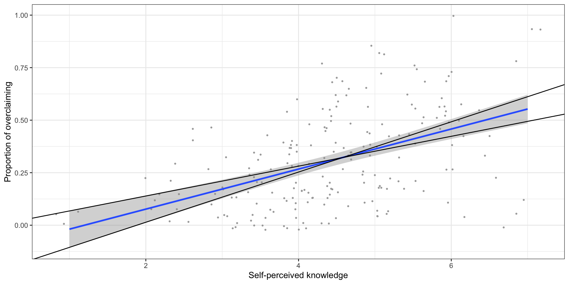

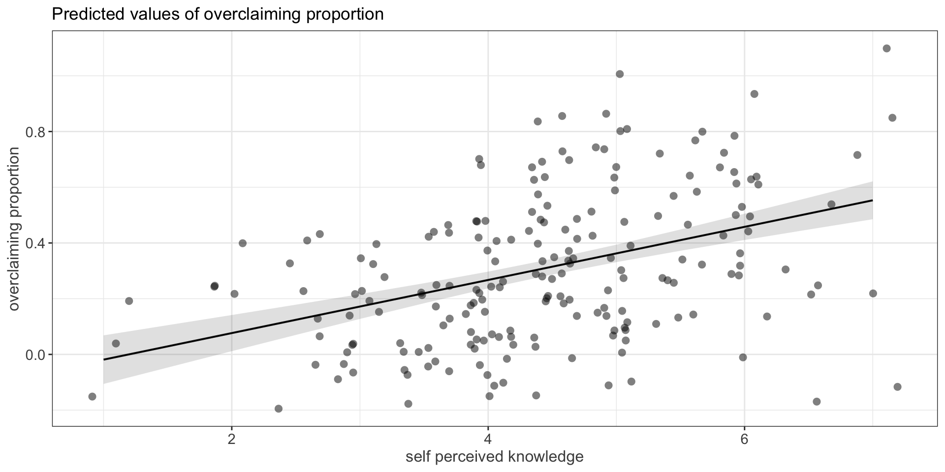
Code

set.seed(012220)

boots <- bootstrapper(100)

p <- expertise %>%
  ggplot(aes(x = self_perceived_knowledge, y = overclaiming_proportion)) +
  geom_smooth(method = "lm", color = NA) +
  geom_jitter(alpha = 0.3) +
  geom_smooth(data = boots, method = "lm", fullrange = TRUE, se = FALSE) +
  theme_minimal() +
  transition_states(.draw, 1, 1) +
  enter_fade() +
  exit_fade() +
  ease_aes()

animate(p, fps = 3)

Confidence Bands for regression line

Code

set.seed(123)

px.1 <- rnorm(1000, 0, 1)
pe.1 <- rnorm(1000, 0, 1)
py.1 <- .5 + .55 * px.1 + pe.1
pd.1 <- data.frame(px.1,py.1)

px.2 <- rnorm(100, 0, 1)
pe.2 <- rnorm(100, 0, 1)
py.2 <- .5 + .55 * px.2 + pe.2
pd.2 <- data.frame(px.2,py.2)


p1 <- ggplot(pd.1, aes(x = px.1,y =  py.1)) +
    geom_point(alpha = .3) +    
    geom_smooth(method = lm, fill = "blue", alpha = .7) +
   scale_x_continuous(limits = c(-3, 3))  +
  scale_y_continuous(limits = c(-3, 3))

p2 <- ggplot(pd.2, aes(x=px.2, y=py.2)) +
    geom_point(alpha = .3) +    
    geom_smooth(method=lm, fill = "blue", alpha = .7) +
  scale_x_continuous(limits = c(-3, 3))  +
  scale_y_continuous(limits = c(-3, 3))

library(cowplot)
plot_grid(p1, p2, ncol=2, labels = c("N = 1000", "N = 100"))

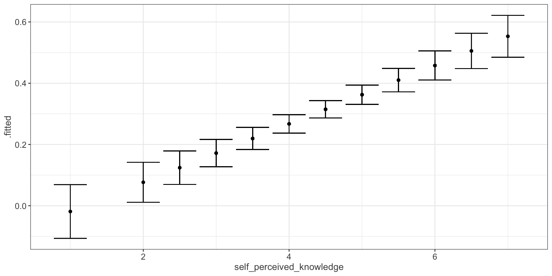
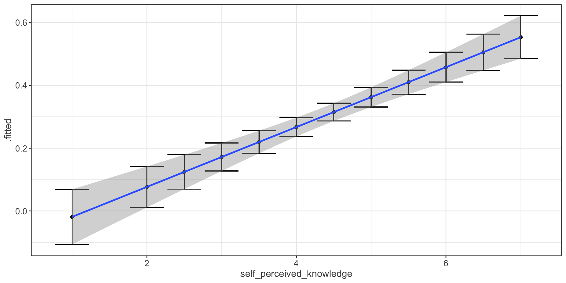
Compare mean estimate for self-perceived knowledge based on regression vs binning

Code

p1 = ggplot(expertise, aes(x=self_perceived_knowledge, y=overclaiming_proportion)) +
      geom_point() +   
  geom_smooth(method=lm,   # Add linear regression line
                se=TRUE) +
  scale_y_continuous(limits = c(-.12, 1.1))
p2 = expertise %>%
  mutate(self_perceived_knowledge = cut_interval(self_perceived_knowledge, length = 1)) %>%
  group_by(self_perceived_knowledge) %>%
  summarize(m = mean(overclaiming_proportion), 
          s = sd(overclaiming_proportion), 
          n = n(),
          se = s/sqrt(n),
          cv = qt(p = .975, df = n-2),
          moe = se*cv) %>%
  ggplot(aes(x = self_perceived_knowledge, y = m)) +
  geom_bar(stat = "identity") +
  geom_errorbar(aes(ymin = m-moe, ymax = m+moe)) +
  scale_y_continuous("overclaiming_proportion", limits = c(-.12, 1.1))

ggpubr::ggarrange(p1, p2, align = "v")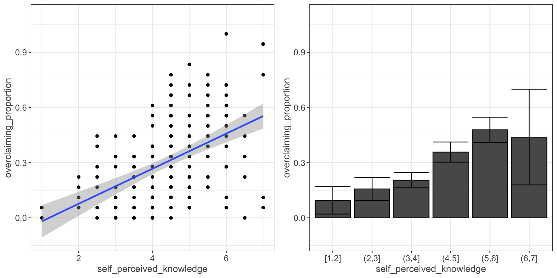

Confidence Bands

\[ \hat{Y}_i\pm t_{critical} * s_{Y|X}*\sqrt{\frac {1}{n}+\frac{(X_i-\bar{X})^2}{(n-1)s_{X}^2}}\] ### Prediction bands

\[\hat{Y}_i\pm t_{critical} * s_{Y|X}*\sqrt{1+ \frac {1}{n}+\frac{(X_i-\bar{X})^2}{(n-1)s_{X}^2}}\]

Prediction bands

• predicting an individual \(i's\) score, not the \(\hat{Y}\) for a particular level of X. (A new \(Y_i\) given \(X_i\), rather than \(\bar{Y}\) given \(X_i\) )

• Because there is greater variation in predicting an individual value rather than a mean, the prediction band is greater

• Combines unknown variability of the estimated mean \((\text{as reflected in }se_b)\) with peoples’ scores around mean \((\text{standard error of the estimate }, s_{Y|X})\)

Code

temp_var <- predict(fit.1, interval="prediction")
new_df <- cbind(expertise, temp_var)
pred <- ggplot(new_df, aes(x=self_perceived_knowledge, y=overclaiming_proportion))+
       geom_point() +   
  geom_smooth(method=lm,se=TRUE) +
 geom_ribbon(aes(ymin = lwr, ymax = upr), 
               fill = "blue", alpha = 0.1) +
  theme_bw(base_size = 20)

pred

Next time

The general linear model