General Linear Model
Last time
Wrap up univariate regression
Confidence and prediction bands
Today
General linear model
Models
Thus far you have used t-tests, correlations, and regressions to test basic questions about the world.
These types of tests can be thought of as a model for how you think “the world works”
Our DV (Y) is what we are trying to understand
We hypothesize it has some relationship with your IV(s) (Xs)
\[Y_i = b_0 + b_1X_i + e_i\]
General linear model
This model (equation) can be very simple as in a treatment/control experiment. It can be very complex in terms of trying to understand something like academic achievement
The majority of our models fall under the umbrella of a general(ized) linear model
General linear model
The general linear model is a family of models that assume the relationship between your DV and IV(s) is linear and additive, and that your residuals* are normally distributed.
This is a subset of the generalized linear model which allows for non-linear associations and non-normally distributed outcomes.
All models imply our theory about how the data are generated (i.e., how the world works)
Example
traffic = read.csv("https://raw.githubusercontent.com/uopsych/psy612/master/data/traffic.csv")
glimpse(traffic)
Rows: 280
Columns: 3
$ id <int> 1, 2, 3, 4, 5, 6, 7, 8, 9, 10, 11, 12, 13, 14, 15, 16, 17…
$ tx <int> 1, 1, 1, 1, 1, 1, 0, 0, 0, 1, 1, 0, 0, 0, 0, 0, 0, 0, 0, …
$ traffic.risk <dbl> 1.857143, 1.000000, 3.285714, 2.000000, 2.428571, 3.28571… vars n mean sd min max range se
id 1 280 140.50 80.97 1 280.00 279.00 4.84
tx 2 274 0.62 0.49 0 1.00 1.00 0.03
traffic.risk 3 272 2.35 0.81 1 4.71 3.71 0.05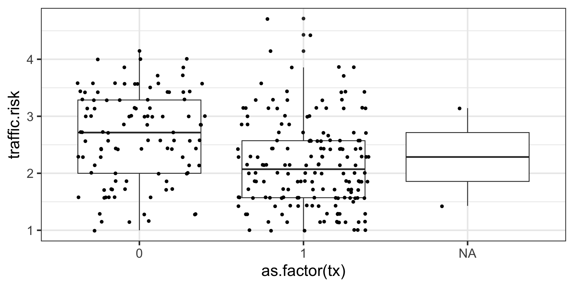
example
example
    Two Sample t-test

data:  traffic.risk by tx
t = 4.9394, df = 268, p-value = 1.381e-06
alternative hypothesis: true difference in means between group 0 and group 1 is not equal to 0
95 percent confidence interval:
 0.2893360 0.6728755
sample estimates:
mean in group 0 mean in group 1
       2.650641        2.169535
example
example
    Pearson's product-moment correlation

data:  traffic.risk and tx
t = -4.9394, df = 268, p-value = 1.381e-06
alternative hypothesis: true correlation is not equal to 0
95 percent confidence interval:
 -0.3946279 -0.1755371
sample estimates:
     cor
-0.28886
example
example
example cont
example cont
Call:
lm(formula = traffic.risk ~ tx, data = traffic)

Residuals:
     Min       1Q   Median       3Q      Max
-1.65064 -0.59811 -0.02668  0.54475  2.54475

Coefficients:
            Estimate Std. Error t value Pr(>|t|)
(Intercept)  2.65064    0.07637  34.707  < 2e-16 ***
tx          -0.48111    0.09740  -4.939 1.38e-06 ***
---
Signif. codes:  0 '***' 0.001 '**' 0.01 '*' 0.05 '.' 0.1 ' ' 1

Residual standard error: 0.7789 on 268 degrees of freedom
  (10 observations deleted due to missingness)
Multiple R-squared:  0.08344,   Adjusted R-squared:  0.08002
F-statistic:  24.4 on 1 and 268 DF,  p-value: 1.381e-06
example summary
Same p-values for each test; same SS; same test!
correlation gives you an effect size \((r)\) and \(df\)
t-test gives you a \(t\) & \(df\) (output may give you group \(M\) and \(s\))
ANOVA gives you an \(F\) (and \(SS\)s)
linear model (regression) gives you an equation in addition to \(F\) and \(SS\)
t-test as regression
\[Y_i = b_{0} + b_{1}X_i + e_i\]
\[\text{traffic risk}_i = b_{0} + b_{1}\text{tx}_i + e_i\]
Each individual (county) has a unique Y value, X value, and residual
The model only has a single \(b_{0}\) and \(b_{1}\) term.
- \(b_{0}\) is the intercept
- \(b_{1}\) quantifies the relationship between IV and the DV.
What do the estimates tell us?
NA [...]
Coefficients:
            Estimate Std. Error t value Pr(>|t|)
(Intercept)  2.65064    0.07637  34.707  < 2e-16 ***
tx          -0.48111    0.09740  -4.939 1.38e-06 ***
NA [...]
 Descriptive statistics by group
group: 0
   vars   n mean   sd median trimmed  mad min  max range  skew kurtosis   se
X1    1 104 2.65 0.79   2.71    2.67 0.95   1 4.14  3.14 -0.22    -0.96 0.08
------------------------------------------------------------
group: 1
   vars   n mean   sd median trimmed  mad min  max range skew kurtosis   se
X1    1 166 2.17 0.77   2.07    2.12 0.74   1 4.71  3.71 0.67     0.06 0.06
How to interpret regression estimates
Intercept is the mean of group of variable tx that is coded 0
Regression coefficient is the difference in means between the groups (i.e., slope)
Code
ggplot(traffic %>% filter(!is.na(tx))) +
  aes(x = as.factor(tx), y = traffic.risk) +
  stat_summary(geom="bar", fun=mean, aes(fill = as.factor(tx))) +
  geom_jitter(height = 0, width = .1) +
  stat_summary(geom="errorbar", fun.data=mean_cl_normal,
                 fun.args=list(conf.int=0.95), width = .5)+
  ylim(0,5)+
  guides(fill = F) +
  theme_bw(base_size = 20)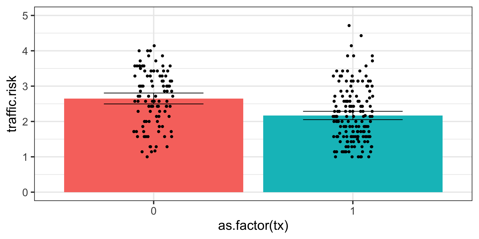
How to interpret regression estimates
Intercept \((b_0)\) signifies the level of Y when your model IVs (Xs) are zero
Regression \((b_1)\) signifies the difference for a one unit change in your X
as with last semester you have estimates (like \(\bar{X}\)) and standard errors, which you can then ask whether they are likely assuming a null or create a CI
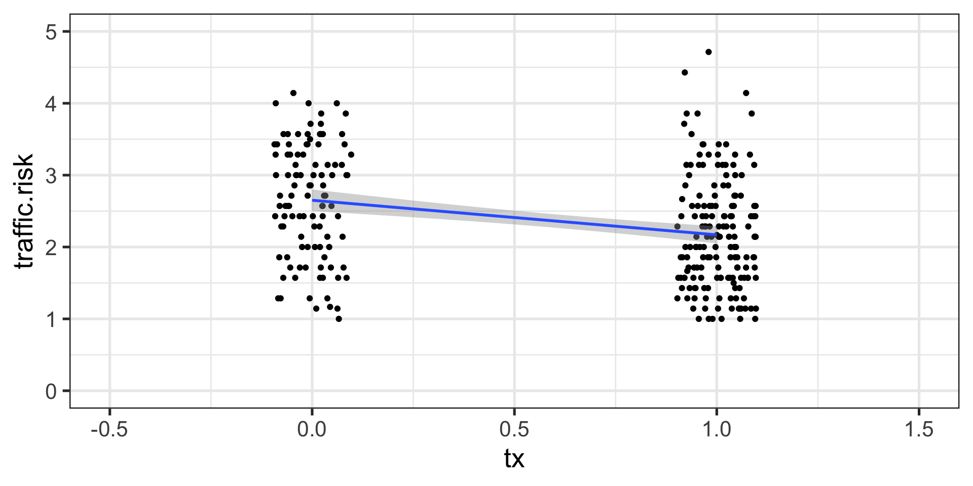
t-test as regression
Regression coefficients are another way of presenting the expected means of each group, but instead of \(M_1\) and \(M_2\), we’re given \(M_1\) and \(\Delta\) or the difference.
Now let’s compare the inferential test of the two.
Call:
lm(formula = traffic.risk ~ tx, data = traffic)

Residuals:
     Min       1Q   Median       3Q      Max
-1.65064 -0.59811 -0.02668  0.54475  2.54475

Coefficients:
            Estimate Std. Error t value Pr(>|t|)
(Intercept)  2.65064    0.07637  34.707  < 2e-16 ***
tx          -0.48111    0.09740  -4.939 1.38e-06 ***
---
Signif. codes:  0 '***' 0.001 '**' 0.01 '*' 0.05 '.' 0.1 ' ' 1

Residual standard error: 0.7789 on 268 degrees of freedom
  (10 observations deleted due to missingness)
Multiple R-squared:  0.08344,   Adjusted R-squared:  0.08002
F-statistic:  24.4 on 1 and 268 DF,  p-value: 1.381e-06
    Two Sample t-test

data:  traffic.risk by tx
t = 4.9394, df = 268, p-value = 1.381e-06
alternative hypothesis: true difference in means between group 0 and group 1 is not equal to 0
95 percent confidence interval:
 0.2893360 0.6728755
sample estimates:
mean in group 0 mean in group 1
       2.650641        2.169535
Statistical Inference
The p-values for the two tests are the same, because they are the same test.
The probability distribution may differ… sort of. Recall that all these distributions are derived from the standard normal.
- t-test uses a t-distribution
- regression uses an F-distribution for the omnibus test
- regression uses a t-distribution for the test of the coefficients
Statistical Inference
In the case of a single binary predictor, the t-statistic for the t-test will be identical to the t-statistic of the regression coefficient test.
The F-statistic of the omnibus test will be the t-statistic squared: \(F = t^2\)
library(here)
expertise = read.csv("https://raw.githubusercontent.com/uopsych/psy612/master/data/expertise.csv")
cor.test(expertise$self_perceived_knowledge, expertise$overclaiming_proportion, use = "pairwise")
    Pearson's product-moment correlation

data:  expertise$self_perceived_knowledge and expertise$overclaiming_proportion
t = 7.762, df = 200, p-value = 4.225e-13
alternative hypothesis: true correlation is not equal to 0
95 percent confidence interval:
 0.3675104 0.5806336
sample estimates:
      cor
0.4811502
Call:
lm(formula = overclaiming_proportion ~ self_perceived_knowledge,
    data = expertise)

Residuals:
     Min       1Q   Median       3Q      Max
-0.50551 -0.15610  0.00662  0.12167  0.54215

Coefficients:
                         Estimate Std. Error t value Pr(>|t|)
(Intercept)              -0.11406    0.05624  -2.028   0.0439 *
self_perceived_knowledge  0.09532    0.01228   7.762 4.22e-13 ***
---
Signif. codes:  0 '***' 0.001 '**' 0.01 '*' 0.05 '.' 0.1 ' ' 1

Residual standard error: 0.2041 on 200 degrees of freedom
Multiple R-squared:  0.2315,    Adjusted R-squared:  0.2277
F-statistic: 60.25 on 1 and 200 DF,  p-value: 4.225e-13
Call:
lm(formula = self_perceived_knowledge ~ overclaiming_proportion,
    data = expertise)

Residuals:
    Min      1Q  Median      3Q     Max
-2.8150 -0.6761  0.0103  0.7305  3.1850

Coefficients:
                        Estimate Std. Error t value Pr(>|t|)
(Intercept)               3.6801     0.1206  30.515  < 2e-16 ***
overclaiming_proportion   2.4288     0.3129   7.762 4.22e-13 ***
---
Signif. codes:  0 '***' 0.001 '**' 0.01 '*' 0.05 '.' 0.1 ' ' 1

Residual standard error: 1.03 on 200 degrees of freedom
Multiple R-squared:  0.2315,    Adjusted R-squared:  0.2277
F-statistic: 60.25 on 1 and 200 DF,  p-value: 4.225e-13
Regression models provide all the same information as the t-test or correlation. But they provide additional information.
Regression omnibus test are the same as t-test or correlation tests, even the same as ANOVAs. But the coefficient tests give you additional information, like intercepts, and make it easier to calculate predicted values and to assess relative fit.
Predictions
predictions \(\hat{Y}\) are of the form of \(E(Y|X)\)
They are created by simply plugging a persons X’s into the created model
If you have b’s and have X’s you can create a prediction
\(\large \hat{Y}_{i} = 2.6506410 + -0.4811057X_{i}\)
Call:
lm(formula = traffic.risk ~ tx, data = traffic)

Residuals:
     Min       1Q   Median       3Q      Max
-1.65064 -0.59811 -0.02668  0.54475  2.54475

Coefficients:
            Estimate Std. Error t value Pr(>|t|)
(Intercept)  2.65064    0.07637  34.707  < 2e-16 ***
tx          -0.48111    0.09740  -4.939 1.38e-06 ***
---
Signif. codes:  0 '***' 0.001 '**' 0.01 '*' 0.05 '.' 0.1 ' ' 1

Residual standard error: 0.7789 on 268 degrees of freedom
  (10 observations deleted due to missingness)
Multiple R-squared:  0.08344,   Adjusted R-squared:  0.08002
F-statistic:  24.4 on 1 and 268 DF,  p-value: 1.381e-06
Predictions
Unless you’ve collected a new dataset, you can’t really assess the accuracy of predictions. Instead, we evaluate the fit to the data used to create the model. We want \(\hat{Y}_i\) to be close to our actual data for each person \((Y_{i})\)
The difference between the actual data and our guess \((Y_{i} - \hat{Y}_{i} = e)\) is the residual, how far we are “off”. This tells us how good our fit is.
You can have the same estimates for two models but completely different fit.
Which one has better fit?
Code
twogroup_fun = function(nrep = 100, b0 = 6, b1 = -2, sigma = 1) {
     ngroup = 2
     group = rep( c("group1", "group2"), each = nrep)
     eps = rnorm(ngroup*nrep, 0, sigma)
     traffic = b0 + b1*(group == "group2") + eps
     growthfit = lm(traffic ~ group)
     growthfit
}


twogroup_fun2 = function(nrep = 100, b0 = 6, b1 = -2, sigma = 2) {
     ngroup = 2
     group = rep( c("group1", "group2"), each = nrep)
     eps = rnorm(ngroup*nrep, 0, sigma)
     traffic = b0 + b1*(group == "group2") + eps
     growthfit = lm(traffic ~ group)
     growthfit
}

set.seed(16)
library(broom)
lm1 <- augment(twogroup_fun())

set.seed(16)
lm2 <- augment(twogroup_fun2())

plot1<- ggplot(lm1) +
  aes(x = group, y = traffic) +
  geom_boxplot() + geom_jitter() + ylim(-1, 11)+ theme_bw(base_size = 20)

plot2<- ggplot(lm2) +
  aes(x = group, y = traffic) +
  geom_boxplot() + geom_jitter() + ylim(-1, 11)+ theme_bw(base_size = 20)


library(gridExtra)
 grid.arrange(plot1, plot2, ncol=2)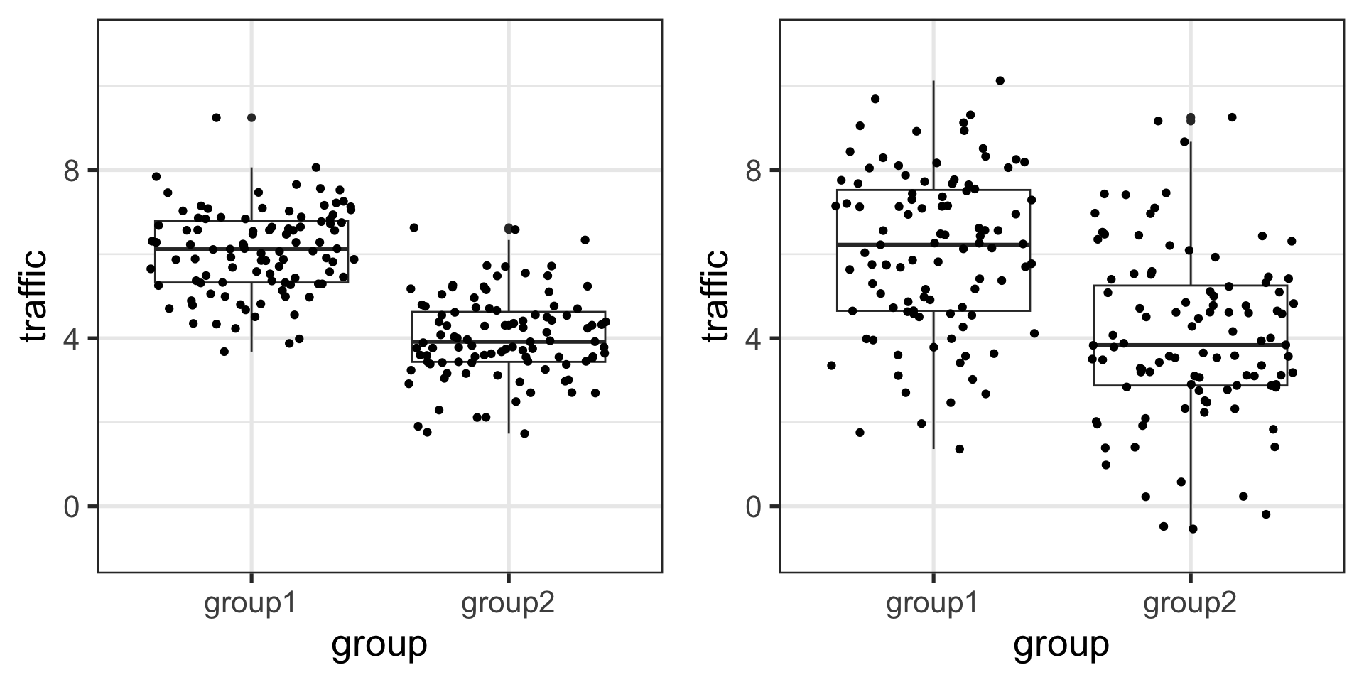
Calculating fitted and predicted values
\[\hat{Y}_{i} = b_{0} + b_{1}X_{i}\]
\[Y_{i} = b_{0} + b_{1}X_{i} +e_{i}\]
\[Y_{i} - \hat{Y}_{i} = e\]
Plug in numbers and calculate County 3’s fitted and residual scores without explicitly asking for lm object residuals and fitted values?
\(\large \hat{Y}_{i} = 2.65 + -0.48X_{i}\)
Predicting with new data
A tangent about “predict”
“Predict” can refer to multiple things in a regression analyses.
- Fitted values of data used to estimate model \((\hat{Y}_i)\)
- Fitted values of new data (machine learning)
- The range of possible/expected \(Y\)’s for any given X (prediction interval)
A tangent about “predict”
Some people are really picky about when you can and cannot use this term.
- I am not one of those people.
- Pick a definition, explain it, and be consistent.
A tangent about “predict”
Code
ci_est = predict(mod.1,
        newdata = new.df,
        interval = "confidence") %>%
  as.data.frame() %>%
  mutate(tx = c(0,1),
         interval = "confidence")

pred_est = predict(mod.1,
        newdata = new.df,
        interval = "prediction") %>%
  as.data.frame() %>%
  mutate(tx = c(0,1),
         interval = "prediction")

full_join(ci_est, pred_est) %>%
  ggplot(aes(x = tx, y = fit)) +
  geom_errorbar(aes(ymin = lwr, ymax = upr, color = interval)) +
  geom_point() +
  scale_x_continuous("tx", breaks = c(0,1)) +
  scale_y_continuous(expression(hat(Y))) +
  theme_pubr()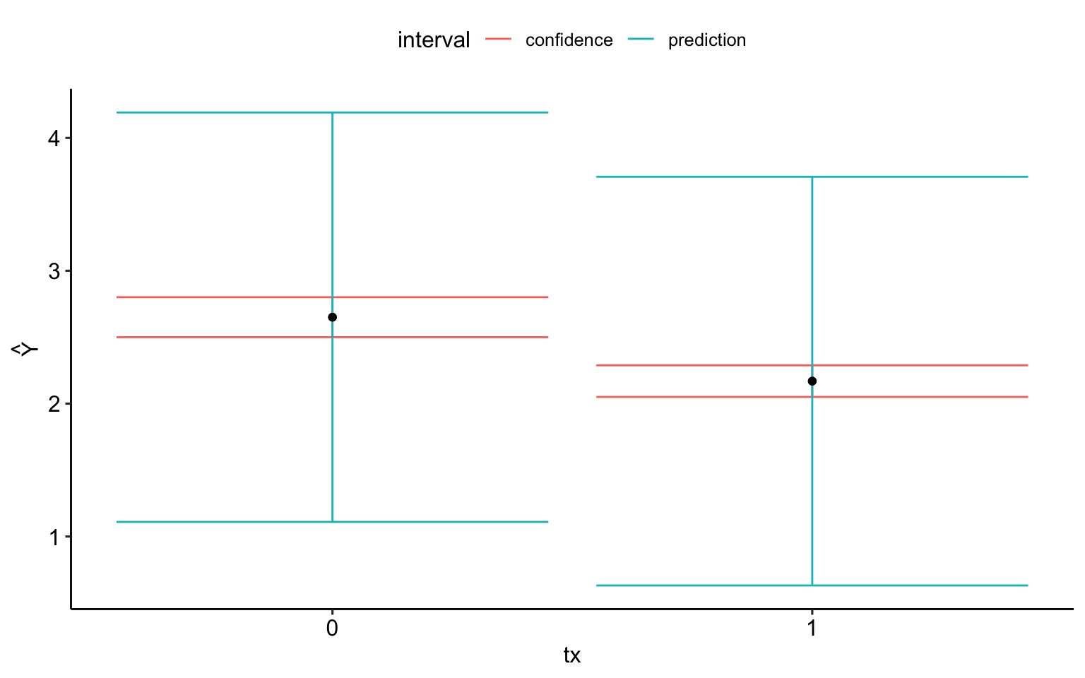
Back to statistical inference
To evaluate our model, we have to compare our guesses to some alternative guesses to see if we are doing well or not.
What is our best guess (i.e., prediction) if we didn’t collect any data?
\[\hat{Y} = \bar{Y}\]
Back to statistical inference
Regression can be thought of as: is \(E(Y|X)\) better than \(E(Y)\)?
To the extent that we can generate different guesses of Y based on the values of the IVs, our model is doing well. Said differently, the closer our model is to the “actual” data generating model, our guesses \((\hat{Y})\) will be closer to our actual data \((Y)\)
Partitioning variation
\[\sum (Y - \bar{Y})^2 = \sum (\hat{Y} -\bar{Y})^2 + \sum(Y - \hat{Y})^2\]
SS total = SS between + SS within
SS total = SS regression + SS residual (or error)
Technically, we haven’t gotten to ANOVA yet, but you can run and interpret an ANOVA with no problems given what we’ve talked about already.
summary
The general linear model is a way of mathematically building a theoretical model and testing it with data. GLMs assume the relationship between your IVs and DV is linear
- t-tests, ANOVAs, even \(\chi^2\) tests are special cases of the general linear model. The benefit to looking at these tests through the perspective of a linear model is that it provides us with all the information of those tests and more! Plus it provides a more systematic way at 1) building and testing your theoretical model and 2) comparing between alternative theoretical models
I made this meme for our stats class last week and I thought you might like to see it. pic.twitter.com/ecnfsXHvey
— Stuart Ritchie (@StuartJRitchie) October 27, 2019
Next time
Part- and partial correlations