Multiple regression

Part 2

Last time

• Introduction to multiple regression
• Interpreting coefficient estimates
• Estimating model fit
• Significance tests (omnibus and coefficients)

Today

• Tolerance
• Hierarchical regression/model comparison

Example from Thursday

library(here); library(tidyverse); library(kableExtra)
support_df = read.csv(here("data/support.csv")) 
psych::describe(support_df, fast = T)

                vars  n mean   sd  min  max range   se
give_support       1 78 4.99 1.07 2.77 7.43  4.66 0.12
receive_support    2 78 7.88 0.85 5.81 9.68  3.87 0.10
relationship       3 78 5.85 0.86 3.27 7.97  4.70 0.10

mr.model <- lm(relationship ~ receive_support + give_support, data = support_df)
summary(mr.model)

Call:
lm(formula = relationship ~ receive_support + give_support, data = support_df)

Residuals:
     Min       1Q   Median       3Q      Max 
-2.26837 -0.40225  0.07701  0.42147  1.76074 

Coefficients:
                Estimate Std. Error t value Pr(>|t|)   
(Intercept)      2.07212    0.81218   2.551  0.01277 * 
receive_support  0.37216    0.11078   3.359  0.00123 **
give_support     0.17063    0.08785   1.942  0.05586 . 
---
Signif. codes:  0 '***' 0.001 '**' 0.01 '*' 0.05 '.' 0.1 ' ' 1

Residual standard error: 0.7577 on 75 degrees of freedom
Multiple R-squared:  0.2416,    Adjusted R-squared:  0.2214 
F-statistic: 11.95 on 2 and 75 DF,  p-value: 3.128e-05

Standard error of regression coefficient

In the case of univariate regression:

\[\Large se_{b} = \frac{s_{Y}}{s_{X}}{\sqrt{\frac {1-r_{xy}^2}{n-2}}}\]

In the case of multiple regression:

\[\Large se_{b} = \frac{s_{Y}}{s_{X}}{\sqrt{\frac {1-R_{Y\hat{Y}}^2}{n-p-1}}} \sqrt{\frac {1}{1-R_{i.jkl...p}^2}}\]

• As N increases…
• As variance explained increases…

\[se_{b} = \frac{s_{Y}}{s_{X}}{\sqrt{\frac {1-R_{Y\hat{Y}}^2}{n-p-1}}} \sqrt{\frac {1}{1-R_{i.jkl...p}^2}}\]

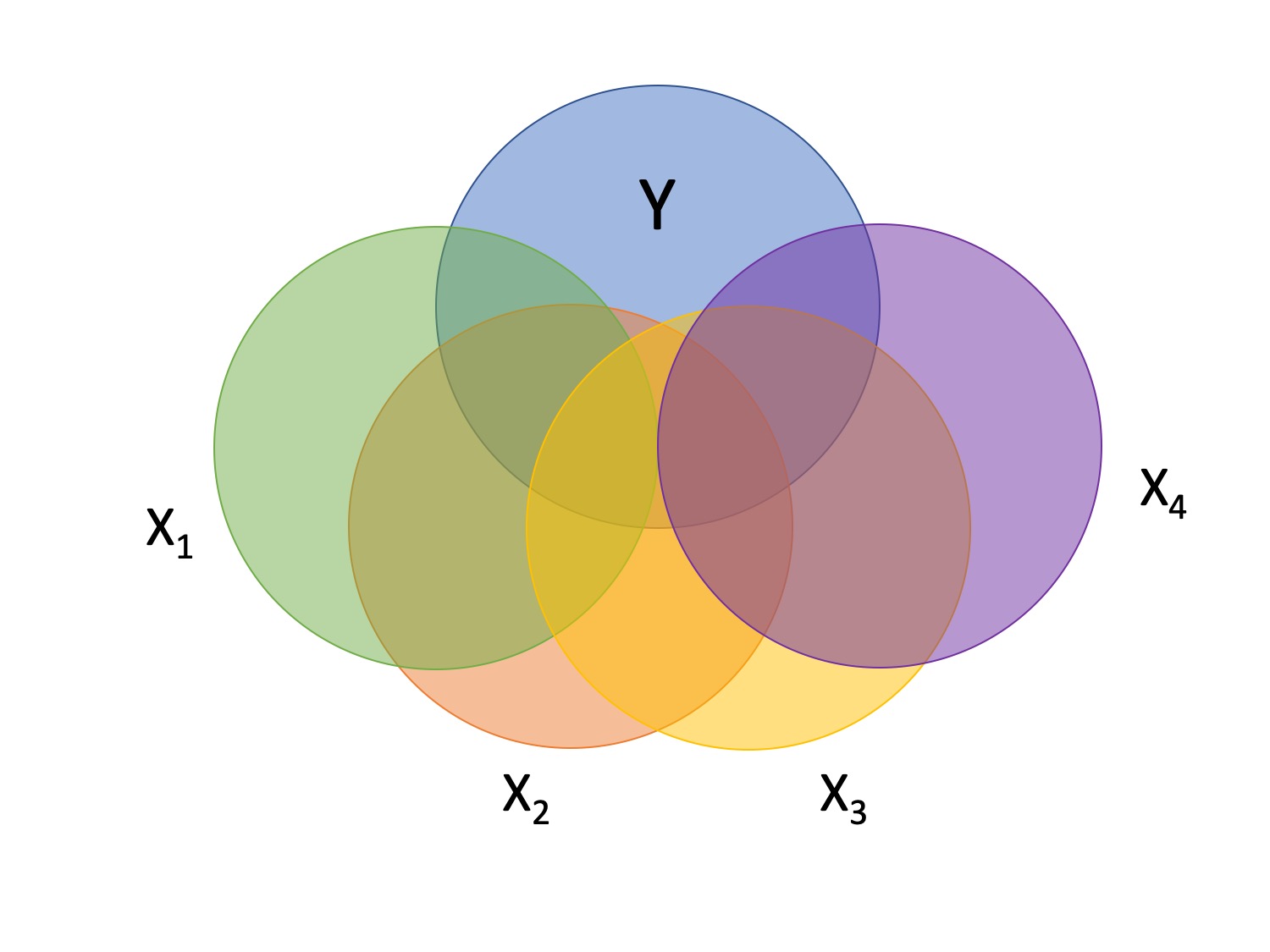
Tolerance

\[1-R_{i.jkl...p}^2\]

• Proportion of \(X_i\) that does not overlap with other predictors.
  • Bounded by 0 and 1

• Large tolerance (little overlap) means standard error will be small.
  
• what does this mean for including a lot of variables in your model?

Tolerance in R

library(olsrr)

ols_vif_tol(mr.model)

        Variables Tolerance      VIF
1 receive_support 0.8450326 1.183386
2    give_support 0.8450326 1.183386

Why are tolerance values identical here?

Suppression

Normally our standardized partial regression coefficients fall between 0 and \(r_{Y1}\). However, it is possible for \(b^*_{Y1}\) to be larger than \(r_{Y1}\). We refer to this phenomenon as suppression.

• A non-significant \(r_{Y1}\) can become a significant \(b^*_{Y1}\) when additional variables are added to the model.

• A positive \(r_{Y1}\) can become a negative and significant \(b^*_{Y1}\).

stress_df = read.csv(here("data/stress.csv")) %>% dplyr::select(-id, -group)

cor(stress_df) %>% round(2)

        Anxiety Stress Support
Anxiety    1.00  -0.05   -0.55
Stress    -0.05   1.00    0.52
Support   -0.55   0.52    1.00

lm(Stress ~ Anxiety, data = stress_df) %>% summary

Call:
lm(formula = Stress ~ Anxiety, data = stress_df)

Residuals:
   Min     1Q Median     3Q    Max 
-4.580 -1.338  0.130  1.047  4.980 

Coefficients:
            Estimate Std. Error t value Pr(>|t|)    
(Intercept)  5.45532    0.56017   9.739   <2e-16 ***
Anxiety     -0.03616    0.06996  -0.517    0.606    
---
Signif. codes:  0 '***' 0.001 '**' 0.01 '*' 0.05 '.' 0.1 ' ' 1

Residual standard error: 1.882 on 116 degrees of freedom
Multiple R-squared:  0.002297,  Adjusted R-squared:  -0.006303 
F-statistic: 0.2671 on 1 and 116 DF,  p-value: 0.6063

lm(Stress ~ Anxiety + Support, data = stress_df) %>% summary

Call:
lm(formula = Stress ~ Anxiety + Support, data = stress_df)

Residuals:
    Min      1Q  Median      3Q     Max 
-4.1958 -0.8994 -0.1370  0.9990  3.6995 

Coefficients:
            Estimate Std. Error t value Pr(>|t|)    
(Intercept) -0.31587    0.85596  -0.369 0.712792    
Anxiety      0.25609    0.06740   3.799 0.000234 ***
Support      0.40618    0.05115   7.941 1.49e-12 ***
---
Signif. codes:  0 '***' 0.001 '**' 0.01 '*' 0.05 '.' 0.1 ' ' 1

Residual standard error: 1.519 on 115 degrees of freedom
Multiple R-squared:  0.3556,    Adjusted R-squared:  0.3444 
F-statistic: 31.73 on 2 and 115 DF,  p-value: 1.062e-11

Suppression

Recall that the partial regression coefficient is calculated:

\[\large b^*_{Y1.2}=\frac{r_{Y1}-r_{Y2}r_{12}}{1-r^2_{12}}\]

Is suppression meaningful?

Imagine a scenario when X2 and Y are uncorrelated and X2 is correlated with X1.

(Draw Venn diagram of this)

Second part of numerator becomes 0 Bottom part gets smaller Bigger value

Hierarchical regression/Model comparison

library(tidyverse)
happy_d <- read_csv('http://static.lib.virginia.edu/statlab/materials/data/hierarchicalRegressionData.csv')
happy_d$gender = ifelse(happy_d$gender == "Female", 1, 0)
library(psych)
describe(happy_d, fast = T)

          vars   n  mean   sd min max range   se
happiness    1 100  4.46 1.56   1   9     8 0.16
age          2 100 25.37 1.97  20  30    10 0.20
gender       3 100  0.39 0.49   0   1     1 0.05
friends      4 100  6.94 2.63   1  14    13 0.26
pets         5 100  1.10 1.18   0   5     5 0.12

mr.model <- lm(happiness ~ age + gender + friends + pets, data = happy_d)
summary(mr.model)

Call:
lm(formula = happiness ~ age + gender + friends + pets, data = happy_d)

Residuals:
    Min      1Q  Median      3Q     Max 
-3.0556 -1.0183 -0.1109  0.8832  3.5911 

Coefficients:
            Estimate Std. Error t value Pr(>|t|)   
(Intercept)  5.64273    1.93194   2.921  0.00436 **
age         -0.11146    0.07309  -1.525  0.13057   
gender       0.14267    0.31157   0.458  0.64806   
friends      0.17134    0.05491   3.120  0.00239 **
pets         0.36391    0.13044   2.790  0.00637 **
---
Signif. codes:  0 '***' 0.001 '**' 0.01 '*' 0.05 '.' 0.1 ' ' 1

Residual standard error: 1.427 on 95 degrees of freedom
Multiple R-squared:  0.1969,    Adjusted R-squared:  0.1631 
F-statistic: 5.822 on 4 and 95 DF,  p-value: 0.0003105

Review here: * Omnibus test * Coefficient of determination * Adjust R squared * Resid standard error * Coefficient estimates

Methods for entering variables

Simultaneous: Enter all of your IV’s in a single model.

\[\large Y = b_0 + b_1X_1 + b_2X_2 + b_3X_3\]

• The benefits to using this method is that it reduces researcher degrees of freedom, is a more conservative test of any one coefficient, and often the most defensible action (unless you have specific theory guiding a hierarchical approach).

Methods for entering variables

Hierarchically: Build a sequence of models in which every successive model includes one more (or one fewer) IV than the previous. \[\large Y = b_0 + e\] \[\large Y = b_0 + b_1X_1 + e\] \[\large Y = b_0 + b_1X_1 + b_2X_2 + e\] \[\large Y = b_0 + b_1X_1 + b_2X_2 + b_3X_3 + e\]

This is known as hierarchical regression. (Note that this is different from Hierarchical Linear Modelling or HLM [which is often called Multilevel Modeling or MLM].) Hierarchical regression is a subset of model comparison techniques.

Hierarchical regression / Model Comparison

Model comparison: Comparing how well two (or more) models fit the data in order to determine which model is better.

If we’re comparing nested models by incrementally adding or subtracting variables, this is known as hierarchical regression.

• Multiple models are calculated

• Each predictor (or set of predictors) is assessed in terms of what it adds (in terms of variance explained) at the time it is entered

• Order is dependent on an a priori hypothesis

\(R^2\) change

• distributed as an F

\[F(p.new, N - 1 - p.all) = \frac {R_{m.2}^2- R_{m.1}^2} {1-R_{m.2}^2} (\frac {N-1-p.all}{p.new})\]

• can also be written in terms of SSresiduals

Model comparison

• The basic idea is asking how much variance remains unexplained in our model. This “left over” variance can be contrasted with an alternative model/hypothesis. We can ask does adding a new predictor variable help explain more variance or should we stick with a parsimonious model.

• Every test of an omnibus model is implicitly a model comparisons, typically of your fitted model with the nil model (no slopes). This framework allows you to be more flexible and explicit.

fit.0 <- lm(happiness ~ 1,
            data = happy_d)

summary(fit.0)

Call:
lm(formula = happiness ~ 1, data = happy_d)

Residuals:
   Min     1Q Median     3Q    Max 
 -3.46  -0.71  -0.46   0.54   4.54 

Coefficients:
            Estimate Std. Error t value Pr(>|t|)    
(Intercept)    4.460      0.156   28.59   <2e-16 ***
---
Signif. codes:  0 '***' 0.001 '**' 0.01 '*' 0.05 '.' 0.1 ' ' 1

Residual standard error: 1.56 on 99 degrees of freedom

fit.1 <- lm(happiness ~ age,
            data = happy_d)
summary(fit.1)

Call:
lm(formula = happiness ~ age, data = happy_d)

Residuals:
    Min      1Q  Median      3Q     Max 
-3.7615 -0.9479 -0.1890  0.7792  4.3657 

Coefficients:
            Estimate Std. Error t value Pr(>|t|)    
(Intercept)  7.68763    2.00570   3.833 0.000224 ***
age         -0.12722    0.07882  -1.614 0.109735    
---
Signif. codes:  0 '***' 0.001 '**' 0.01 '*' 0.05 '.' 0.1 ' ' 1

Residual standard error: 1.547 on 98 degrees of freedom
Multiple R-squared:  0.02589,   Adjusted R-squared:  0.01595 
F-statistic: 2.605 on 1 and 98 DF,  p-value: 0.1097

anova(fit.0)

Analysis of Variance Table

Response: happiness
          Df Sum Sq Mean Sq F value Pr(>F)
Residuals 99 240.84  2.4327               

anova(fit.1)

Analysis of Variance Table

Response: happiness
          Df  Sum Sq Mean Sq F value Pr(>F)
age        1   6.236  6.2364  2.6051 0.1097
Residuals 98 234.604  2.3939               

anova(fit.1, fit.0)

Analysis of Variance Table

Model 1: happiness ~ age
Model 2: happiness ~ 1
  Res.Df    RSS Df Sum of Sq      F Pr(>F)
1     98 234.60                           
2     99 240.84 -1   -6.2364 2.6051 0.1097

Model Comparisons

• This example of model comparisons is redundant with nil/null hypotheses and coefficient tests of slopes in univariate regression.

• Let’s expand this to the multiple regression case model.

Model comparisons

m.2 <- lm(happiness ~ age + gender, data = happy_d)
m.3 <- lm(happiness ~ age + gender + pets, data = happy_d)
m.4 <- lm(happiness ~ age + gender + friends + pets, data = happy_d)
anova(m.2, m.3, m.4)

...
Analysis of Variance Table

Model 1: happiness ~ age + gender
Model 2: happiness ~ age + gender + pets
Model 3: happiness ~ age + gender + friends + pets
  Res.Df    RSS Df Sum of Sq       F   Pr(>F)   
1     97 233.97                                 
2     96 213.25  1    20.721 10.1769 0.001927 **
3     95 193.42  1    19.821  9.7352 0.002394 **
...

coef(summary(m.4))

              Estimate Std. Error    t value    Pr(>|t|)
(Intercept)  5.6427256 1.93193747  2.9207599 0.004361745
age         -0.1114606 0.07308612 -1.5250586 0.130566815
gender       0.1426730 0.31156820  0.4579192 0.648056200
friends      0.1713379 0.05491363  3.1201349 0.002394079
pets         0.3639113 0.13044467  2.7897749 0.006373887

change in \(R^2\)

summary(m.2)$r.squared

[1] 0.02854509

summary(m.3)$r.squared

[1] 0.1145794

summary(m.4)$r.squared

[1] 0.1968801

partitioning the variance

• It doesn’t make sense to ask how much variance a variable explains (unless you qualify the association)

\[R_{Y.1234...p}^2 = r_{Y1}^2 + r_{Y(2.1)}^2 + r_{Y(3.21)}^2 + r_{Y(4.321)}^2 + ...\]

• In other words: order matters!

What if we compare the first (2 predictors) and last model (4 predictors)?

anova(m.2, m.4)

Analysis of Variance Table

Model 1: happiness ~ age + gender
Model 2: happiness ~ age + gender + friends + pets
  Res.Df    RSS Df Sum of Sq      F    Pr(>F)    
1     97 233.97                                  
2     95 193.42  2    40.542 9.9561 0.0001187 ***
---
Signif. codes:  0 '***' 0.001 '**' 0.01 '*' 0.05 '.' 0.1 ' ' 1

Model comparison can thus be very useful for testing the explained variance attributable to a set of predictors, not just one.

For example, if we’re interested in explaining variance in cognitive decline, perhaps we build a model comparison testing:

• Set 1: Demographic variables (age, gender, education, income)
• Set 2: Physical health (exercise, chronic illness, smoking, flossing)
• Set 3: Social factors (relationship quality, social network size)

Categorical predictors

One of the benefits of using regression (instead of partial correlations) is that it can handle both continuous and categorical predictors and allows for using both in the same model.

Categorical predictors with more than two levels are broken up into several smaller variables. In doing so, we take variables that don’t have any inherent numerical value to them (i.e., nominal and ordinal variables) and ascribe meaningful numbers that allow for us to calculate meaningful statistics.

You can choose just about any numbers to represent your categorical variable. However, there are several commonly used methods that result in very useful statistics.

Dummy coding

In dummy coding, one group is selected to be a reference group. From your single nominal variable with K levels, \(K-1\) dummy code variables are created; for each new dummy code variable, one of the non-reference groups is assigned 1; all other groups are assigned 0.

Occupation	D1	D2
Engineer	0	0
Teacher	1	0
Doctor	0	1

Person	Occupation	D1	D2
Billy	Engineer	0	0
Susan	Teacher	1	0
Michael	Teacher	1	0
Molly	Engineer	0	0
Katie	Doctor	0	1

Example

Following traumatic experiences, some people have flashbacks, which are also called “intrusive memories” and are characterized by involuntary images of aspects of the traumatic event. Research suggests that it may help to try to change the memory during reconsolidation, which occurs following the reactivation of a previously formed memory.

Because intrusive memories of trauma are often visual in nature, James and colleagues (2015) sought to explore whether completing a visuospatial task (e.g., tetris) while a memory is reconsolidating would interfere with the storage of that memory, and thereby reduce the frequency of subsequent intrusions.

Example

tetris = read.csv(here("data/james_e2.csv"), stringsAsFactors = T)
tetris = janitor::clean_names(tetris) %>% 
  rename(intrusions = days_one_to_seven_number_of_intrusions)
tetris = tetris %>% select(condition, intrusions)
summary(tetris)

                 condition    intrusions    
 Control              :18   Min.   : 0.000  
 Reactivation + Tetris:18   1st Qu.: 2.000  
 Reactivation Only    :18   Median : 3.000  
 Tetris Only          :18   Mean   : 3.931  
                            3rd Qu.: 5.000  
                            Max.   :16.000  

Let’s apply dummy coding to our example data. We’ll have to pick one of the groups to be our reference group, and then all other groups will have their own dummy code.

tetris = tetris %>%
  mutate(dummy_2 = ifelse(condition == "Reactivation + Tetris", 1, 0),
         dummy_3 = ifelse(condition == "Reactivation Only",     1, 0),
         dummy_4 = ifelse(condition == "Tetris Only",           1, 0)) 

Code

tetris %>%
  sample_n(size = 10) %>% 
  kable() %>% kable_classic()

condition	intrusions	dummy_2	dummy_3	dummy_4
Control	2	0	0	0
Control	0	0	0	0
Reactivation Only	6	0	1	0
Reactivation Only	7	0	1	0
Control	7	0	0	0
Reactivation Only	15	0	1	0
Control	6	0	0	0
Reactivation + Tetris	1	1	0	0
Reactivation Only	4	0	1	0
Reactivation Only	3	0	1	0

mod.1 = lm(intrusions ~ dummy_2 + dummy_3 + dummy_4, data = tetris)
summary(mod.1)

Call:
lm(formula = intrusions ~ dummy_2 + dummy_3 + dummy_4, data = tetris)

Residuals:
    Min      1Q  Median      3Q     Max 
-5.1111 -1.8889 -0.8333  1.1111 10.8889 

Coefficients:
            Estimate Std. Error t value Pr(>|t|)    
(Intercept)   5.1111     0.7485   6.828 2.89e-09 ***
dummy_2      -3.2222     1.0586  -3.044  0.00332 ** 
dummy_3      -0.2778     1.0586  -0.262  0.79381    
dummy_4      -1.2222     1.0586  -1.155  0.25231    
---
Signif. codes:  0 '***' 0.001 '**' 0.01 '*' 0.05 '.' 0.1 ' ' 1

Residual standard error: 3.176 on 68 degrees of freedom
Multiple R-squared:  0.1434,    Adjusted R-squared:  0.1056 
F-statistic: 3.795 on 3 and 68 DF,  p-value: 0.01409

Interpreting coefficients

When working with dummy codes, the intercept can be interpreted as the mean of the reference group.

\[\begin{aligned} \hat{Y} &= b_0 + b_1D_2 + b_2D_3 + b_3D_2 \\ \hat{Y} &= b_0 + b_1(0) + b_2(0) + b_3(0) \\ \hat{Y} &= b_0 \\ \hat{Y} &= \bar{Y}_{\text{Reference}} \end{aligned}\]

What do each of the slope coefficients mean?

From this equation, we can get the mean of every single group.

newdata = data.frame(dummy_2 = c(0,1,0,0),
                     dummy_3 = c(0,0,1,0),
                     dummy_4 = c(0,0,0,1))
predict(mod.1, newdata = newdata, se.fit = T)

$fit
       1        2        3        4 
5.111111 1.888889 4.833333 3.888889 

$se.fit
        1         2         3         4 
0.7485462 0.7485462 0.7485462 0.7485462 

$df
[1] 68

$residual.scale
[1] 3.175812

And the test of the coefficient represents the significance test of each group to the reference. This is an independent-samples t-test¹.

The test of the intercept is the one-sample t-test comparing the intercept to 0.

summary(mod.1)

...
            Estimate Std. Error t value Pr(>|t|)    
(Intercept)   5.1111     0.7485   6.828 2.89e-09 ***
dummy_2      -3.2222     1.0586  -3.044  0.00332 ** 
dummy_3      -0.2778     1.0586  -0.262  0.79381    
dummy_4      -1.2222     1.0586  -1.155  0.25231    
...

What if you wanted to compare groups 2 and 3?

tetris %>% 
  filter(condition %in% c("Control","Reactivation + Tetris")) %>% 
  t.test(intrusions ~ condition, data = ., var.equal = T)

    Two Sample t-test

data:  intrusions by condition
t = 2.9893, df = 34, p-value = 0.005167
alternative hypothesis: true difference in means between group Control and group Reactivation + Tetris is not equal to 0
95 percent confidence interval:
 1.031592 5.412852
sample estimates:
              mean in group Control mean in group Reactivation + Tetris 
                           5.111111                            1.888889 

1. Except for a few crucial differences: the standard error and degrees of freedom use all the data in the model, including those in groups 3 and 4.

tetris = tetris %>%
  mutate(dummy_1 = ifelse(condition == "Control",           1, 0),
         dummy_3 = ifelse(condition == "Reactivation Only", 1, 0),
         dummy_4 = ifelse(condition == "Tetris Only",       1, 0)) 
mod.2 = lm(intrusions ~ dummy_1 + dummy_3 + dummy_4, data = tetris)
summary(mod.2)

Call:
lm(formula = intrusions ~ dummy_1 + dummy_3 + dummy_4, data = tetris)

Residuals:
    Min      1Q  Median      3Q     Max 
-5.1111 -1.8889 -0.8333  1.1111 10.8889 

Coefficients:
            Estimate Std. Error t value Pr(>|t|)   
(Intercept)   1.8889     0.7485   2.523  0.01396 * 
dummy_1       3.2222     1.0586   3.044  0.00332 **
dummy_3       2.9444     1.0586   2.781  0.00700 **
dummy_4       2.0000     1.0586   1.889  0.06312 . 
---
Signif. codes:  0 '***' 0.001 '**' 0.01 '*' 0.05 '.' 0.1 ' ' 1

Residual standard error: 3.176 on 68 degrees of freedom
Multiple R-squared:  0.1434,    Adjusted R-squared:  0.1056 
F-statistic: 3.795 on 3 and 68 DF,  p-value: 0.01409

In all multiple regression models, we have to consider the correlations between the IVs, as highly correlated variables make it more difficult to detect significance of a particular X. One useful way to conceptualize the relationship between any two variables is “Does knowing someone’s score on \(X_1\) affect my guess for their score on \(X_2\)?”

Are dummy codes associated with a categorical predictor correlated or uncorrelated?

cor(tetris[,grepl("dummy", names(tetris))], use = "pairwise")

           dummy_2    dummy_3    dummy_4    dummy_1
dummy_2  1.0000000 -0.3333333 -0.3333333 -0.3333333
dummy_3 -0.3333333  1.0000000 -0.3333333 -0.3333333
dummy_4 -0.3333333 -0.3333333  1.0000000 -0.3333333
dummy_1 -0.3333333 -0.3333333 -0.3333333  1.0000000

Omnibus test

Doesn’t matter which set of dummy codes you use!

summary(mod.1)

...
F-statistic: 3.795 on 3 and 68 DF,  p-value: 0.01409
NA
...

summary(mod.2)

...
F-statistic: 3.795 on 3 and 68 DF,  p-value: 0.01409
NA
...

Next time…

Analysis of Variance (ANOVA)