ANOVA
Last time
- Regression with categorical predictors
Today…
- ANOVA
But these are the same model! So why two versions?
Mathematically, regression with dummy codes and ANOVA are identical. But the way information is presented is different. Different frameworks are useful for different research designs and questions.
If you only have unordered, categorical variables, ANOVA may be easier to interpret.
If you have a mix of categorical and continuous variables, regression may be easier.
You don’t really need to choose…
Testing group differences in the ANOVA framework
Hypothesis
Unlike regression, the ANOVA framework has a single hypothesis test. This is equivalent to the omnibus test of a multiple regression model.
Regression
\[H_0: \rho^2_{Y\hat{Y}} = 0\] \[H_1: \rho^2_{Y\hat{Y}} > 0\]
ANOVA
\[H_0: \mu_1 = \mu_2 = \mu_3 = \mu_4\] \[H_1: \text{Not that } \mu_1 = \mu_2 = \mu_3 = \mu_4\] This can occur in quite a number of ways.
The total variability of all of the data, regardless of group membership, can be expressed as:
\[\large Var(Y) = \frac{1}{N}\sum_{k=1}^G\sum_{i=1}^{N_k}(Y_{ik}-\bar{Y})^2\]
for G groups and \(N_k\) participants within groups.
In analysis of variance, we will be interested in the numerator of this variance equation, known as the total sum of squares1:
\[\large SS_{tot} = \sum_{k=1}^G\sum_{i=1}^{N_k}(Y_{ik}-\bar{Y})^2\]
We already know from regression that the deviation of a score from the grand mean is the sum of two independent parts. In regression these parts are the deviation of the actual score from the predicted score, and the deviation of the predicted value from the grand mean.
\[\large Y_{i}-\bar{Y} = (Y_{i}-\hat{Y}_i) + (\hat{Y} - \bar{Y}_i)\]
\[\large Y_{i}-\bar{Y} = (Y_{i}-\hat{Y}_i) + (\hat{Y} - \bar{Y}_i)\]
In ANOVA, this holds true, but we express these relationships by referring to each Y within a group, and instead of “predicted value” we talk about group means. So now the parts are the deviation of the score from its group mean, and the deviation of that group mean from the grand mean. Why do we substitute “group mean” for “predicted value”?
\[\large Y_{ik}-\bar{Y} = (Y_{ik}-\bar{Y}_k) + (\bar{Y}_k - \bar{Y})\]
\[\large Y_{ik}-\bar{Y} = (Y_{ik}-\bar{Y}_k) + (\bar{Y}_k - \bar{Y})\]
In other words, each deviation score has a within-group part and a between-group part. These separate parts can be squared and summed, giving rise to two other sums of squares.
One part, the within-groups sum of squares, represents squared deviations of scores around the group means:
\[\large SS_w = \sum_{k=1}^G\sum_{i=1}^{N_k}(Y_{ik}-\bar{Y}_k)^2\] The other, the between-groups sum of squares, represents deviations of the group means around the grand mean:
\[\large SS_b = \sum_{k=1}^GN_k(\bar{Y}_{k}-\bar{Y})^2\]
Sums of squares are central to ANOVA. They are the building blocks that represent different sources of variability in a research design. They are additive, meaning that the \(SS_{tot}\) can be partitioned, or divided, into independent parts.
The total sum of squares is the sum of the between-groups sum of squares and the within-groups sum of squares.
\[\large SS_{tot} = SS_b + SS_w\] The relative magnitude of sums of squares, especially in more complex designs, provides a way of identifying particularly large and important sources of variability.
If the null hypothesis is true, then variability among the means should be consistent with the variability of the data.
We know that relationship already: \[\large \hat{\sigma}^2_{\bar{Y}} = \frac{\hat{\sigma}^2_{Y}}{N}\] In other words, if we have an estimate of the variance of the means, we can transform that into an estimate of the variance of the scores, provided the only source of mean variability is sampling variability (the null hypothesis).
\[\large N\hat{\sigma}^2_{\bar{Y}} = \hat{\sigma}^2_Y\]
The \(SS_w\) is qualitatively giving us information that is similar to
\[\large \hat{\sigma}^2_Y\]
The \(SS_b\) is qualitatively giving us information that is similar to \[\large N\hat{\sigma}^2_{\bar{Y}}\]
These are arrived at separately, but under the null hypothesis they should be estimates of the same thing. The only reason that \(SS_b\) would be larger than expected is if there are systematic differences among the mean, perhaps created by experimental manipulations.
We need a formal way to make the comparison.
Because the sums of squares are numerators of variance estimates, we can divide each by their respective degrees of freedom to get variance estimates that, under the null hypothesis, should be approximately the same.
These variance estimates are known as mean squares:
\[\large MS_w = \frac{SS_w}{df_w}\] \[\large df_w = N-G\]
\[\large MS_b = \frac{SS_b}{df_b}\] \[\large df_b = G-1\]
How are these degrees of freedom determined?
ANOVA assumes homogeneity of group variances. Under that assumption, the separate group variances are pooled to provide a single estimate of within-group variability.
\[\large SS_w = \sum_{k=1}^G\sum_{i=1}^{N_k}(Y_{ik}-\bar{Y}_k)^2 = \sum_{k=1}^G(N_k-1)\hat{\sigma}^2_k\] The degrees of freedom are likewise pooled:
\[\large df_w = N-G=(N_1-1)+(N_2-1)+\dots+(N_G-1)\] Where have we seen similar pooling?
If data are normally distributed, then the variance is \(\chi^2\) distributed. The ratio of two \(\chi^2\) distributed variables is F distributed.
In analysis of variance, the ratio of the mean squares (variance estimates) is symbolized by \(F\) and has a sampling distribution that is \(F\) distributed with degrees of freedom equal to \(df_b\) and \(df_w\). That sampling distribution is used to determine if an obtained \(F\) statistic is unusual enough to reject the null hypothesis.
\[\large F = \frac{MS_b}{MS_w}\]
\[\large F = \frac{MS_b}{MS_w}\]
If the null hypothesis is true, \(F\) has an expected value of approximately 1.00 (the numerator and denominator are estimates of the same variability).
If the null hypothesis is false, the numerator will be larger than the denominator because systematic, between-group differences contribute to the variance of the means, but not to the variance within groups (ideally). If \(F\) is “large enough,” we will reject the null hypothesis as a reasonable description of the obtained variability.
The \(F\) statistic can be viewed as follows:
\[\large F = \frac{\hat{Q} + \hat{\sigma}^2}{\hat{\sigma}^2}\]
The extra term in the numerator (Q) is the treatment effect that, if present, increases variability among the means but does not affect the variability of scores within a group (treatment is a constant within any group).
As the treatment effect gets larger, the \(F\) statistic departs from 1.00. If it departs enough, we claim F to be rare or unusual under the null and reject the null. The \(F\) probability density distribution tells us how rare or unusual a particular \(F\) statistic happens to be. The shape of the \(F\) distribution is defined by its parameters, \(df_b\) and \(df_w\).
Code
data.frame(F = c(0,8)) %>%
  ggplot(aes(x = F)) +
  stat_function(fun = function(x) df(x, df1 = 3, df2 = 196),
                geom = "line") +
  stat_function(fun = function(x) df(x, df1 = 3, df2 = 196),
                geom = "area", xlim = c(2.65, 8), fill = "purple") +
  geom_vline(aes(xintercept = 2.65), color = "purple")+
  scale_y_continuous("Density") + scale_x_continuous("F statistic", breaks = NULL) +
  theme_bw(base_size = 20)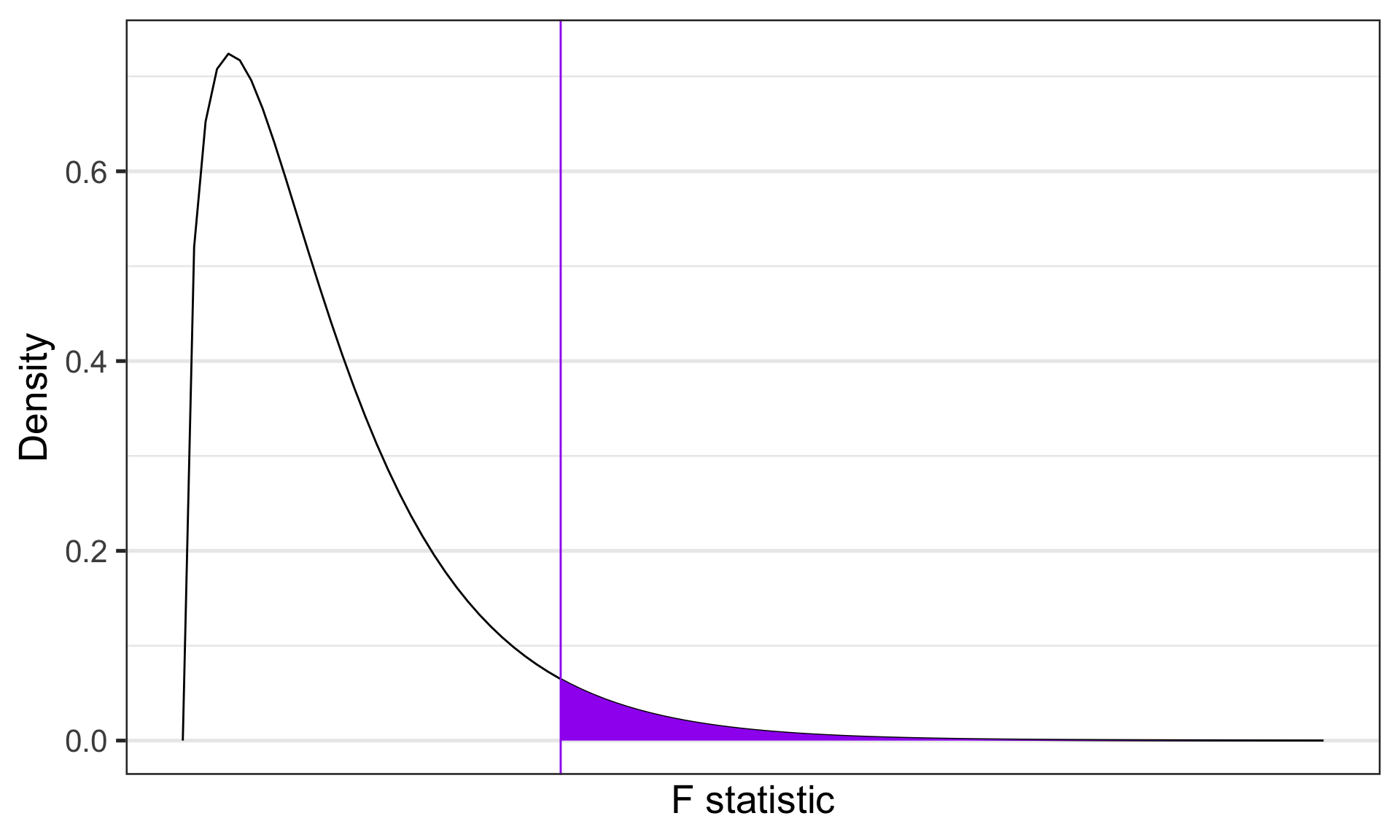
\(F\)-distributions are one-tailed tests. Recall that we’re interested in how far away our test statistic from the null \((F = 1).\)
Example
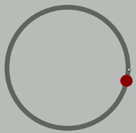
Participants performed an eye-hand coordination task while subjected to periodic 3-second bursts of 85 dB white noise played over earphones. The task required participants to keep a mouse pointer on a red dot that moved in a circular motion at a rate of 1 revolution per second. Participants performed the task until they allowed the pointer to stray from the rotating dot 10 times. The time (in seconds) at the 10th failure was recorded and is the outcome measure.
Example
The participants were randomly assigned to one of four noise Groups:
- controllable and predictable noise
- uncontrollable but predictable noise
- controllable but unpredictable noise
- uncontrollable and unpredictable noise.
When noise was predictable, the 3-second bursts of noise would occur regularly every 20 seconds.
When noise was unpredictable, the 3-second bursts would occur randomly (although every 20 seconds on average).
When noise was uncontrollable, participants could do nothing to prevent the noise from occurring.
When noise was controllable, participants were shown a button that would prevent the noise, but they were told, “the button is a safety measure, for your protection, but we would prefer that you not use it unless absolutely necessary.” No participants actually used the button.
Why is it important that the button was never used?
Why is random assignment important in this design?
  ID Predict Control Group Time Gender
1  1       0       1     3  504      F
2  2       0       0     1  443      F
3  3       1       1     4  292      M
4  4       0       1     3  398      F
5  5       1       1     4  119      F
6 6 0 0 1 545 F[1] "integer"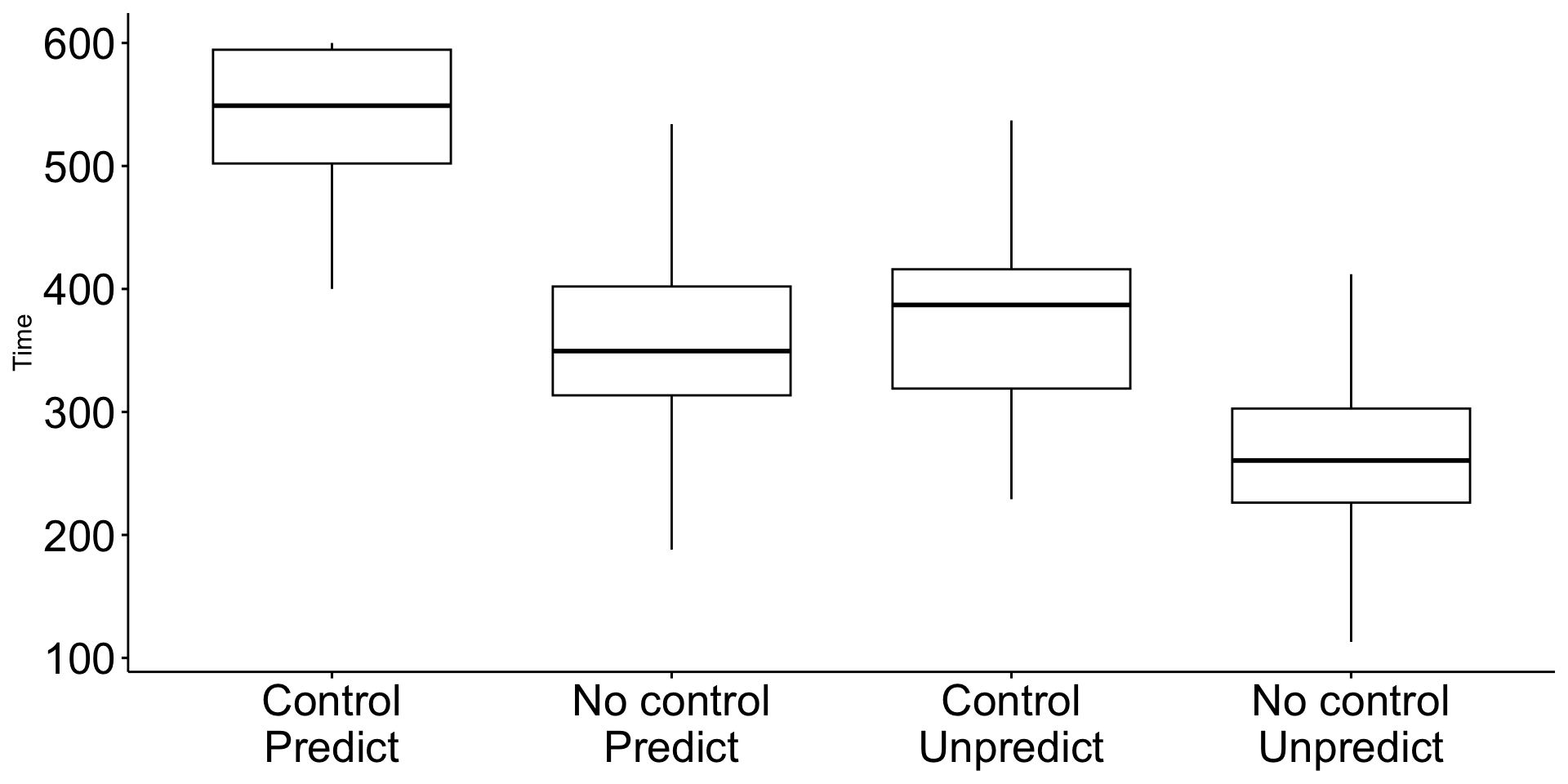
The pattern of means indicates that performance degrades with either uncontrollable noise or unpredictable noise. Noise that is both uncontrollable and unpredictable appears to be particularly disruptive.
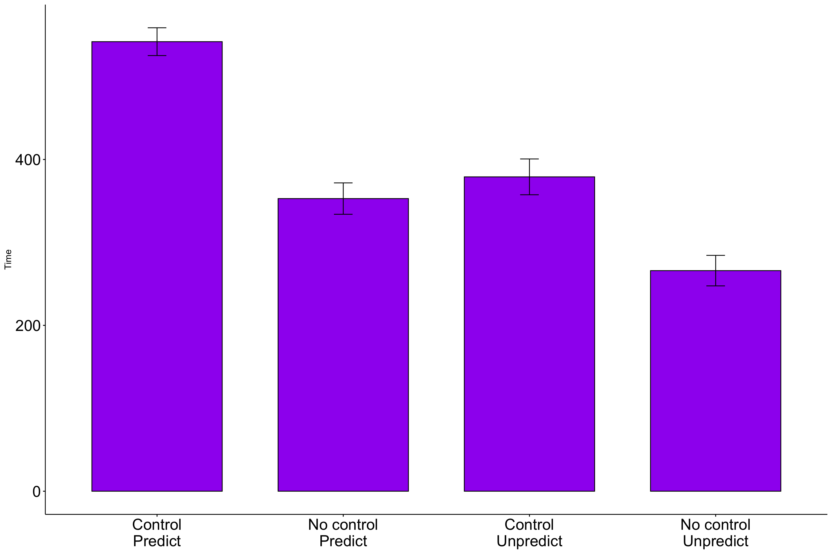
Addition of the confidence intervals indicates that the two extreme Groups are likely different from all of the other Groups.
Code
| Group_lab | N | Mean | SD |
|---|---|---|---|
| Control Predict | 47 | 542.04 | 57.11 |
| No control Predict | 52 | 352.85 | 67.98 |
| Control Unpredict | 45 | 379.04 | 71.85 |
| No control Unpredict | 56 | 265.98 | 68.68 |
The groups differ in their sample sizes, which can easily occur with free random assignment. There are advantages to equal sample sizes, so researchers often restrict random assignment to insure equal sample sizes across Groups.
Hard to tell if the variability in the four groups is homogeneous.
Run the ANOVA model
...
Analysis of Variance Table

Response: Time
           Df  Sum Sq Mean Sq F value                Pr(>F)
Group_lab   3 2000252  666751  149.82 < 0.00000000000000022 ***
Residuals 196  872288    4450
...
The \(F\) statistic is highly unusual in the \(F\) distribution, assuming the null hypothesis is true. We reject the null hypothesis.
Note: how does the output above compare to this output?
Analysis of Variance Table

Response: Time
           Df  Sum Sq Mean Sq F value                Pr(>F)
Group_lab   3 2000252  666751  149.82 < 0.00000000000000022 ***
Residuals 196  872288    4450
---
Signif. codes:  0 '***' 0.001 '**' 0.01 '*' 0.05 '.' 0.1 ' ' 1
We know the means are not equal, but the particular source of the inequality is not revealed by the \(F\) test.
One simple way to determine what is behind the significant \(F\) test is to compare each Group to all other Groups.
These comparisons take the general form of t-tests, but note some extensions:
- the pooled variance estimate comes from \(SS_{\text{residual}}\), meaning it pulls information from all groups
- the degrees of freedom for the t-test is \(N-k\), so using all data
Analysis of Variance Table

Response: Time
           Df  Sum Sq Mean Sq F value                Pr(>F)
Group_lab   3 2000252  666751  149.82 < 0.00000000000000022 ***
Residuals 196  872288    4450
---
Signif. codes:  0 '***' 0.001 '**' 0.01 '*' 0.05 '.' 0.1 ' ' 1
\(\hat{\sigma}_p = \sqrt{\frac{SS_{\text{residual}}}{N-k}} = \sqrt{\frac{872287.58}{200 - 4}} = 66.71\)
| Group_lab | N | Mean | SD |
|---|---|---|---|
| Control Predict | 47 | 542.04 | 57.11 |
| No control Predict | 52 | 352.85 | 67.98 |
| Control Unpredict | 45 | 379.04 | 71.85 |
| No control Unpredict | 56 | 265.98 | 68.68 |
To test the pairwise comparison, we use the old formulas for the independent samples t-test, except with this estimate of pooled sd and DF based on total N.
| Group_lab | N | Mean | SD |
|---|---|---|---|
| Control Predict | 47 | 542.04 | 57.11 |
| No control Predict | 52 | 352.85 | 67.98 |
\(\hat{\sigma}_p = \sqrt{\frac{SS_{\text{residual}}}{N-k}} = \sqrt{\frac{872287.58}{200 - 4}} = 66.71\)
\(\sigma_{D} = \hat{\sigma}_p\sqrt{\frac{1}{N_1} + \frac{1}{N_2}} = 66.71 \sqrt{\frac{1}{47} + \frac{1}{52}} = 13.43\)
\(t = \frac{M_1-M_2}{\sigma_D} = \frac{542.04 - 352.85 }{13.43} = 14.09\)
$emmeans
  Group_lab            emmean   SE  df lower.CL upper.CL
 Control\nPredict         542 9.73 196      523      561
 No control\nPredict      353 9.25 196      335      371
 Control\nUnpredict       379 9.94 196      359      399
 No control\nUnpredict    266 8.91 196      248      284

Confidence level used: 0.95

$contrasts
   contrast                                  estimate   SE  df t.ratio p.value
 Control\nPredict - No control\nPredict         189.2 13.4 196  14.091  <.0001
 Control\nPredict - Control\nUnpredict          163.0 13.9 196  11.715  <.0001
 Control\nPredict - No control\nUnpredict       276.1 13.2 196  20.918  <.0001
 No control\nPredict - Control\nUnpredict       -26.2 13.6 196  -1.929  0.0552
 No control\nPredict - No control\nUnpredict     86.9 12.8 196   6.761  <.0001
 Control\nUnpredict - No control\nUnpredict     113.1 13.4 196   8.466  <.0001
Family-wise error
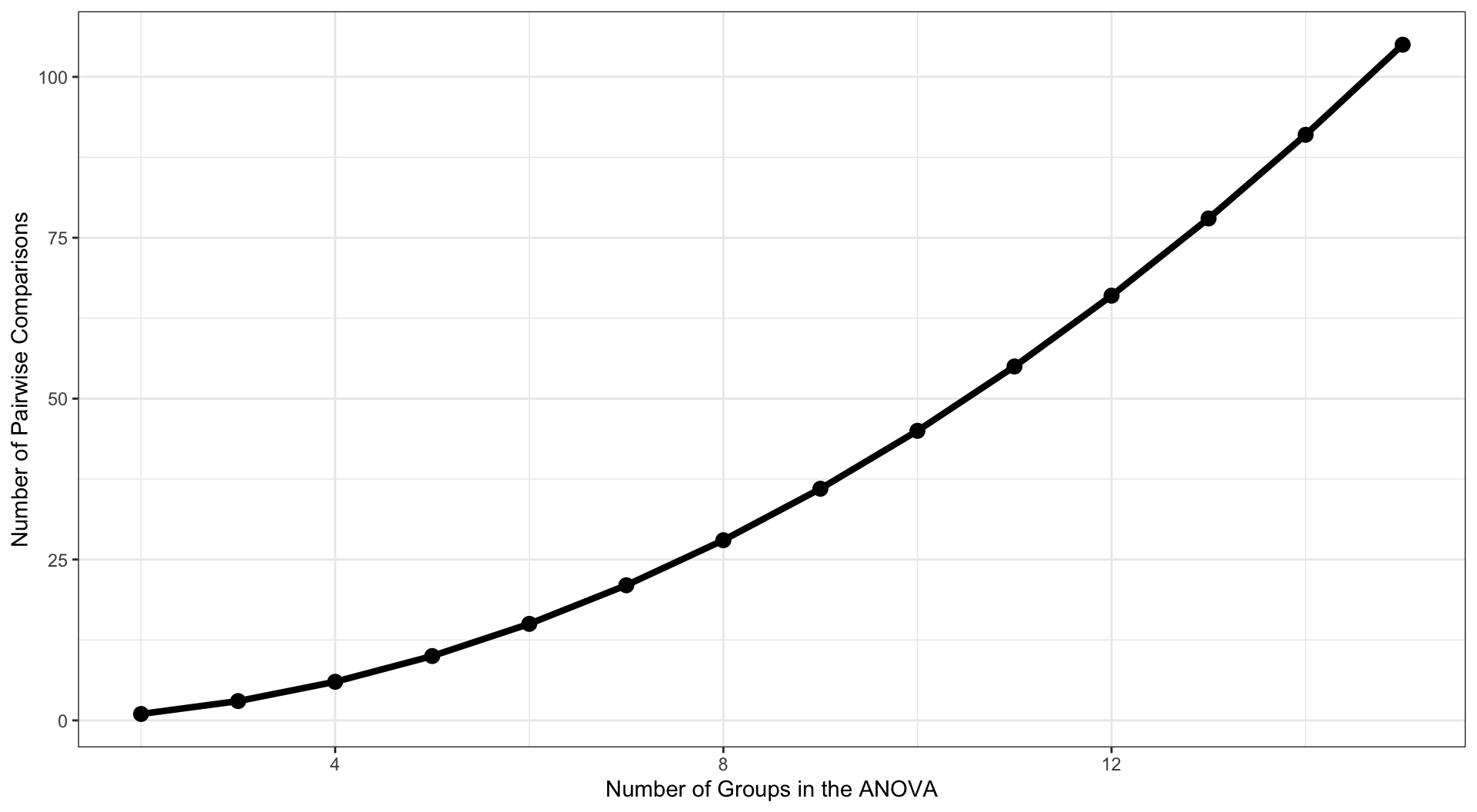
These pairwise comparisons can quickly grow in number as the number of Groups increases. With 4 (k) Groups, we have k(k-1)/2 = 6 possible pairwise comparisons.
As the number of groups in the ANOVA grows, the number of possible pairwise comparisons increases dramatically.
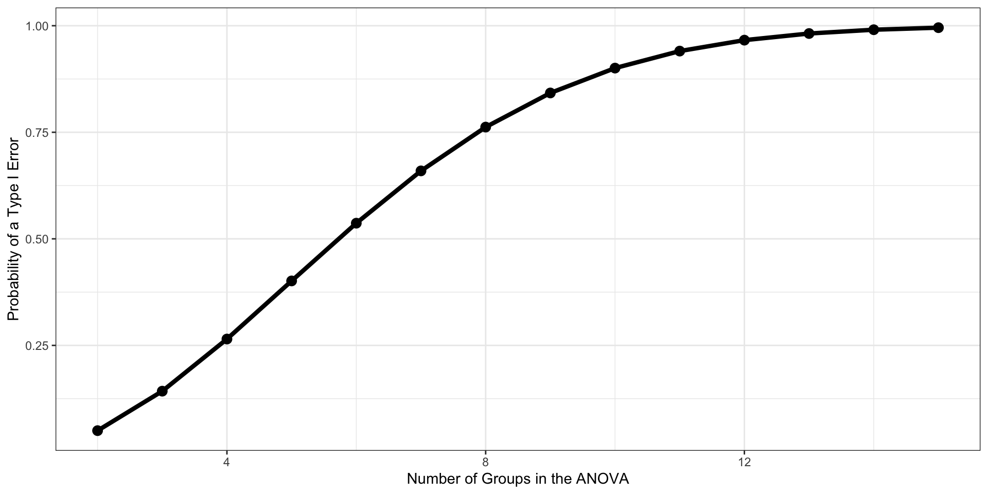
As the number of tests grows, and assuming the null hypothesis is true, the probability that we will make one or more Type I errors increases. To approximate the magnitude of the problem, we can assume that the multiple pairwise comparisons are independent. The probability that we don’t make a Type I error for one test is:
\[P(\text{No Type I}, 1 \text{ test}) = 1-\alpha\]
The probability that we don’t make a Type I error for two tests is:
\[P(\text{No Type I}, 2 \text{ test}) = (1-\alpha)(1-\alpha)\]
For C tests, the probability that we make no Type I errors is
\[P(\text{No Type I}, C \text{ tests}) = (1-\alpha)^C\]
We can then use the following to calculate the probability that we make one or more Type I errors in a collection of C independent tests.
\[P(\text{At least one Type I}, C \text{ tests}) = 1-(1-\alpha)^C\]
The Type I error inflation that accompanies multiple comparisons motivates the large number of “correction” procedures that have been developed.
Multiple comparisons, each tested with \(\alpha_{per-test}\), increases the family-wise \(\alpha\) level.
\[\large \alpha_{family-wise} = 1 - (1-\alpha_{per-test})^C\] Šidák showed that the family-wise a could be controlled to a desired level (e.g., .05) by changing the \(\alpha_{per-test}\) to:
\[\large \alpha_{per-wise} = 1 - (1-\alpha_{family-wise})^{\frac{1}{C}}\]
Bonferroni
Bonferroni (and Dunn, and others) suggested this simple approximation:
\[\large \alpha_{per-test} = \frac{\alpha_{family-wise}}{C}\]
This is typically called the Bonferroni correction and is very often used even though better alternatives are available.
$emmeans
  Group_lab            emmean   SE  df lower.CL upper.CL
 Control\nPredict         542 9.73 196      523      561
 No control\nPredict      353 9.25 196      335      371
 Control\nUnpredict       379 9.94 196      359      399
 No control\nUnpredict    266 8.91 196      248      284

Confidence level used: 0.95

$contrasts
   contrast                                  estimate   SE  df t.ratio p.value
 Control\nPredict - No control\nPredict         189.2 13.4 196  14.091  <.0001
 Control\nPredict - Control\nUnpredict          163.0 13.9 196  11.715  <.0001
 Control\nPredict - No control\nUnpredict       276.1 13.2 196  20.918  <.0001
 No control\nPredict - Control\nUnpredict       -26.2 13.6 196  -1.929  0.3312
 No control\nPredict - No control\nUnpredict     86.9 12.8 196   6.761  <.0001
 Control\nUnpredict - No control\nUnpredict     113.1 13.4 196   8.466  <.0001

P value adjustment: bonferroni method for 6 tests
The Bonferroni procedure is conservative. Other correction procedures have been developed that control family-wise Type I error at .05 but that are more powerful than the Bonferroni procedure. The most common one is the Holm procedure.
The Holm procedure does not make a constant adjustment to each per-test \(\alpha\). Instead it makes adjustments in stages depending on the relative size of each pairwise p-value.
Holm correction
- Rank order the p-values from largest to smallest.
- Start with the smallest p-value. Multiply it by its rank.
- Go to the next smallest p-value. Multiply it by its rank. If the result is larger than the adjusted p-value of next smallest rank, keep it. Otherwise replace with the previous step adjusted p-value.
- Repeat Step 3 for the remaining p-values.
- Judge significance of each new p-value against \(\alpha = .05\).
| Original p value | Rank | Rank x p | Holm | Bonferroni |
|---|---|---|---|---|
| 0.0012 | 6 | 0.0072 | 0.0072 | 0.0072 |
| 0.0023 | 5 | 0.0115 | 0.0115 | 0.0138 |
| 0.0450 | 4 | 0.1800 | 0.1800 | 0.2700 |
| 0.0470 | 3 | 0.1410 | 0.1800 | 0.2820 |
| 0.0530 | 2 | 0.1060 | 0.1800 | 0.3180 |
| 0.2100 | 1 | 0.2100 | 0.2100 | 1.0000 |
$emmeans
  Group_lab            emmean   SE  df lower.CL upper.CL
 Control\nPredict         542 9.73 196      523      561
 No control\nPredict      353 9.25 196      335      371
 Control\nUnpredict       379 9.94 196      359      399
 No control\nUnpredict    266 8.91 196      248      284

Confidence level used: 0.95

$contrasts
   contrast                                  estimate   SE  df t.ratio p.value
 Control\nPredict - No control\nPredict         189.2 13.4 196  14.091  <.0001
 Control\nPredict - Control\nUnpredict          163.0 13.9 196  11.715  <.0001
 Control\nPredict - No control\nUnpredict       276.1 13.2 196  20.918  <.0001
 No control\nPredict - Control\nUnpredict       -26.2 13.6 196  -1.929  0.0552
 No control\nPredict - No control\nUnpredict     86.9 12.8 196   6.761  <.0001
 Control\nUnpredict - No control\nUnpredict     113.1 13.4 196   8.466  <.0001

P value adjustment: holm method for 6 tests
ANOVA is regression
We saw in the previous lecture that we can accommodate categorical variables into a regression model. How does this compare to ANOVA?
- Same omnibus test of the model!
*(Really the same model, but packaged differently.)
- When would you use one versus the other?
ANOVA
More traditional for 3+ groups
Comparing/controlling multiple categorical variables
Regression
Best for two groups
Incorporating continuous predictors too
Good for 3+ groups when you have more specific hypotheses (contrasts)
One benefit to using the ANOVA framework instead of the regression framework is that you can estimate the total variability captured by one categorical variable controlling for another categorical or continuous variable with ease.
\(\eta^2\) (eta-squared) is a standardized measure of effect size used in analyses of variance. This effect size is the proportion of variance in Y that is accounted for by one independent variable.
\[\eta^2 = \frac{SS_{variable}}{SS_{total}}\]
For example, what if we believed gender was associated with performance on the noise burst task.
Analysis of Variance Table

Response: Time
           Df  Sum Sq Mean Sq F value                Pr(>F)
Group_lab   3 2000252  666751 160.853 < 0.00000000000000022 ***
Gender      1   63993   63993  15.438             0.0001183 ***
Residuals 195  808294    4145
---
Signif. codes: 0 '***' 0.001 '**' 0.01 '*' 0.05 '.' 0.1 ' ' 1 eta.sq eta.sq.part
Group_lab 0.62526817 0.6896430
Gender 0.02227757 0.0733625Contrasts
Recall from the previous lecture that dummy codes are series of 1’s and 0’s with one group established as the reference group.
contrasts(rotate$Group_lab) = contr.treatment(n = 4, base = 3)
summary(lm(Time ~ Group_lab, data = rotate))
...
Coefficients:
Estimate Std. Error t value Pr(>|t|)
(Intercept) 379.044 9.945 38.115 < 0.0000000000000002 ***
Group_lab1 162.998 13.914 11.715 < 0.0000000000000002 ***
Group_lab2 -26.198 13.583 -1.929 0.0552 .
Group_lab4 -113.062 13.356 -8.466 0.00000000000000592 ***
...Contrasts
But there’s more you can do!
You’re not restricted to simple dummy coding. Choosing another variant of contrast codes allows you to test more specific hypotheses. There are some common coding schemes.
For example, deviation coding (sometimes called “effect coding”):
...
Coefficients:
            Estimate Std. Error t value             Pr(>|t|)
(Intercept)  384.979      4.734  81.314 < 0.0000000000000002 ***
Group_lab1   157.064      8.352  18.805 < 0.0000000000000002 ***
Group_lab2   -32.133      8.075  -3.979            0.0000973 ***
Group_lab3    -5.934      8.477  -0.700                0.485
...
Contrasts
You can create a contrast matrix that tests any number of hypotheses, like whether groups 1 and 3 are different from group 4. The rules for setting up contrast codes are:
The sum of the weights across all groups for each code variable must equal 0. (Sum down the column = 0).
The sum of the product of each pair of code variables, \(C_1C_2,\) must equal 0. (This is challenging when your groups are unequal sizes).
The difference between the value of the set of positive weights and the set of negative weights should equal 1 for each code variable (column).
contrasts(rotate$Group_lab) = contr.treatment(4)
library(multcomp)
Lmatrix = matrix(
  c( 0,   1,   -1,    0,  # G2 vs G3
    1/2, 1/2,   0,   -1,  # G1/G2 vs G4
    1/2, 1/2, -1/2, -1/2, # G1/G2 vs G3/G4
    1/3, 1/3,  1/3,  -1), # G1/G2/G3 vs G4
  ncol = 4, byrow = T)
mod = lm(Time ~ Group_lab, data = rotate)
summary(glht(mod,
             linfct = mcp(Group_lab = Lmatrix)))
     Simultaneous Tests for General Linear Hypotheses

Multiple Comparisons of Means: User-defined Contrasts


Fit: lm(formula = Time ~ Group_lab, data = rotate)

Linear Hypotheses:
       Estimate Std. Error t value Pr(>|t|)
1 == 0  -26.198     13.583  -1.929    0.137
2 == 0  181.462     11.160  16.260   <0.001 ***
3 == 0  124.931      9.469  13.194   <0.001 ***
4 == 0  158.662     10.512  15.094   <0.001 ***
---
Signif. codes:  0 '***' 0.001 '**' 0.01 '*' 0.05 '.' 0.1 ' ' 1
(Adjusted p values reported -- single-step method)
Next time…
Assumptions and diagnostics