Lecture 14 will be pre-recorded by end of day tomorrow
Homework #2 due Monday
Time to find data for your final project
3 continuous variables
1 categorical variable
library(ggdag)library(tidyverse)
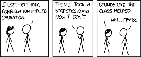
Correlation does not imply
causation
always?
It’s true that presence of a correlation is not sufficient to demonstrate causality. However, this axiom has been overgeneralized to the point where psychologists refuse to acknowledge any observational work as indicative of causal models. This ignores a rich history of modeling work that demonstrated that – under certain assumptions – correlational work can uncover the real causal mechanisms.
Moreover, the causal modeling tradition informs even analyses which are not necessarily interested in proving causation.
Karl Pearson (1857-1936)
Francis Galton demonstrates that one phenomenon – regression to the mean – is not caused by external factors, but merely the result of natural chance variation.
Pearson (his student) takes this to the extreme, which is causation can never be proven.
“Force as a cause of motion is exactly on the same footing as a tree-god as a cause of growth.” (Pearson, 1892, pp 119)
Sewall Wright (1889-1988)
Geneticist; studied guinea pigs at the USDA; then teaches zoology at the University of Chicago, then University of Wisconsin-Madison
Developed path models as a way to identify causal forces and estimate values
Rebuke from mathematical community, including from Ronald Fisher (who also disagreed with Wright’s theories of evolution)
Extensively studied this history of causation in statistics, inferring causality through data, and the development of path analysis
Popularized the use of causal graph theory
Article: Rohrer (2018)
Thinking clearly about correlation and causation
Psychologists are interested in inherently causal relationships.
e.g., how does social class cause behavior?
According to Rohrer, how have psychologists attempted to study causal relationships while avoiding issues of ethicality and feasibility?
It is impossible to infer causation from correlation without background knowledge about the domain.
Experimental studies require assumptions as well.
The work by these figures (Pearson*, Wright, Pearl, Rohrer) and others can be used to understand the role of covariates in regression models.
Regression models imply causality. Pretending that they don’t is silly and potentially dangerous.
Why include covariates or controls (e.g., age, gender) in a regression model?
Remove third-variable problem
Isolate unique contribution of IV(s) of interest
Reduce non-random noise in DV
Each covariate needs to be justified theoretically! How can we do this?
Directed Acyclic Graphics (DAGs)
Visual representations of causal assumptions
DAG models are qualitative descriptions of your theory. This tool is used before data collection and analysis to plan the most appropriate regression model.
You will not use a DAG model to estimate numeric values.
Directed Acyclic Graphics (DAGs)
The benefit of DAG models is that they
help you clarify the causal model at the heart of your research question, and
identify which variables you should and should not include in a regression model, based on your causal assumptions.
Paths lead from one node to the next; they can include multiple nodes, and there may be multiple paths connecting two nodes. There are three kinds of paths:
Chains
Forks
Inverted forks
Paths: Chains (Mediation)
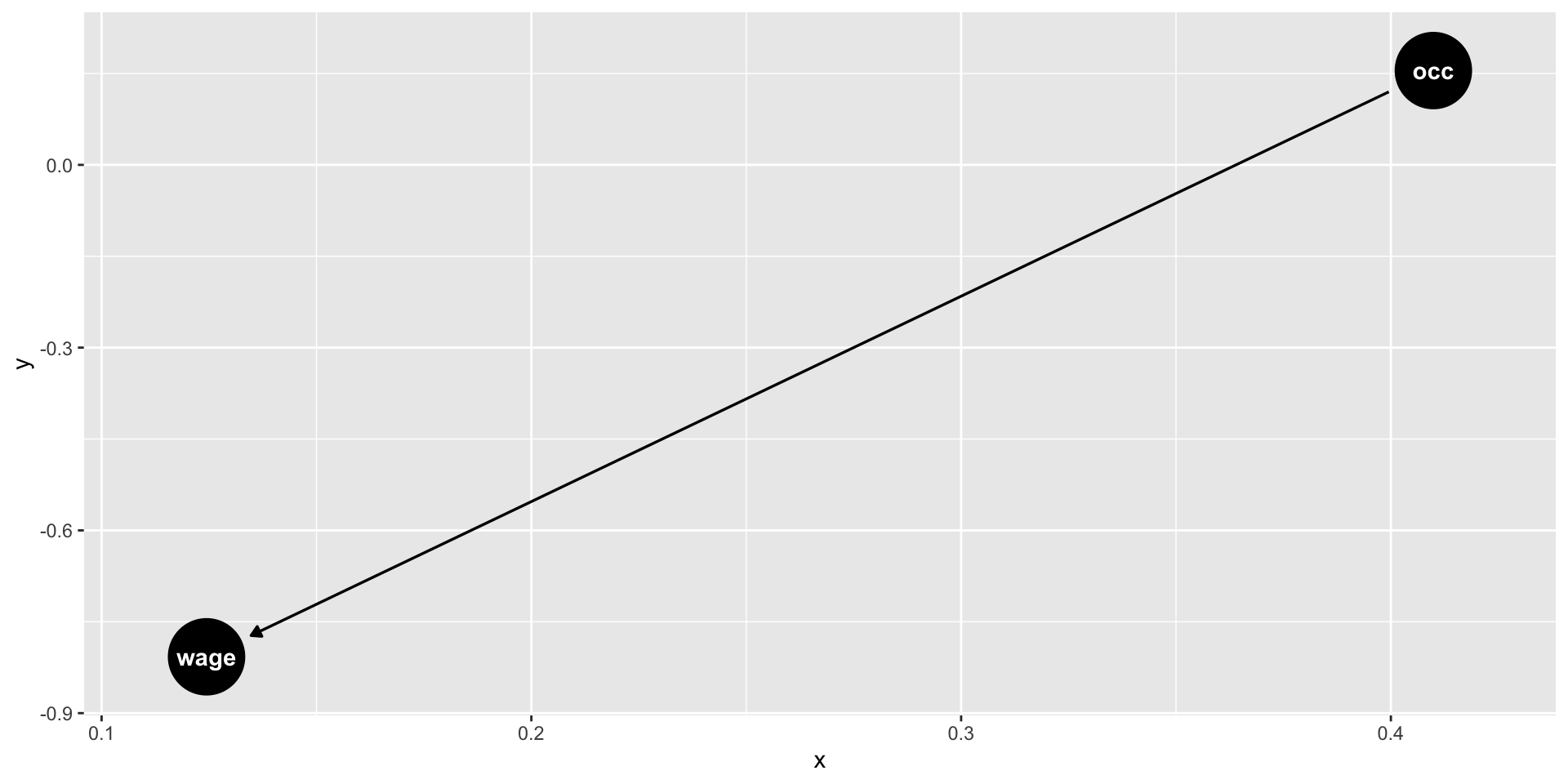
Chains have the structure
A → B → C.
Chains can transmit associations from the node at the beginning to the node at the end, meaning that you will find a correlation between A and C. These associations represent real causal relationships.
DAG models are most useful for psychological scientists thinking about which variables to include in a regression model. Recall that one of the uses of regression is to statistically control for variables when estimating the relationship between an X and Y in our research question. Which variables should we be statistically controlling for?
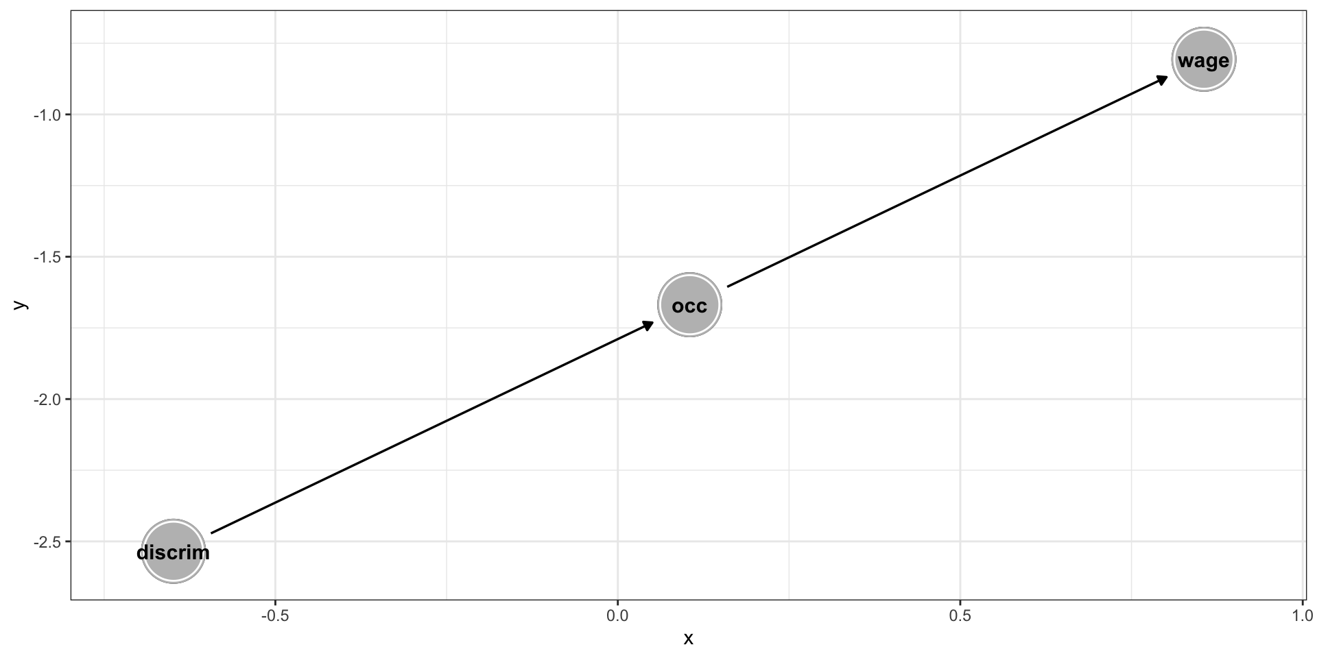
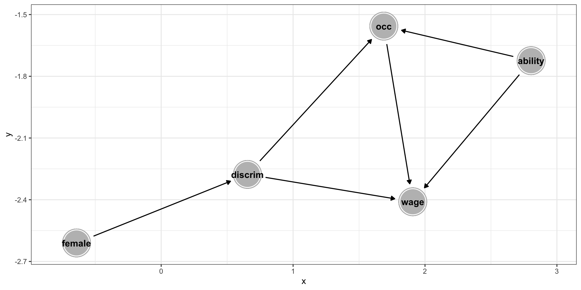
Confounding
We can see with DAG models that we should be controlling for constructs create forks, or a construct that causes both our X and Y variable. These constructs are known as confounds, or constructs that represent common causes of our variables of interest.
We may also want to control for variables that cause Y but are unrelated to X, as this can increase power by reducing unexplained variance in Y (think about SS).
Importantly, we probably do not want for variables that causes just X and not Y.
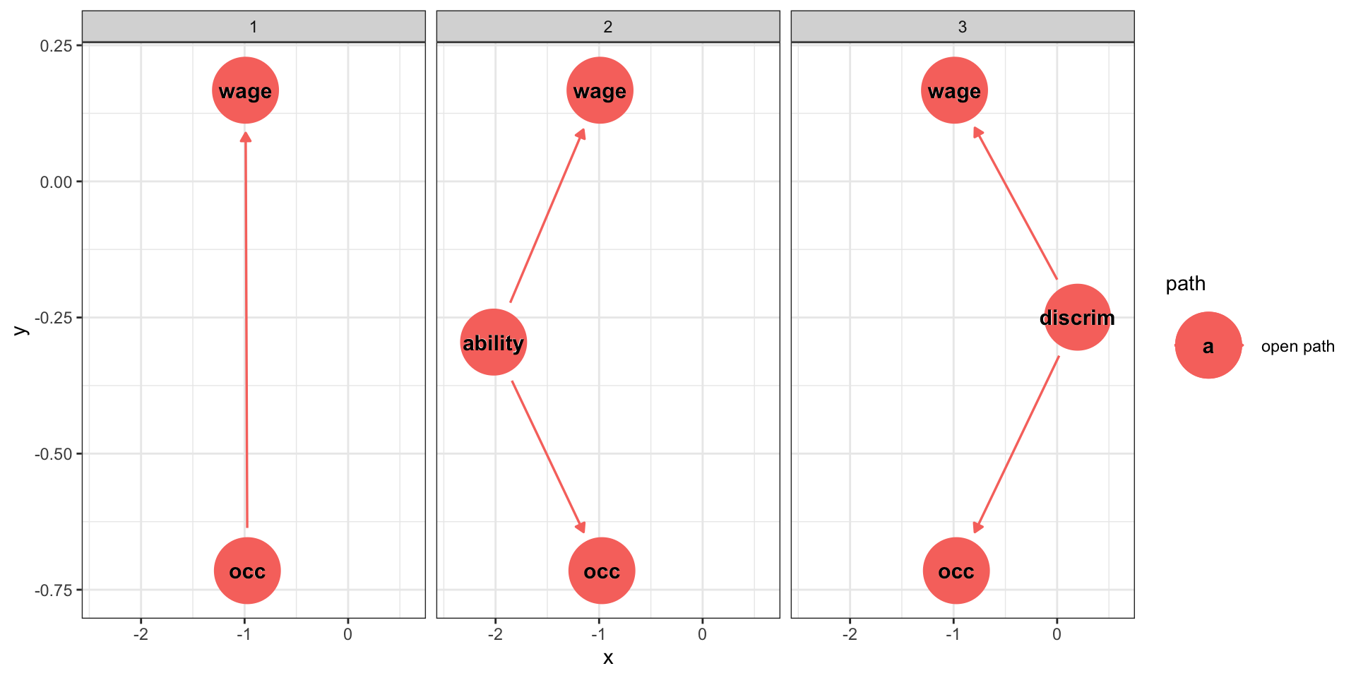
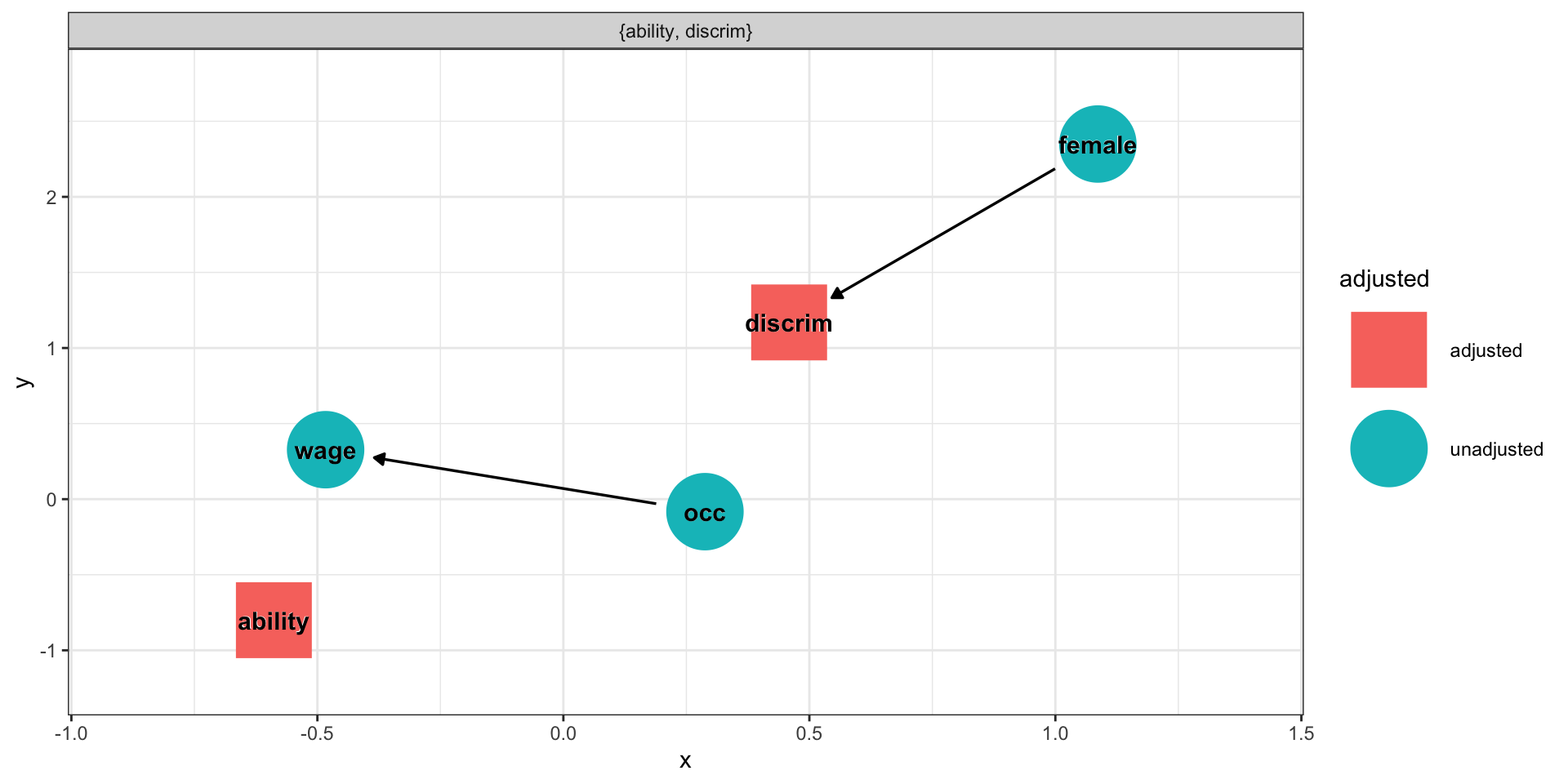
Confounds open “back-doors” between variables that act like causal pathways, but are not. But closing off the back doors, we isolate the true causal pathways, if there are any, and our regression models will estimate those.
Based on the causal structure I hypothesized last slide, if I want to estimate how much occupation causes income, I should control for discrimination and ability, but I don’t need to control for gender.
We can see with forks that controlling for confounds improves our ability to correctly estimate causal relationships. So controlling for things is good…
Except the other thing that DAGs should teach us is that controlling for the wrong things can dramatically hurt our ability to estimate true causal relationships and can create spurious correlations, or open up new associations that don’t represent true causal pathways.
Let’s return to the other two types of paths, chains and inverted forks.
Control in chains
Chains represent mediation; the effect of construct A on C is through construct B.
Controlling for mediators removes the association of interest from the model – you may be removing the variance you most want to study!
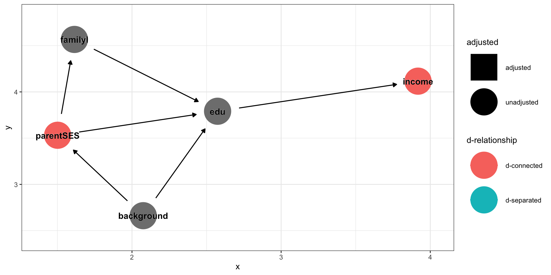
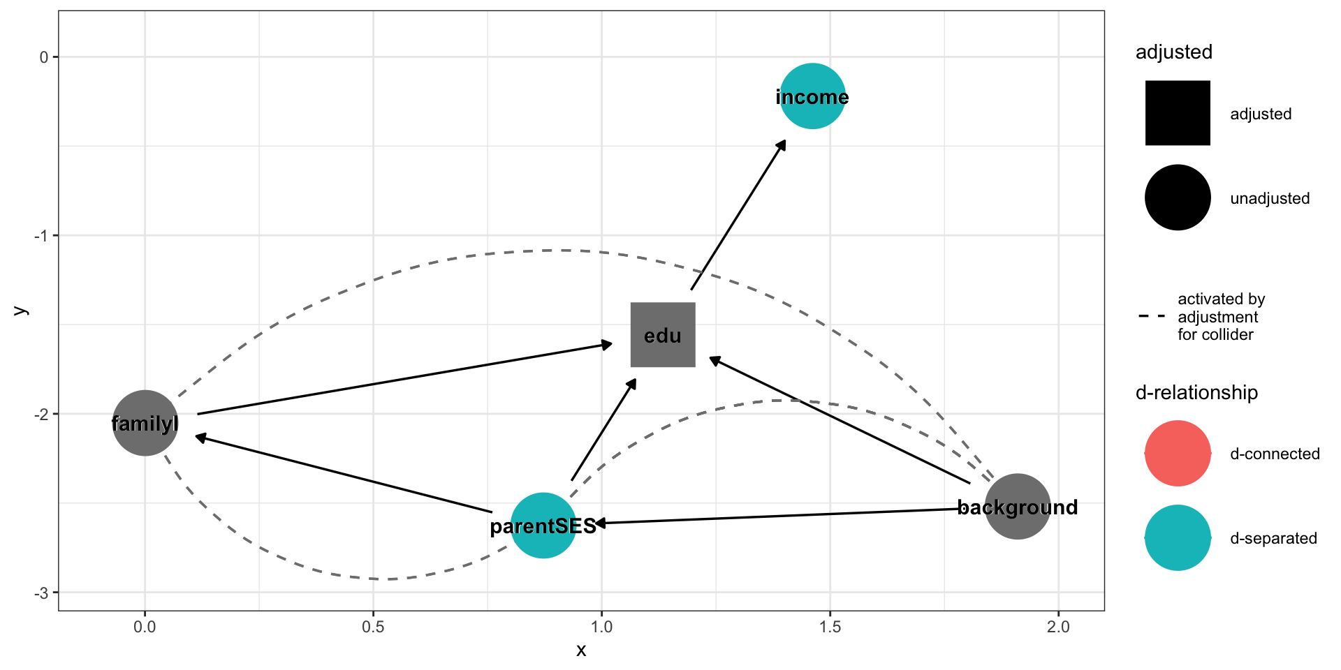
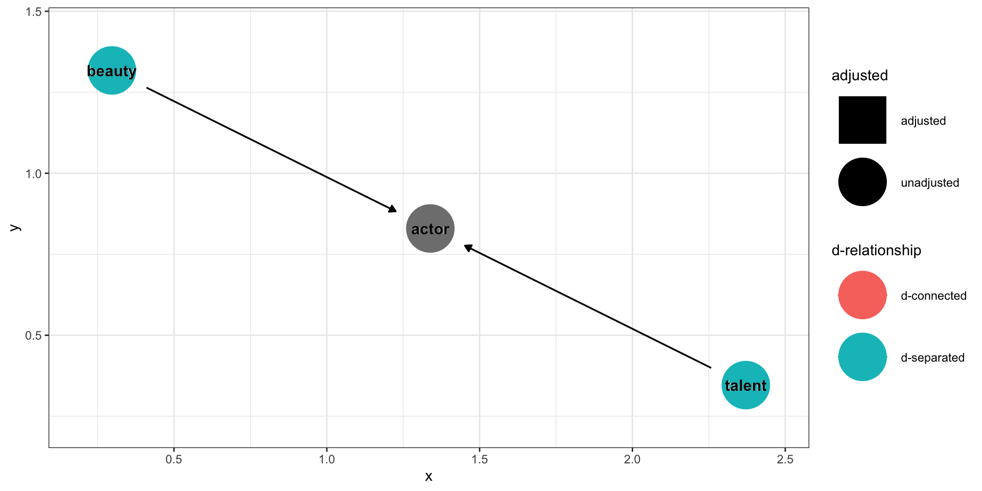
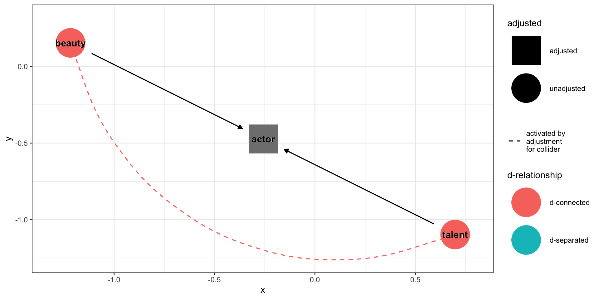
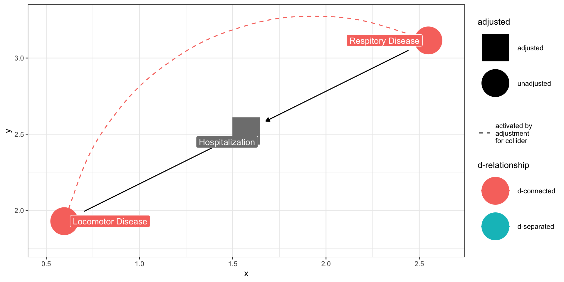
Inverted forks also teach us what not to control for: colliders. A collider for a pair of constructs is any third construct that is caused by both constructs in the pair. Controlling for (or conditioning on) these variables introduces bias into your estimates.
Sampling from a specific environment (or a specific subpopulation) can result in collider bias.
Be wary of:
Missing data
Subgroup analysis
Any post treatment variables
ggdag_dseparated(dag.obj, controlling_for ="c", text =FALSE, use_labels ="label") +theme_bw()
Any variables in a model, including moderators, act as colliders.
Example
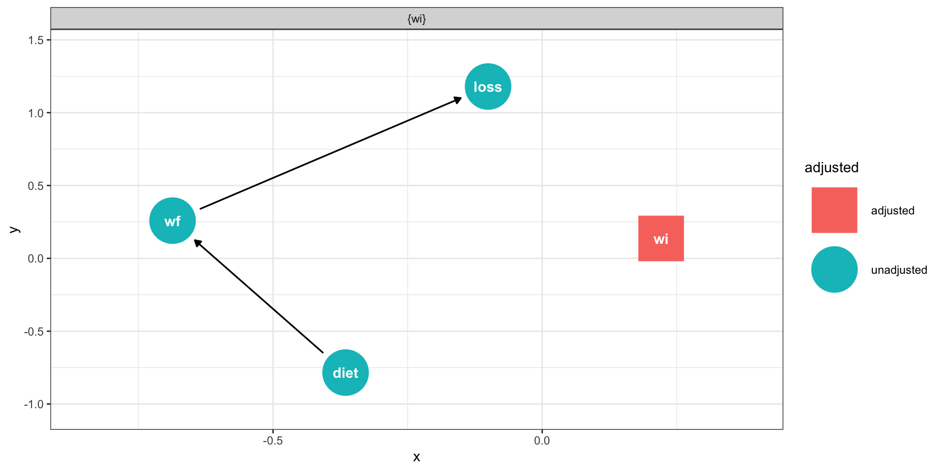
A health researcher is interested in studying the relationship between dieting and weight loss. She collects a sample of participants, measures their weight, and then asks whether they are on a diet. She returns to these participants two months later and measures their final weight and how much weight they lost. What should the researcher control when assessing the relationship between dieting and weight loss?
dag.obj =dagify(diet ~ wi, wf ~ diet + wi, loss ~ wi + wf,exposure ="diet", outcome ="loss")
ggdag_adjustment_set(dag.obj) +theme_bw()
The researcher should control for the initial weight (fork/third variable), but not the final weight (chain/mediator).
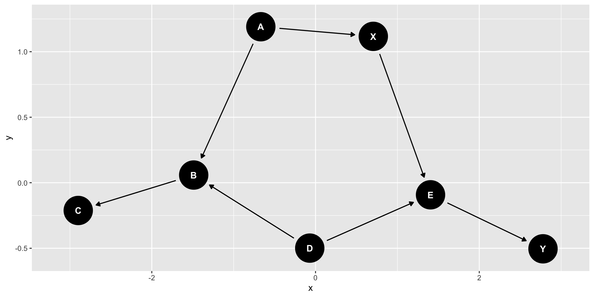
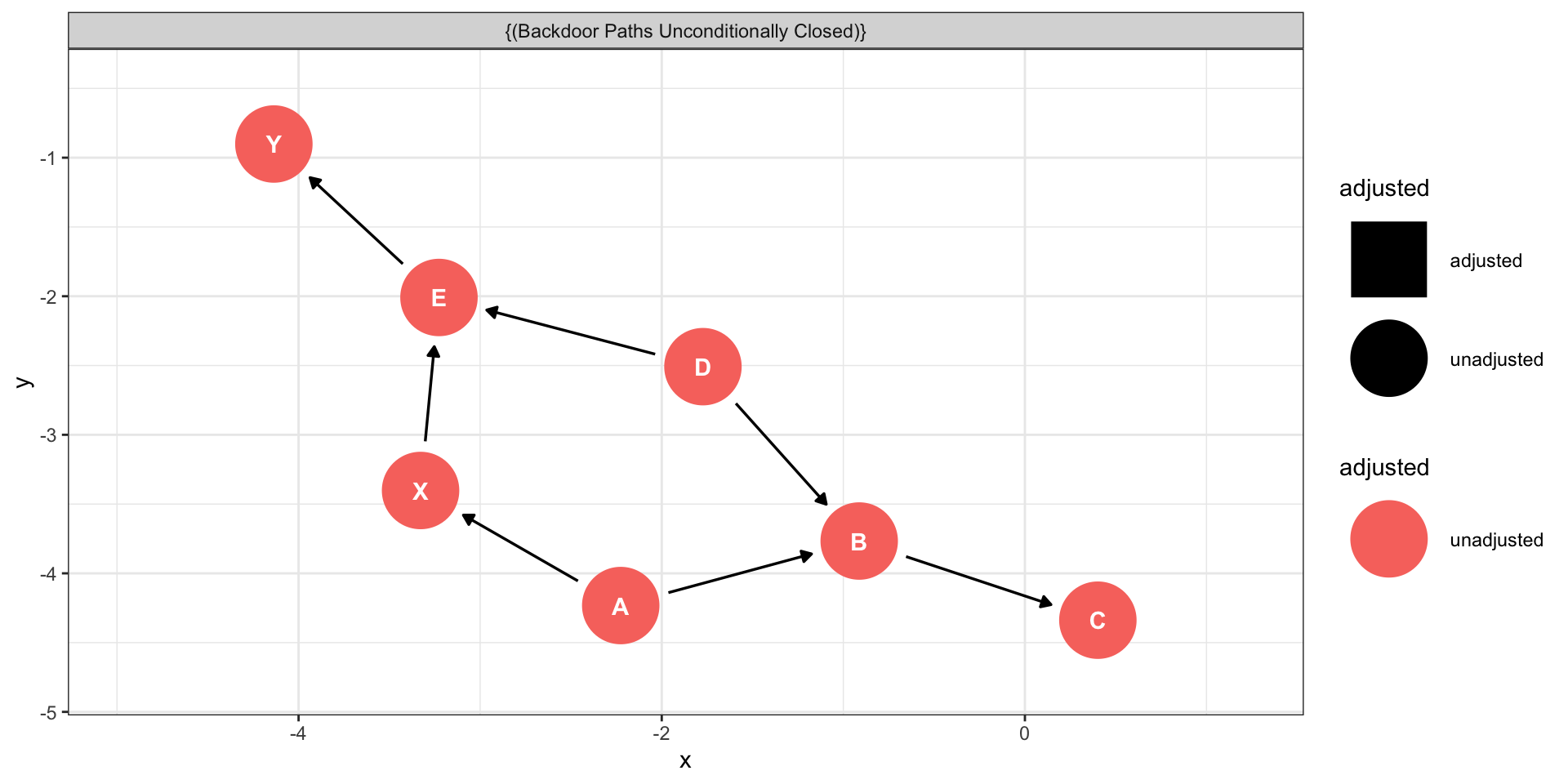
The researcher is studying the association between X and Y. What should be controlled?
ggdag_adjustment_set(dag.obj) +theme_bw()
There is a strong assumption of DAG models, and that it’s that no relevant variables have been omitted from the graph and that causal pathways have been correctly specified. This is a tall order, and potentially impossible to meet. Moreover, two different researchers may reasonably disagree with what the true model looks like.
It’s your responsibility to decide for yourself what you think the model is, provide as much evidence as you can, and listen when an open mind to those who disagree.