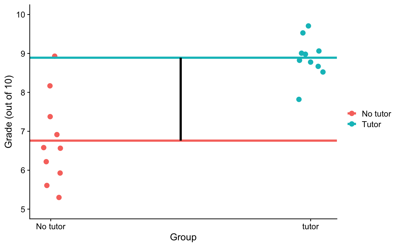
\(b_1\) is the difference in means between the two groups if the two groups have the same average level of hours studying or holding study constant.
This, by the way, is ANCOVA.
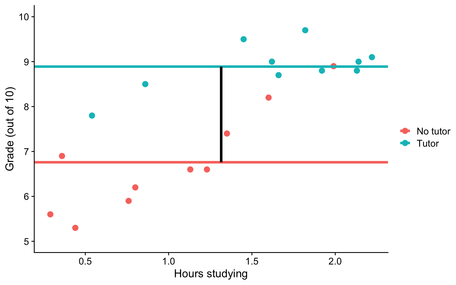
Visualizing
Code
mod =lm(grade ~ study + tutor_lab, data = t_data)t_data$pmod =predict(mod)predict.2=data.frame(study =rep(mean(t_data$study), 2), tutor_lab =c("No tutor", "Tutor"))predict.2$grade =predict(mod, newdata = predict.2) predict.2=cbind(predict.2[1,], predict.2[2,])names(predict.2) =c("x1", "d1", "y1", "x2", "d2", "y2")ggplot(t_data, aes(study,grade, color = tutor_lab)) +geom_point(size =3, aes(color = tutor_lab)) +geom_smooth(aes(y = pmod), method ="lm", se = F)+geom_segment(aes(x = x1, y = y1, xend = x2, yend = y2), data = predict.2, inherit.aes = F, size =1.5)+labs(x ="Hours studying", y ="Grade (out of 10)", color ="") +scale_y_continuous(limits =c(5,10)) + cowplot::theme_cowplot()
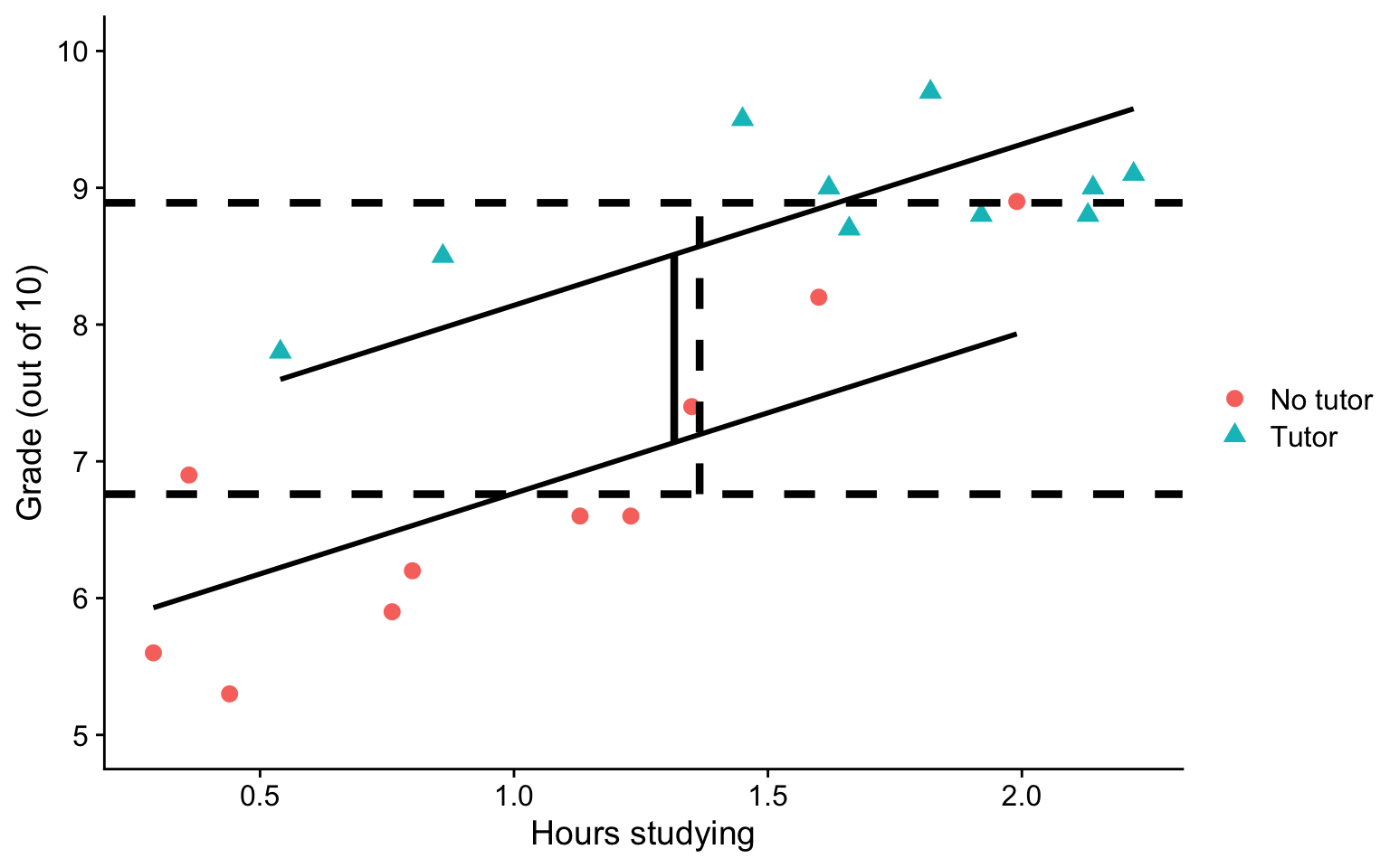
Visualizing
Code
ggplot(t_data, aes(study, grade, group = tutor_lab)) +geom_point(size =3, aes(shape = tutor_lab, color = tutor_lab)) +geom_smooth(aes(y = pmod), method ="lm", se = F, color ="black")+geom_hline(aes(yintercept = M), linetype ="dashed",data = means, size =1.5) +geom_segment(aes(x = x1, y = y1, xend = x2, yend = y2), data = predict.2, inherit.aes = F, size =1.5) +geom_segment(aes(x = x1+.05, y = y1, xend = x2+.05, yend = y2), data = predict.1, inherit.aes = F, size =1.5, linetype ="dashed") +labs(x ="Hours studying", y ="Grade (out of 10)", color ="", shape ="") +scale_y_continuous(limits =c(5,10)) + cowplot::theme_cowplot()
What are interactions?
When we have two variables, A and B, in a regression model, we are testing whether these variables have additive effects on our outcome, Y. That is, the effect of A on Y is constant over all values of B.
Example: Studying and working with a tutor have additive effects on grades; no matter how many hours I spend studying, working with a tutor will improve my grade by 2 points.
What are interactions?
However, we may hypothesis that two variables have joint effects, or interact with each other. In this case, the effect of A on Y changes as a function of B.
Example: Working with a tutor has a positive impact on grades but only for individuals who do not spend a lot of time studying; for individuals who study a lot, tutoring will have little or no impact.
This is also referred to as moderation.
Interactions (moderation) tell us whether the effect of one IV (on a DV) depends on another IV.
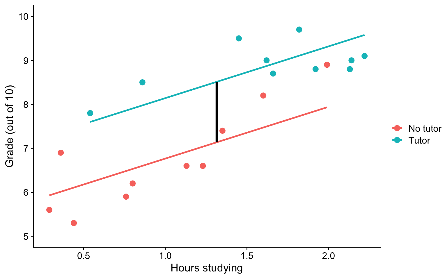
Interactions
Now extend this example to include joint effects, not just additive effects:
ggplot(t_data, aes(study, grade, color = tutor_lab)) +geom_point(size =3) +geom_smooth(method ="lm", se = F)+labs(x ="Hours studying", y ="Grade (out of 10)", color ="") + cowplot::theme_cowplot()
Where should we draw the segment to compare means?
the linear effect of the product of hours studying and tutoring
the degree of curvature in the regression plane
how much the slope of study differs for the two tutoring groups
how much the effect of tutoring changes for for every one 1 hour increase in studying.
Terms
Interactions tell us whether the effect of one IV (on a DV) depends on another IV. In this case, the effect of tutoring depends on a student’s time spent studying. Tutoring has a large effect when a student’s spends little time studying, but a small effect when the amount of time studying is high.
\(b_3\) is referred to as a “higher-order term.”
Higher-order terms are those terms that represent interactions.
Terms
Lower-order terms change depending on the values of the higher-order terms. The value of \(b_1\) and \(b_2\) will change depending on the value of \(b_3\).
These values represent “conditional effects” (because the value is conditional on the level of the other variable). In many cases, the value and significance test with these terms is either meaningless (if an IV is never equal to 0) or unhelpful, as these values and significance change across the data.
Conditional effects and simple slopes
The regression line estimated in this model is quite difficult to interpret on its own. A good strategy is to decompose the regression equation into simple slopes, which are determined by calculating the conditional effects at a specific level of the moderating variable.
Simple slope: the equation for Y on X at different levels of Z
Conditional effect: the slope coefficients in the full regression model that can change. These are the lower-order terms associated with a variable. E.g., studying has a conditional effect on grade.
The conditional nature of these effects is easiest to see by “plugging in” different values for one of your variables. Return to the regression equation estimated in our tutoring data:
Often we graph the simple slopes as a way to understand the interaction. The shape of the lines in the graph are informative and help us interpret conceptually what’s happening.
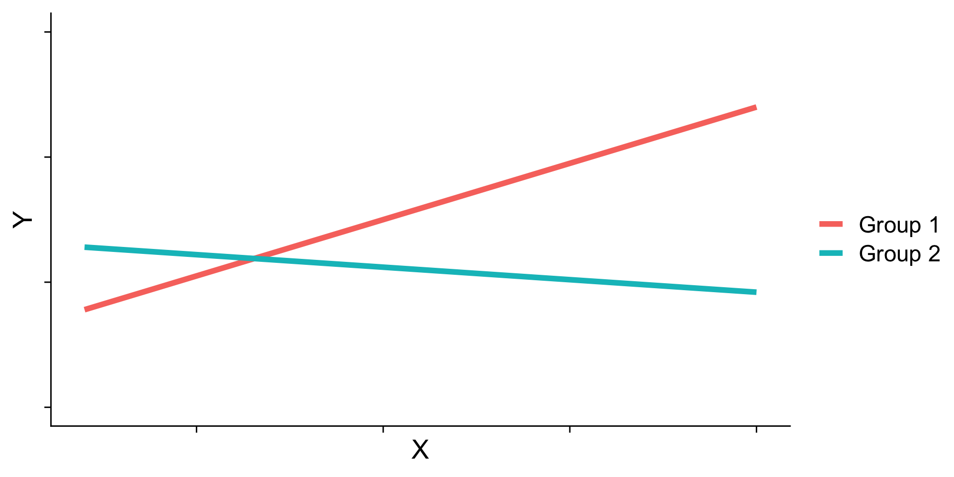
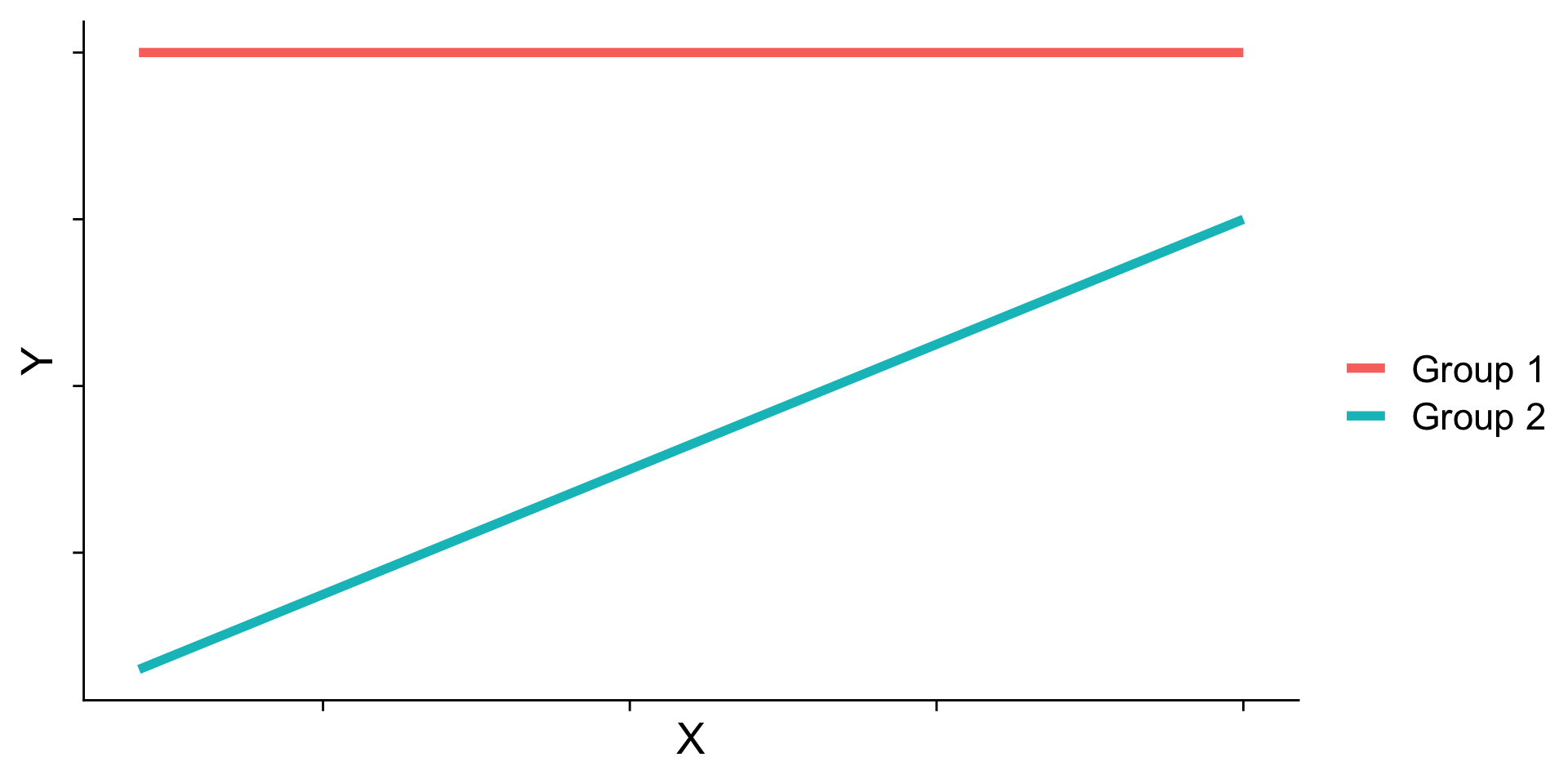
Cross-over interactions
Ordinal interactions
Interaction shapes
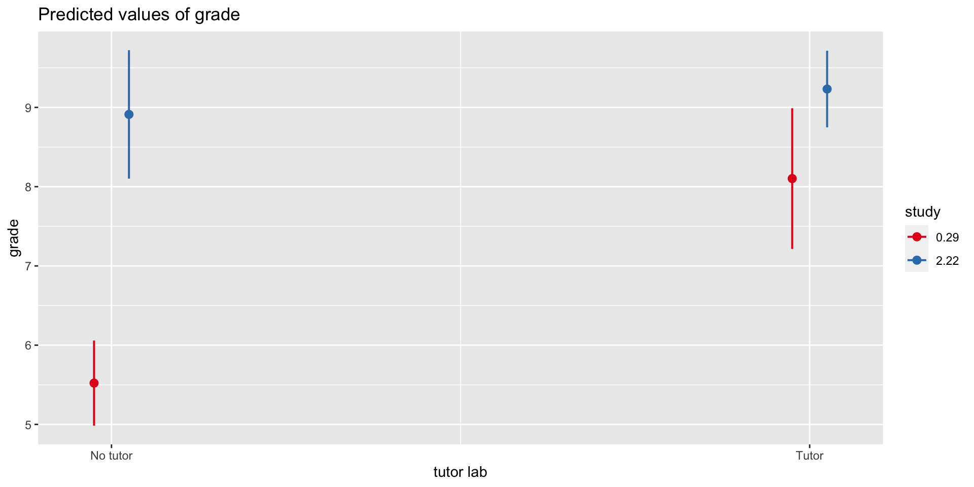
Ordinal interactions (beware…)
library(sjPlot)plot_model(mod3, type ="int")
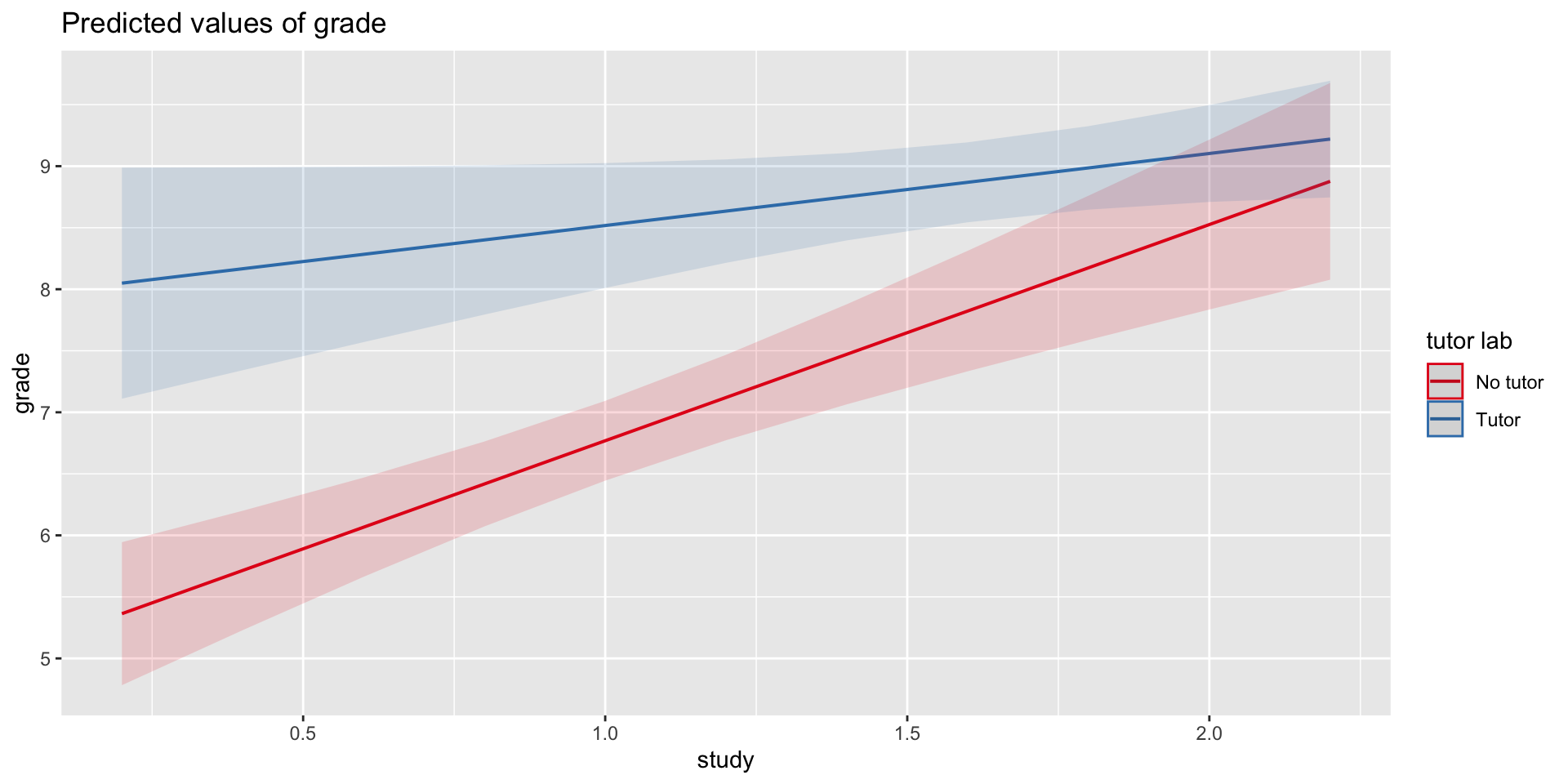
library(sjPlot)plot_model(mod3, type ="pred", terms =c("study", "tutor_lab"))
Simple slopes - Significance tests
The slope of studying at a specific level of tutoring (1 or 0) is a combination of both \(b_1\) and \(b_3\):
\[\large se_{b@D} = \sqrt{se_{b_1}^2 + (2 * D * cov_{b_1b_3})+ (D^2 se_{b_3}^2)}\] In this formula, \(cov_{b_1b_3}\) refers to the covariance of the coefficients, not the covariance of the variables. This may seem a strange concept, as we only ever have one value for \(b_1\) and \(b_3\) – the covariance of these coefficients refer to idea that if we randomly sample from a population, estimate the coefficients each time, and then examine the covariance of coefficients across random samples, it will not be 0.
Next, we can use the contrast function to look at pairwise comparisons of these fitted values.
combins =emmeans(mod3, ~ study*tutor_lab, at=mylist)contrast(combins, "pairwise", by ="study")
study = 0.5:
 contrast         estimate    SE df t.ratio p.value
 No tutor - Tutor   -2.335 0.452 16  -5.160  0.0001

study = 1.0:
 contrast         estimate    SE df t.ratio p.value
 No tutor - Tutor   -1.749 0.307 16  -5.693  <.0001

study = 2.0:
 contrast         estimate    SE df t.ratio p.value
 No tutor - Tutor   -0.578 0.406 16  -1.424  0.1736
Centering
The regression equation built using the raw data is not only diffiuclt to interpret, but often the terms displayed are not relevant to the hypotheses we’re interested.
\(b_0\) is the expected value when all predictors are 0, but this may never happen in real life
\(b_1\) is the effect of tutoring when hours spent studying is equal to 0, but this may not ever happen either.
Centering your variables by subtracting the mean from all values can improve the interpretation of your results.
Remember, a linear transformation does not change associations (correlations) between variables. In this case, it only changes the interpretation for some coefficients.
t_data = t_data %>%mutate(study_c = study -mean(study))head(t_data)
mod4 =lm(grade ~ study*tutor, data = t_data2)summary(mod4)
Call:
lm(formula = grade ~ study * tutor, data = t_data2)

Residuals:
     Min       1Q   Median       3Q      Max
-0.85839 -0.04148 -0.01957  0.03061  0.91044

Coefficients:
                            Estimate Std. Error t value             Pr(>|t|)
(Intercept)                   6.4485     0.3188  20.229 < 0.0000000000000002
study                         0.2748     0.4135   0.665              0.51262
tutorNo tutor                -0.3143     0.6135  -0.512              0.61308
tutorOne-on-one tutor         2.8758     0.4111   6.996          0.000000311
study:tutorNo tutor           0.6737     0.5090   1.324              0.19807
study:tutorOne-on-one tutor  -2.0312     0.6121  -3.318              0.00288

(Intercept)                 ***
study
tutorNo tutor
tutorOne-on-one tutor       ***
study:tutorNo tutor
study:tutorOne-on-one tutor **
---
Signif. codes:  0 '***' 0.001 '**' 0.01 '*' 0.05 '.' 0.1 ' ' 1

Residual standard error: 0.312 on 24 degrees of freedom
Multiple R-squared:  0.8857,    Adjusted R-squared:  0.8618
F-statistic: 37.18 on 5 and 24 DF,  p-value: 0.0000000001532
What if we want a different reference group?
t_data2 = t_data2 %>%mutate(tutor =as.factor(tutor)) %>%# only necessary if your variable is character, not factormutate(tutor =relevel(tutor, ref ="No tutor"))mod4 =lm(grade ~ study*tutor, data = t_data2)summary(mod4)
Call:
lm(formula = grade ~ study * tutor, data = t_data2)

Residuals:
     Min       1Q   Median       3Q      Max
-0.85839 -0.04148 -0.01957  0.03061  0.91044

Coefficients:
                            Estimate Std. Error t value       Pr(>|t|)
(Intercept)                   6.1342     0.5242  11.702 0.000000000021 ***
study                         0.9486     0.2967   3.197        0.00387 **
tutorGroup tutor              0.3143     0.6135   0.512        0.61308
tutorOne-on-one tutor         3.1902     0.5850   5.454 0.000013237857 ***
study:tutorGroup tutor       -0.6737     0.5090  -1.324        0.19807
study:tutorOne-on-one tutor  -2.7049     0.5401  -5.008 0.000040705983 ***
---
Signif. codes:  0 '***' 0.001 '**' 0.01 '*' 0.05 '.' 0.1 ' ' 1

Residual standard error: 0.312 on 24 degrees of freedom
Multiple R-squared:  0.8857,    Adjusted R-squared:  0.8618
F-statistic: 37.18 on 5 and 24 DF,  p-value: 0.0000000001532
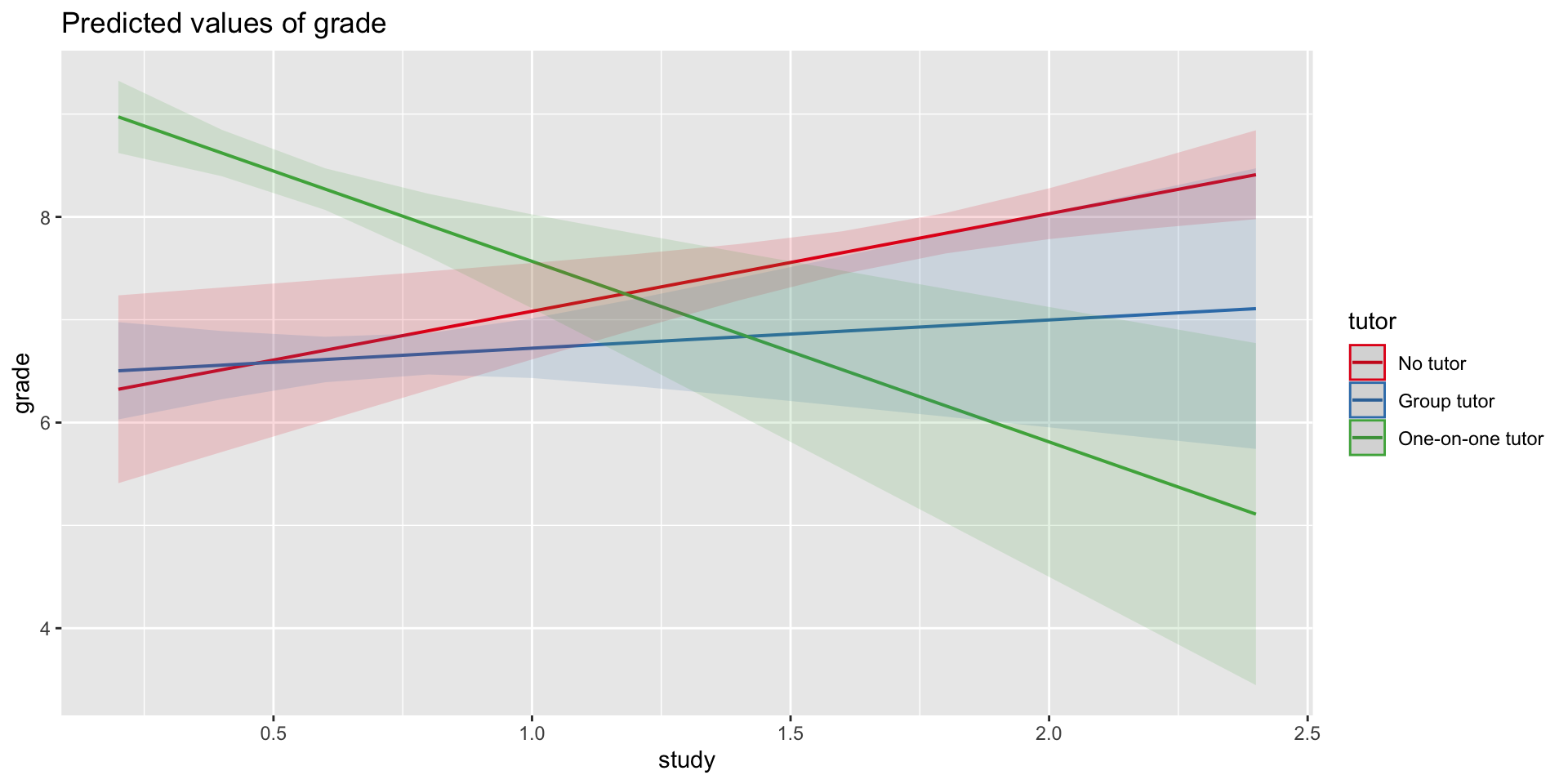
plot_model(mod4, type ="pred", terms =c("study", "tutor"))
emtrends(mod4, pairwise~tutor, var ="study")
$emtrends
 tutor            study.trend    SE df lower.CL upper.CL
 No tutor               0.949 0.297 24    0.336    1.561
 Group tutor            0.275 0.414 24   -0.579    1.128
 One-on-one tutor      -1.756 0.451 24   -2.688   -0.825

Confidence level used: 0.95

$contrasts
 contrast                         estimate    SE df t.ratio p.value
 No tutor - Group tutor              0.674 0.509 24   1.324  0.3962
 No tutor - (One-on-one tutor)       2.705 0.540 24   5.008  0.0001
 Group tutor - (One-on-one tutor)    2.031 0.612 24   3.318  0.0078

P value adjustment: tukey method for comparing a family of 3 estimates
mylist =list(study =c(.5, 1, 2), tutor =c("No tutor", "Group tutor", "One-on-one tutor"))combins =emmeans(mod4, ~tutor*study, at = mylist)contrast(combins, "pairwise", by ="study")
study = 0.5:
 contrast                         estimate    SE df t.ratio p.value
 No tutor - Group tutor             0.0225 0.404 24   0.056  0.9983
 No tutor - (One-on-one tutor)     -1.8377 0.392 24  -4.683  0.0003
 Group tutor - (One-on-one tutor)  -1.8602 0.170 24 -10.930  <.0001

study = 1.0:
 contrast                         estimate    SE df t.ratio p.value
 No tutor - Group tutor             0.3594 0.281 24   1.277  0.4215
 No tutor - (One-on-one tutor)     -0.4853 0.334 24  -1.452  0.3311
 Group tutor - (One-on-one tutor)  -0.8447 0.276 24  -3.059  0.0144

study = 2.0:
 contrast                         estimate    SE df t.ratio p.value
 No tutor - Group tutor             1.0331 0.548 24   1.886  0.1645
 No tutor - (One-on-one tutor)      2.2196 0.682 24   3.257  0.0090
 Group tutor - (One-on-one tutor)   1.1865 0.856 24   1.386  0.3638

P value adjustment: tukey method for comparing a family of 3 estimates