Review & Machine Learning

Last time…

Polynomials
Bootstrapping

Today

Review
Lessons from machine learning

Concept 1: Partial/Semi-partial correlations

A zero-order correlation (\(r\)) assesses the degree covariation between two variables (X and Y). Correlations squared (\(r^2\)) quantify the proportion of variance explained.

Code

library(psych)
data(psych::bfi)
keys.list <- list(
  agree=c("-A1","A2","A3","A4","A5"),
  consc=c("C1","C2","C3","-C4","-C5"),
  extra=c("-E1","-E2","E3","E4","E5"),
  neuro=c("N1","N2","N3","N4","N5"), 
  openn=c("O1","-O2","O3","O4","-O5")) 
  keys <- make.keys(psychTools::bfi,keys.list)  #no longer necessary
 scores <- scoreItems(keys,psychTools::bfi,min=1,max=6)  #using a keys matrix 
bfi_scores = scores$scores %>% as.data.frame()

cor(bfi_scores$agree, bfi_scores$extra, use = "pairwise")

[1] 0.4617888

cor(bfi_scores$agree, bfi_scores$extra, use = "pairwise")^2

[1] 0.2132489

Concept 1: Partial/Semi-partial correlations

In a semi-partial correlation (\(sr\)) assesses the degree covariation between two variables after removing the covariation between one of those variables (X) and a third variable (C). Correlations squared (\(sr^2\)) quantify the proportion of variance explained.

library(ppcor)
spcor.test(bfi_scores$agree, bfi_scores$extra, bfi_scores$neuro)

   estimate       p.value statistic    n gp  Method
1 0.4314948 2.576556e-127  25.29645 2800  1 pearson

spcor.test(bfi_scores$agree, bfi_scores$extra, bfi_scores$neuro)$estimate^2

[1] 0.1861877

Concept 1: Partial/Semi-partial correlations

In a partial correlation (\(pr\)) assesses the degree covariation between two variables after removing the covariation between both primary variables (X and Y) and a third variable (C). Correlations squared (\(pr^2\)) quantify the proportion of variance explained.

pcor.test(bfi_scores$agree, bfi_scores$extra, bfi_scores$neuro)

   estimate      p.value statistic    n gp  Method
1 0.4390438 3.01335e-132  25.84358 2800  1 pearson

pcor.test(bfi_scores$agree, bfi_scores$extra, bfi_scores$neuro)$estimate^2

[1] 0.1927595

Concept 1: Partial/Semi-partial correlations

Sometimes we find that the semi-partial correlation squared is larger than the zero-order.

data = read.csv("https://raw.githubusercontent.com/uopsych/psy612/master/data/vals.csv")
cor(data$V1, data$V2); cor(data$V1, data$V2)^2

[1] 0.4187802

[1] 0.1753769

spcor.test(data$V1, data$V2, data$V3); spcor.test(data$V1, data$V2, data$V3)$estimate^2

   estimate    p.value statistic  n gp  Method
1 0.4749691 0.03987824  2.225389 20  1 pearson

[1] 0.2255957

What’s going on here?

This is a case of suppression. It can happen when our predictors are highly correlated, but our control variable is not associated with the outcome:

cor(data) %>%  round(2)

     V1   V2   V3
V1 1.00 0.42 0.00
V2 0.42 1.00 0.47
V3 0.00 0.47 1.00

It can also happen when there is an inconsistency of signs. Recall the formula:

\[sr = \frac{r_{Y1}- r_{Y2}r_{12}}{1-r_{12}^2}\]

Concept 2: Interpreting SS in Factorial ANOVA

Hypothetical data on the combined efficacy of SSRIs and DBT.

data = read.csv("https://raw.githubusercontent.com/uopsych/psy612/master/data/depresssion.csv")
psych::describe(data, fast = T)

           vars  n mean   sd min  max range   se
drug          1 40  NaN   NA Inf -Inf  -Inf   NA
therapy       2 40  NaN   NA Inf -Inf  -Inf   NA
depression    3 40 3.34 1.11   1    5     4 0.18

table(data$drug, data$therapy)

         
          DBT No therapy
  No drug  10         10
  SSRI     10         10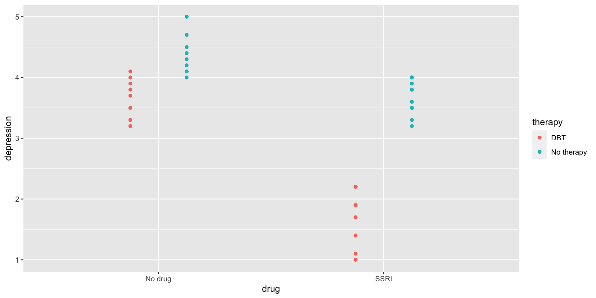

ggplot(data, aes(x = drug, y = depression, color = therapy)) +
  geom_point(position = position_dodge(.5))

model = lm(depression ~ drug*therapy, data = data)
anova(model)

Analysis of Variance Table

Response: depression
             Df Sum Sq Mean Sq F value    Pr(>F)    
drug          1 19.044 19.0440 139.858 5.863e-14 ***
therapy       1 20.164 20.1640 148.083 2.561e-14 ***
drug:therapy  1  3.721  3.7210  27.327 7.484e-06 ***
Residuals    36  4.902  0.1362                      
---
Signif. codes:  0 '***' 0.001 '**' 0.01 '*' 0.05 '.' 0.1 ' ' 1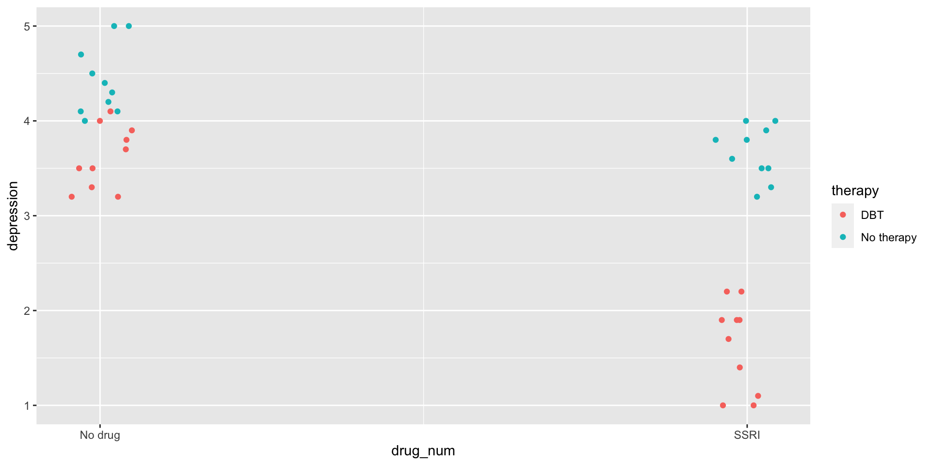

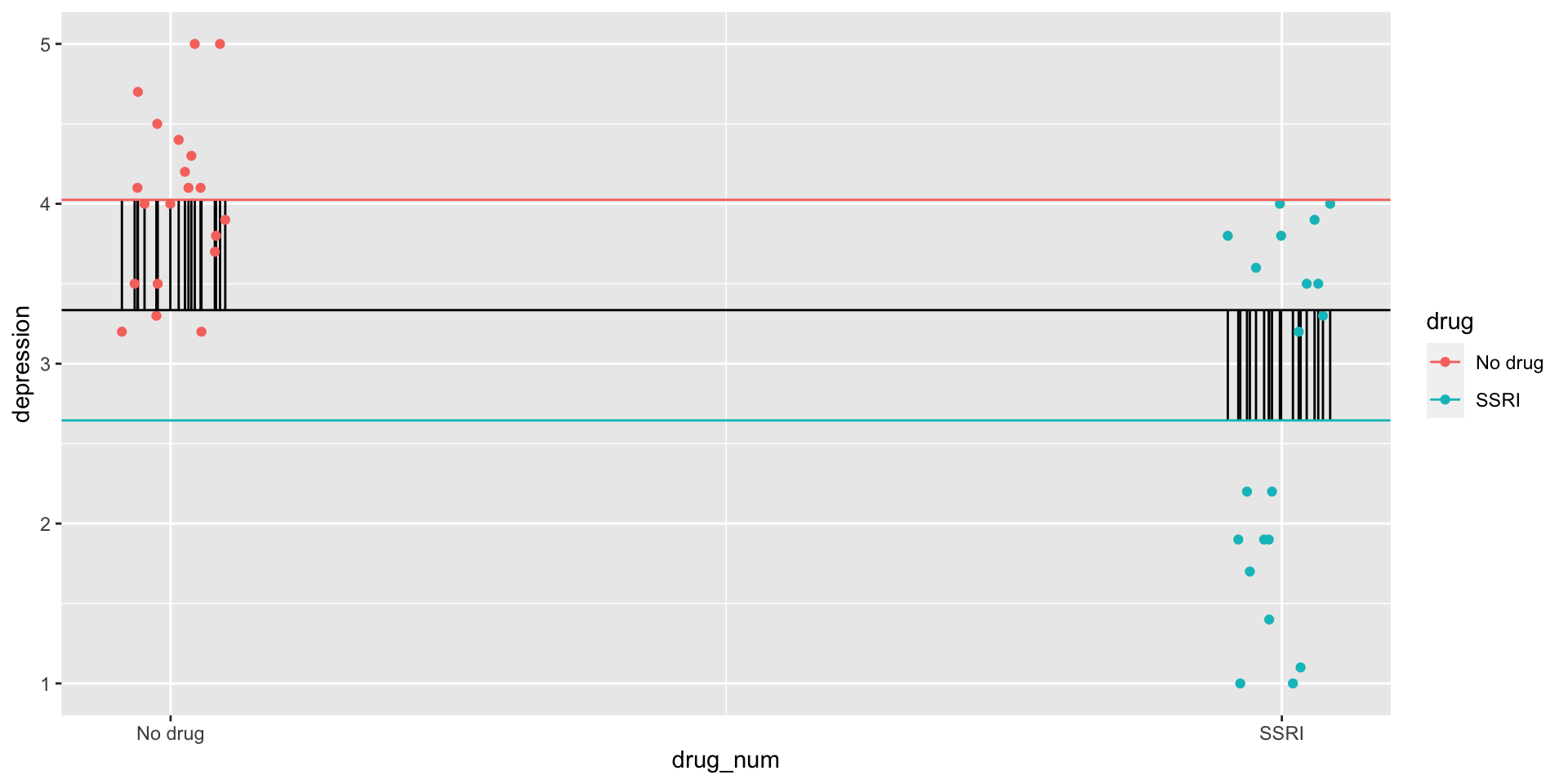
Variability between drug conditions

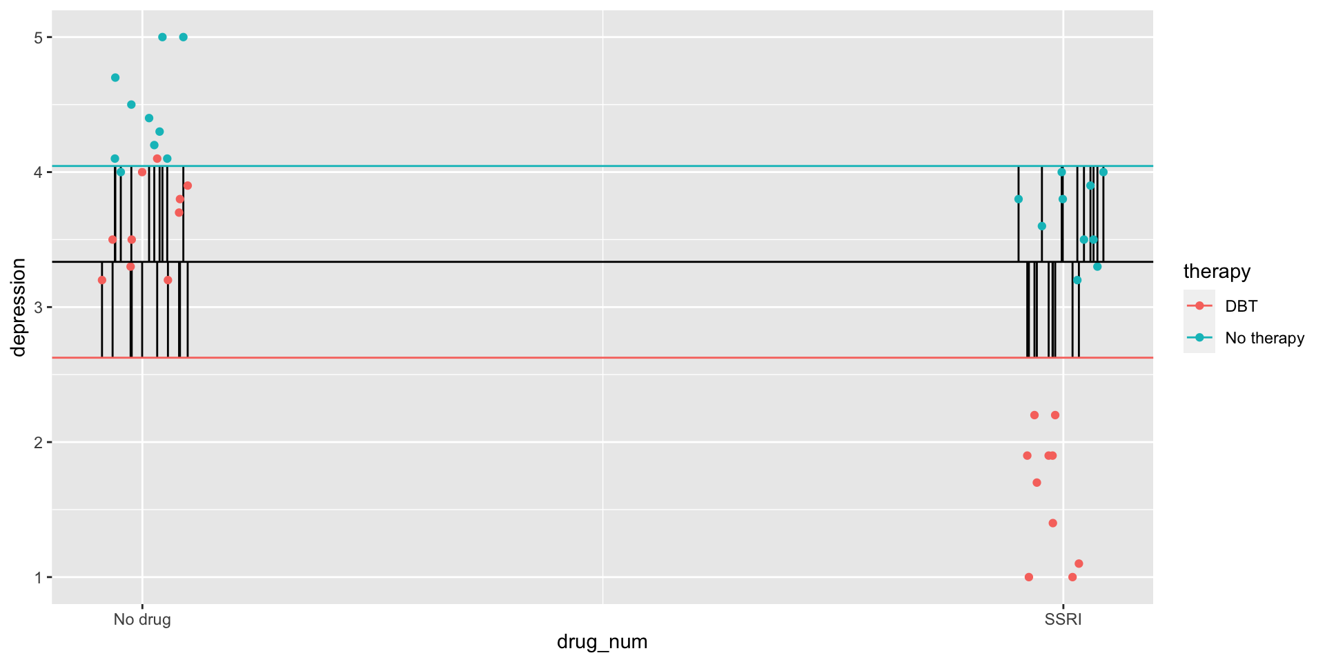
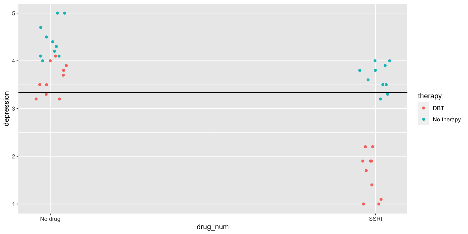
Variability between therapy conditions

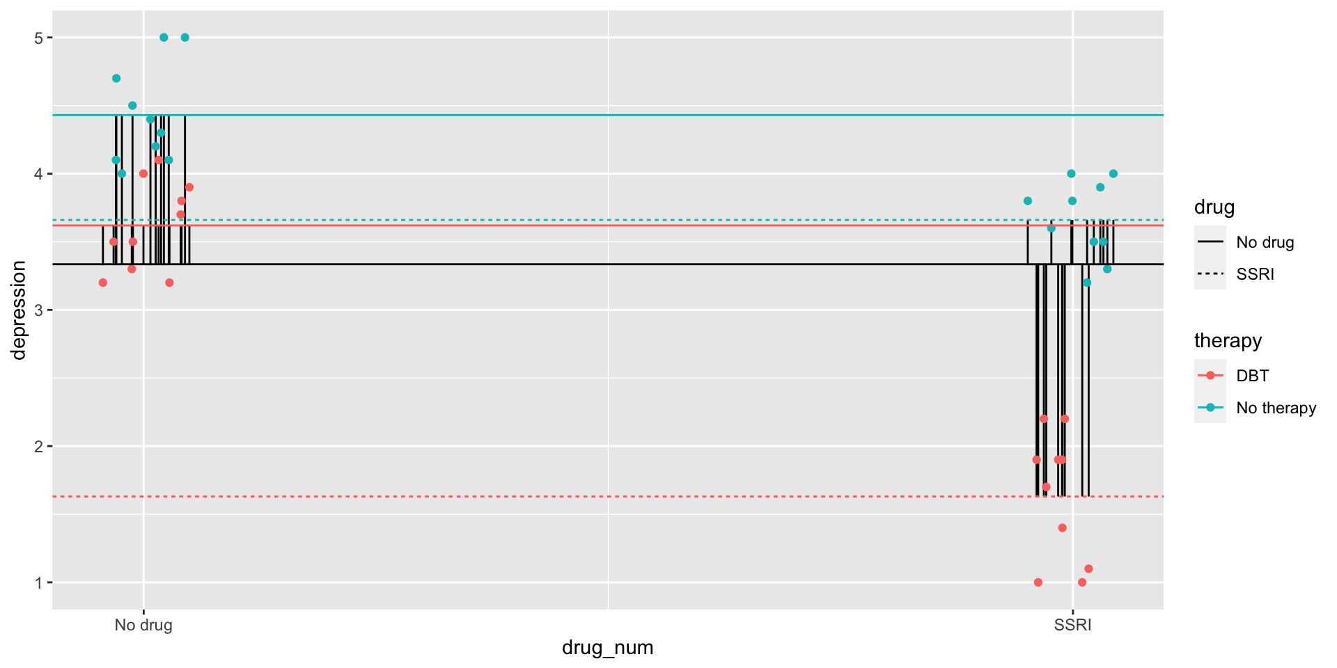
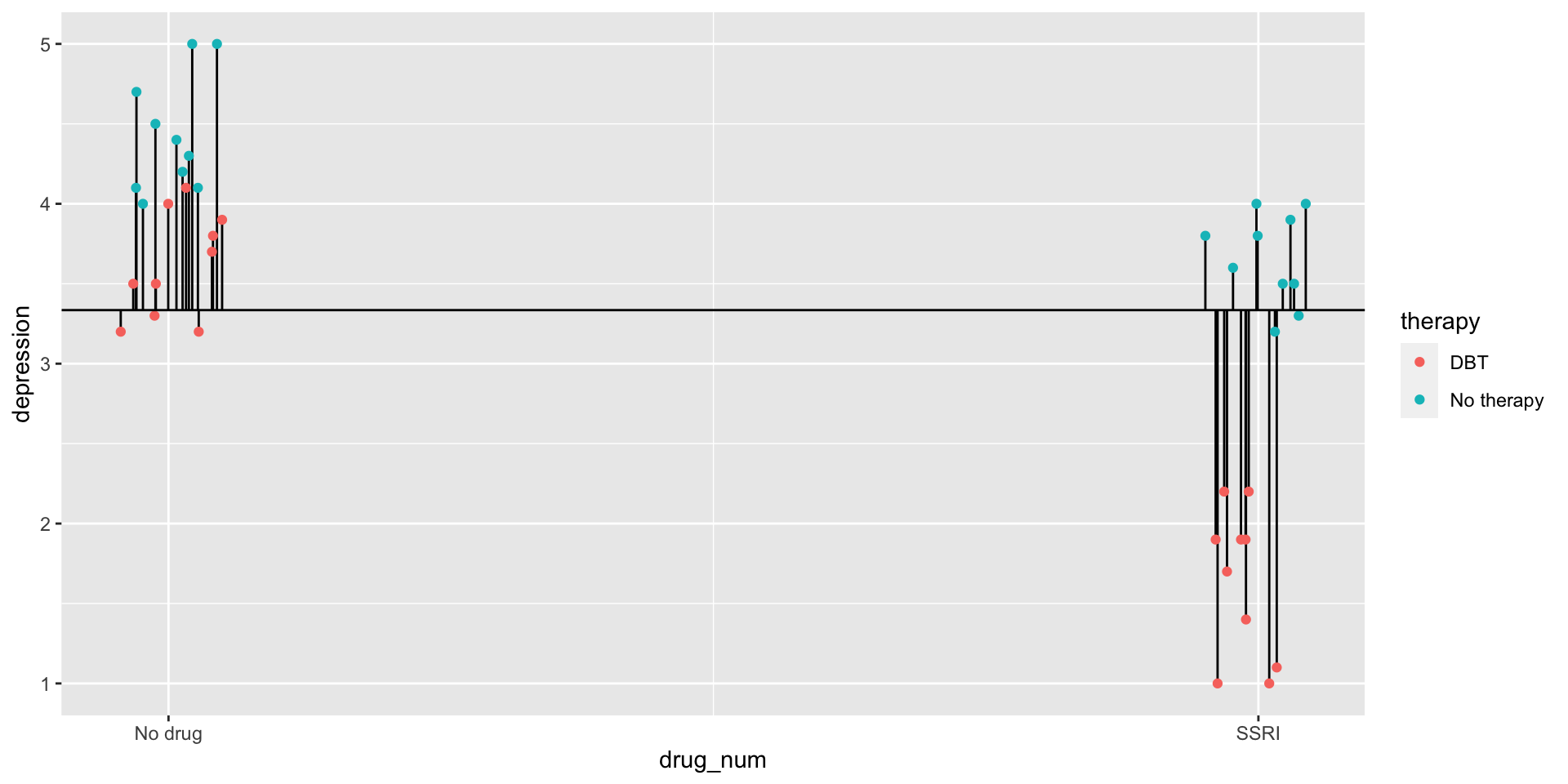
Variability between cells

model = lm(depression ~ drug*therapy, data = data)
anova(model)

Analysis of Variance Table

Response: depression
             Df Sum Sq Mean Sq F value    Pr(>F)    
drug          1 19.044 19.0440 139.858 5.863e-14 ***
therapy       1 20.164 20.1640 148.083 2.561e-14 ***
drug:therapy  1  3.721  3.7210  27.327 7.484e-06 ***
Residuals    36  4.902  0.1362                      
---
Signif. codes:  0 '***' 0.001 '**' 0.01 '*' 0.05 '.' 0.1 ' ' 1

Concept 3: Checking assumptions of Factorial ANOVAs

Start with the 6 assumption of regression models

No measurement error
Correct form
Correct model
Homoscedasticity
Independence
Normality of residuals

Concept 3: Checking assumptions of Factorial ANOVAs

Start with the 6 assumption of regression models

No measurement error
~~Correct form~~
Correct model
Homoscedasticity
Independence
Normality of residuals

Homoscedasticity

data %>% 
  group_by(therapy, drug) %>% 
  summarise(m = mean(depression, s = sd(depression)))

# A tibble: 4 × 3
# Groups:   therapy [2]
  therapy    drug        m
  <chr>      <chr>   <dbl>
1 DBT        No drug  3.62
2 DBT        SSRI     1.63
3 No therapy No drug  4.43
4 No therapy SSRI     3.66

car::leveneTest(depression ~ drug*therapy, data = data)

Levene's Test for Homogeneity of Variance (center = median)
      Df F value Pr(>F)
group  3  0.9427 0.4302
      36

Lessons from machine learning

Yarkoni and Westfall (2017) describe the goals of explanation and prediction in science. - Explanation: describe causal underpinnings of behaviors/outcomes - Prediction: accurately forecast behaviors/outcomes

In some ways, these goals work in tandem. Good prediction can help us develop theory of explanation and vice versa. But, statistically speaking, they are in tension with one another: statistical models that accurately describe causal truths often have poor prediction and are complex; predictive models are often very different from the data-generating processes.

Yarkoni and Westfall (2017)

Overfitting: mistakenly fitting sample-specific noise as if it were signal - OLS models tend to be overfit because they minimize error for a specific sample

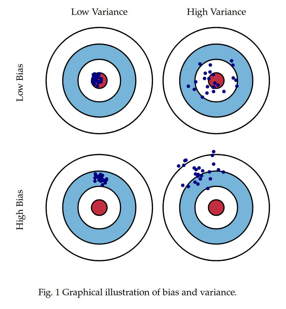
Bias: systematically over or under estimating parameters

Variance: how much estimates tend to jump around

Yarkoni and Westfall (2017)

Big Data

Reduce the likelihood of overfitting – more data means less error

Cross-validation

Is my model overfit?

Regularization

Constrain the model to be less overfit (and more biased)

Big Data Sets

“Every pattern that could be observed in a given dataset reflects some… unknown combination of signal and error” (page 1104).

Error is random, so it cannot correlate with anything; as we aggregate many pieces of information together, we reduce error.

Thus, as we get bigger and bigger datasets, the amount of error we have gets smaller and smaller

Cross-validation

Cross-validation is a family of techniques that involve testing and training a model on different samples of data.

Replication
Hold-out samples
K-fold
- Split the original dataset into 2(+) datasets, train a model on one set, test it in the other
Recycle: each dataset can be a training AND a testing; average model fit results to get better estimate of fit
- Can split the dataset into more than 2 sections

library(here)
stress.data = read.csv(here("data/stress.csv"))
library(psych)
describe(stress.data, fast = T)

        vars   n  mean    sd  min    max  range   se
id         1 118 59.50 34.21 1.00 118.00 117.00 3.15
Anxiety    2 118  7.61  2.49 0.70  14.64  13.94 0.23
Stress     3 118  5.18  1.88 0.62  10.32   9.71 0.17
Support    4 118  8.73  3.28 0.02  17.34  17.32 0.30
group      5 118   NaN    NA  Inf   -Inf   -Inf   NA

model.lm = lm(Stress ~ Anxiety*Support*group, 
              data = stress.data)
summary(model.lm)$r.squared

[1] 0.4126943

Example: 10-fold cross validation

# new package!
library(caret)
# set control parameters
ctrl <- trainControl(method="cv", number=10)
# use train() instead of lm()
cv.model <- train(Stress ~ Anxiety*Support*group, 
               data = stress.data, 
               trControl=ctrl, # what are the control parameters
               method="lm") # what kind of model
cv.model

Example: 10-fold cross validation

Linear Regression 

118 samples
  3 predictor

No pre-processing
Resampling: Cross-Validated (10 fold) 
Summary of sample sizes: 106, 106, 106, 106, 106, 106, ... 
Resampling results:

  RMSE      Rsquared   MAE     
  1.550296  0.3307817  1.246434

Tuning parameter 'intercept' was held constant at a value of TRUE

Regularization

Penalizing a model as it grows more complex.

Usually involves shrinking coefficient estimates – the model will fit less well in-sample but may be more predictive

lasso regression: balance minimizing sum of squared residuals (OLS) and minimizing smallest sum of absolute values of coefficients

coefficients are more biased (tend to underestimate coefficients) but produce less variability in results

See here for a tutorial.

NHST no more

Once you’ve imposed a shrinkage penalty on your coefficients, you’ve wandered far from the realm of null hypothesis significance testing. In general, you’ll find that very few machine learning techniques are compatible with probability theory (including Bayesian), because they’re focused on different goals. Instead of asking, “how does random chance factor into my result?”, machine learning optimizes (out of sample) prediction. Both methods explicitly deal with random variability. In NHST and Bayesian probability, we’re trying to estimate the degree of randomness; in machine learning, we’re trying to remove it.

Summary: Yarkoni and Westfall (2017)

Big Data

Reduce the likelihood of overfitting – more data means less error

Cross-validation

Is my model overfit?

Regularization

Constrain the model to be less overfit

Next time…

PSY 613 with Elliot Berkman!

(But first take the final quiz.)