Bonus lecture

Last time

Paired-samples t-tests

aka one-sample t-tests on difference scores

library(tidyverse)

Today

Repeated measures
Intro to text analysis
Bootstrapping?

Repeated Measures

How does the number of trials per participant affect statistical power?
Can more trials compensate for fewer participants?
How do we analyze experiments with multiple trials per participant?

Key Concepts

In cognitive experiments, we have:
- Multiple participants (n)
- Multiple trials per participant (k)
- Two or more conditions
- Each trial produces a measurement
Multiple trials can:
1. Improve measurement precision
2. Reduce within-subject variability
3. Increase reliability

Simulation: Effect of Trials

(Function to simulate experiment here)

Code

simulate_cognitive_experiment <- function(
    n_participants = 20,    # number of participants
    n_trials = 50,         # trials per condition per participant
    true_effect = 0.5,     # mean difference between conditions
    participant_sd = 0.25,   # between-participant variability
    trial_sd = 1.0,        # within-participant (trial) variability
    seed = 123             # for reproducibility
) {
  
  set.seed(seed)
  
  # Generate participant random effects (individual differences)
  participant_effects <- rnorm(n_participants, mean = 0, sd = participant_sd)
  
  # Create a data frame with all combinations of participants and trials
  experiment_data <- expand_grid(
    participant = 1:n_participants,
    trial = 1:n_trials,
    condition = c("A", "B")
  ) %>%
    # Add participant-level random effects
    mutate(
      participant_effect = rep(participant_effects, each = n_trials * 2),
      # Add condition effect (only for condition B)
      condition_effect = if_else(condition == "B", true_effect, 0),
      # Generate trial-level noise
      trial_noise = rnorm(n(), mean = 0, sd = trial_sd),
      # Compute response time (or other DV)
      response = 0.5 + participant_effect + condition_effect + trial_noise
    ) %>%
    # Reorder columns for clarity
    select(participant, condition, trial, response)
  
  return(experiment_data)
}

# Generate example data
data <- simulate_cognitive_experiment(
  n_participants = 20,
  n_trials = 100,
  true_effect = 0.5,
  participant_sd = 0.25,
  trial_sd = 1.0
)

# View first few rows
data

# A tibble: 4,000 × 4
   participant condition trial response
         <int> <chr>     <int>    <dbl>
 1           1 A             1   -0.708
 2           1 B             1    0.642
 3           1 A             2   -0.666
 4           1 B             2    0.131
 5           1 A             3   -0.265
 6           1 B             3   -0.827
 7           1 A             4    1.20 
 8           1 B             4    1.01 
 9           1 A             5   -0.778
10           1 B             5    2.11 
# ℹ 3,990 more rows

# Basic summary statistics
data %>%
  group_by(condition) %>%
  summarise(
    mean_rt = mean(response),
    sd_rt = sd(response),
    n_trials = n()
  )

# A tibble: 2 × 4
  condition mean_rt sd_rt n_trials
  <chr>       <dbl> <dbl>    <int>
1 A           0.544  1.02     2000
2 B           1.04   1.01     2000

# Participant-level summary
data %>%
  group_by(participant, condition) %>%
  summarise(
    mean_rt = mean(response),
    sd_rt = sd(response),
    n_trials = n(),
    .groups = "drop"
  )

# A tibble: 40 × 5
   participant condition mean_rt sd_rt n_trials
         <int> <chr>       <dbl> <dbl>    <int>
 1           1 A           0.345 0.935      100
 2           1 B           0.842 0.967      100
 3           2 A           0.562 0.929      100
 4           2 B           0.853 1.03       100
 5           3 A           1.07  1.04       100
 6           3 B           1.27  0.914      100
 7           4 A           0.558 1.01       100
 8           4 B           0.991 1.03       100
 9           5 A           0.561 1.02       100
10           5 B           1.12  1.14       100
# ℹ 30 more rows

# Calculate effect size for each participant
participant_effects <- data %>%
  group_by(participant, condition) %>%
  summarise(
    mean_rt = mean(response),
    .groups = "drop"
  ) %>%
  pivot_wider(
    names_from = condition,
    values_from = mean_rt
  ) %>%
  mutate(effect_size = B - A)

# A tibble: 20 × 4
   participant      A     B effect_size
         <int>  <dbl> <dbl>       <dbl>
 1           1  0.345 0.842       0.497
 2           2  0.562 0.853       0.291
 3           3  1.07  1.27        0.200
 4           4  0.558 0.991       0.433
 5           5  0.561 1.12        0.564
 6           6  0.977 1.38        0.401
 7           7  0.597 1.15        0.555
 8           8  0.139 0.881       0.742
 9           9  0.315 0.911       0.596
10          10  0.395 1.01        0.620
11          11  0.752 1.17        0.416
12          12  0.543 0.947       0.405
13          13  0.662 1.17        0.510
14          14  0.488 0.975       0.486
15          15  0.480 0.927       0.447
16          16  0.845 1.38        0.534
17          17  0.562 1.20        0.634
18          18 -0.107 0.688       0.796
19          19  0.582 0.992       0.410
20          20  0.561 0.940       0.379

# Aggregating across different trial numbers
participant_effects20 <- data %>%
  filter(trial <= 20) %>% 
  group_by(participant, condition) %>%
  summarise(
    mean_rt = mean(response),
    .groups = "drop"
  ) %>%
  pivot_wider(
    names_from = condition,
    values_from = mean_rt
  ) %>%
  mutate(effect_size = B - A)

# A tibble: 20 × 4
   participant       A     B effect_size
         <int>   <dbl> <dbl>       <dbl>
 1           1  0.238  1.04       0.800 
 2           2  0.627  0.696      0.0686
 3           3  1.15   1.30       0.158 
 4           4  0.324  1.05       0.721 
 5           5  0.524  1.11       0.583 
 6           6  1.05   1.58       0.529 
 7           7  0.590  1.21       0.616 
 8           8  0.0702 0.980      0.910 
 9           9  0.127  1.07       0.947 
10          10  0.321  0.900      0.579 
11          11  0.904  1.40       0.495 
12          12  0.413  0.736      0.322 
13          13  0.507  1.24       0.729 
14          14  0.901  0.945      0.0440
15          15  0.401  1.12       0.715 
16          16  0.812  1.14       0.332 
17          17  0.568  1.38       0.809 
18          18 -0.146  0.841      0.987 
19          19  0.610  1.15       0.538 
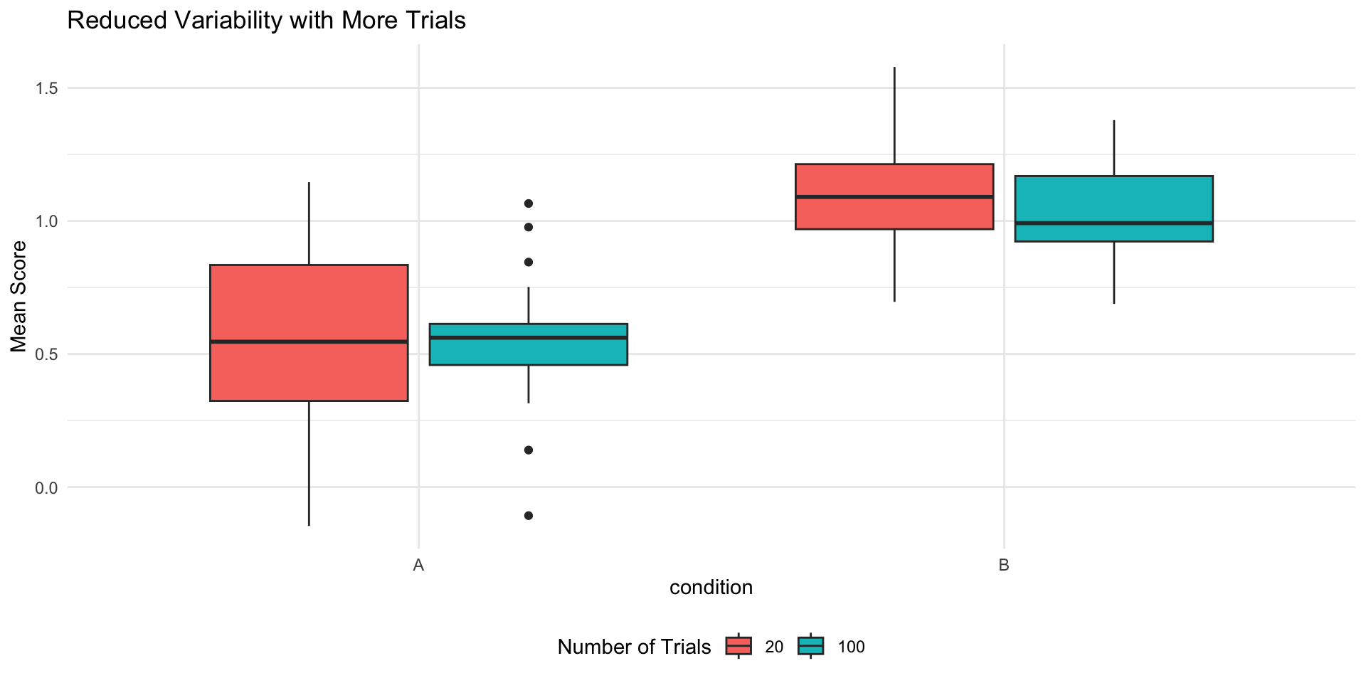
20          20  0.955  0.977      0.0217

t.test(participant_effects20$A, participant_effects20$B, 
       paired = TRUE)$statistic

        t 
-8.090232

t.test(participant_effects$A, participant_effects$B, 
       paired = TRUE)$statistic

        t 
-15.56358

Why More Trials Help

Law of Large Numbers

Individual trial measurements are noisy
Mean of many trials is more stable
Reduces measurement error

Standard Error Formula

SE = σ / √n
More trials → smaller SE of participant means
Smaller SE → More power

Code

participant_effects %>% 
  mutate(Trials = 100) %>% 
  full_join(
    mutate(participant_effects20, Trials = 20)
  ) %>% 
  pivot_longer(cols = c("A", "B"),
               names_to = "condition",
               values_to = "avg_response") %>% 
  ggplot(., aes(x = condition, 
                     y = avg_response, 
                     fill = as.factor(Trials))) +
  geom_boxplot() +
  labs(title = "Reduced Variability with More Trials", 
       y = "Mean Score", 
       fill = "Number of Trials") +
  theme_minimal() +
  theme(legend.position = "bottom")

Practical Guidelines

More trials generally help, but with diminishing returns
Consider:
- Participant fatigue
- Practice effects
- Time constraints
- Resource limitations

Analysis Approaches

Summary by Dan McNeish

Participant-level Analysis
- Average trials for each participant
- Run paired t-test on participant means
- Simple but may lose information
Multilevel modeling
- Use all information
- Especially useful when interested in individual differences
Clustered errors and GEE
- Don’t care about individual differences
Fixed effects models
- Useful when relevant contextual factors are not measured

Coming Soon (PSY 613)…

Mixed-effects models
- Account for trial-level variation
- Handle missing data
- Model individual differences
Power analysis for repeated measures

library(lme4)
lmer(response ~ 1 + condition + (1|participant),
     data = data) %>% 
  summary()

Linear mixed model fit by REML ['lmerMod']
Formula: response ~ 1 + condition + (1 | participant)
   Data: data

REML criterion at convergence: 11358.8

Scaled residuals: 
    Min      1Q  Median      3Q     Max 
-3.2348 -0.6633 -0.0035  0.6758  3.4111 

Random effects:
 Groups      Name        Variance Std.Dev.
 participant (Intercept) 0.0416   0.2039  
 Residual                0.9888   0.9944  
Number of obs: 4000, groups:  participant, 20

Fixed effects:
            Estimate Std. Error t value
(Intercept)  0.54415    0.05074   10.72
conditionB   0.49573    0.03145   15.77

Correlation of Fixed Effects:
           (Intr)
conditionB -0.310

Text analysis

Data came from a study of parents of young children, collected during 2020.

Parents answered the question: “How do you feel about the COVID-19 vaccine in terms of its safety and effectiveness, and what are your plans in terms of whether or not to get it?”

# install.packages(c("textdata", "tidytext", "wordcloud"))
library(tidytext)
library(textdata)
library(wordcloud)
rapid = read_csv("https://raw.githubusercontent.com/uopsych/psy611/refs/heads/master/data/rapid_short.csv")

Data Preparation

Let’s examine and clean our text data:

# Look at the structure of our data
glimpse(rapid)

Rows: 6,554
Columns: 7
$ ...1         <dbl> 23435, 23436, 23437, 23439, 23440, 23444, 23445, 23451, 2…
$ CaregiverID  <chr> "R3ID00020", "R3ID00032", "R3ID00032", "R3ID00036", "R3ID…
$ StartDate    <dttm> 2021-06-11 08:15:52, 2021-06-09 10:59:01, 2021-11-10 09:…
$ CaregiverAge <lgl> NA, NA, NA, NA, NA, NA, NA, NA, NA, NA, NA, NA, NA, NA, N…
$ DEMO.006.a   <lgl> NA, NA, NA, NA, NA, NA, NA, NA, NA, NA, NA, NA, NA, NA, N…
$ DEMO.014     <dbl> NA, NA, NA, NA, NA, NA, NA, NA, NA, NA, NA, NA, NA, NA, N…
$ HEALTH.030   <chr> "I am not planning on it right now but i am open to the f…

Cleaning text requires the use of “regular expressions.” This is like a sub-dialect of coding. The website regex101.com is very useful for navigating this code, but of course, AI is great too.

# Create a clean text column
rapid_clean <- rapid %>%
  mutate(
    response = HEALTH.030,
    # Convert to lowercase
    response = tolower(response),
    # Remove punctuation
    response = str_remove_all(response, "\\?"),
    response = str_replace_all(response, "[[:punct:]]", " "),
    # Remove extra whitespace
    response = str_squish(response)
  )

head(rapid_clean$response) # show first few responses

[1] "i am not planning on it right now but i am open to the future"                                                  
[2] "i dont feel it is safe yet or ready"                                                                            
[3] "im not sure about the vaccine and its effectiveness im still weary and havent decided on taking the vaccine yet"
[4] "i dont feel like it works i had to get it for work"                                                             
[5] "i already got both doses"                                                                                       
[6] "i got it"

Breaking Text into Words

We’ll use tidytext to tokenize our responses:

words_df <- rapid_clean %>%
  unnest_tokens(word, response) %>%
  # Remove stop words
  anti_join(stop_words)

# View most common words
words_df %>%
  count(word, sort = TRUE) %>%
  slice_head(n = 10) %>%
  knitr::kable()

word	n
vaccine	1789
safe	1747
vaccinated	1457
feel	1210
received	976
effective	952
covid	514
booster	463
plan	460
children	449

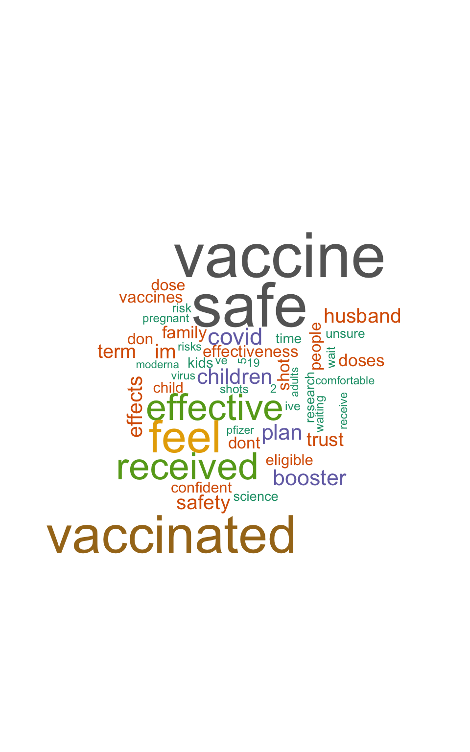
Visualizing Common Words

Let’s create a word cloud:

words_df %>%
  count(word) %>%
  with(wordcloud(word, n, 
                max.words = 50, 
                colors = brewer.pal(8, "Dark2")))

Finding Themes: Bigrams

Let’s look at word pairs to understand context better:

Code

bigrams_df <- rapid_clean %>%
  unnest_tokens(bigram, response, token = "ngrams", n = 2) %>%
  separate(bigram, c("word1", "word2"), sep = " ") %>% 
  filter(!word1 %in% stop_words$word,
         !word2 %in% stop_words$word) %>%
  filter(!is.na(word1)) %>%
  filter(!is.na(word2))

# View top bigrams
bigrams_df %>%
  unite(bigram, word1, word2, sep = " ") %>%
  count(bigram, sort = TRUE) %>%
  slice_head(n = 10) %>%
  knitr::kable()

bigram	n
term effects	154
covid 19	118
feel confident	65
19 vaccine	47
dont feel	46
dont trust	44
covid vaccine	43
feel comfortable	43
children vaccinated	41
feel safe	39

Sentiment Analysis

Let’s analyze the emotional content of responses:

get_sentiments("bing") %>%
  sample_n(10)

# A tibble: 10 × 2
   word          sentiment
   <chr>         <chr>    
 1 shark         negative 
 2 awsome        positive 
 3 irrepressible negative 
 4 humiliation   negative 
 5 disgruntled   negative 
 6 preferably    positive 
 7 comforting    positive 
 8 immobilized   negative 
 9 bored         negative 
10 eye-catching  positive

Sentiment Analysis

# Add sentiment scores
sentiment_df <- words_df %>% 
  inner_join(get_sentiments("bing")) %>% 
  count(CaregiverID, StartDate, sentiment) %>%
  pivot_wider(names_from = sentiment, 
              values_from = n, 
              values_fill = 0) %>%
  mutate(sentiment_score = positive - negative)

sentiment_df

# A tibble: 4,070 × 5
   CaregiverID StartDate           positive negative sentiment_score
   <chr>       <dttm>                 <int>    <int>           <int>
 1 R3ID00032   2021-06-09 10:59:01        2        0               2
 2 R3ID00032   2021-11-10 09:57:51        1        1               0
 3 R3ID00049   2021-12-10 08:17:19        1        0               1
 4 R3ID00083   2021-11-14 09:11:26        0        1              -1
 5 R3ID00084   2021-06-11 10:58:56        1        0               1
 6 R3ID00084   2021-10-13 09:21:12        1        0               1
 7 R3ID00117   2021-12-08 10:30:31        0        1              -1
 8 R3ID00166   2021-03-17 22:15:04        1        0               1
 9 R3ID00168   2021-12-08 10:13:24        1        0               1
10 R3ID00188   2021-10-14 09:17:07        1        0               1
# ℹ 4,060 more rows

Sentiment Analysis

Code

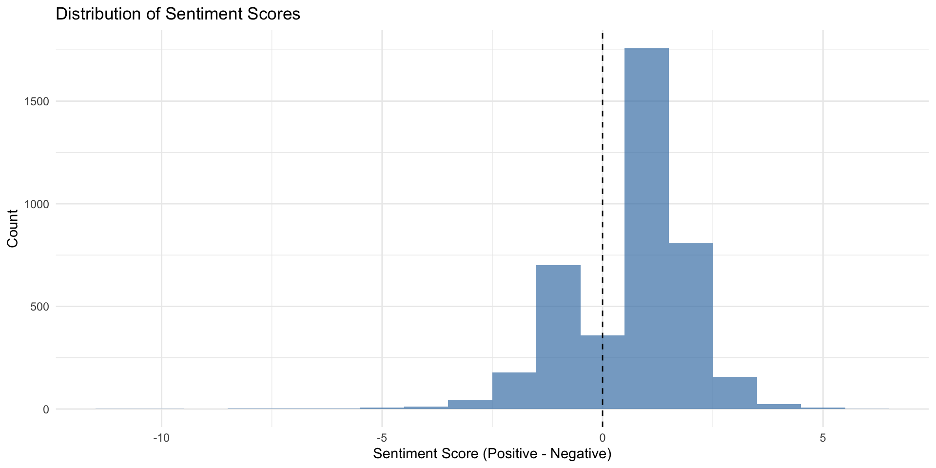
# View distribution of sentiment
ggplot(sentiment_df, aes(x = sentiment_score)) +
  geom_histogram(binwidth = 1, fill = "steelblue", alpha = 0.7) +
  geom_vline(aes(xintercept = 0), linetype = "dashed") +
  labs(title = "Distribution of Sentiment Scores",
       x = "Sentiment Score (Positive - Negative)",
       y = "Count") +
  theme_minimal()

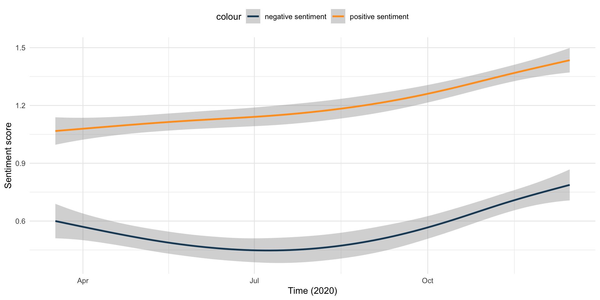
Does sentiment change over time?

Code

sentiment_df %>% 
  ggplot(aes(x = StartDate)) +
  geom_smooth(aes(y = positive, color = "positive sentiment")) +
  geom_smooth(aes(y = negative, color = "negative sentiment")) +
  scale_color_manual(values = c("#1B4965", "#FF9F1C")) +
  labs(
    x = "Time (2020)",
    y = "Sentiment score"
  ) +
  theme_minimal() +
  theme(legend.position = "top")

Key Findings

Most common words reveal attitudes about vaccine safety and effectiveness
Common bigrams show personal experiences (“already got”, “fully vaccinated”)
Sentiment analysis reveals mixed but generally positive attitudes

Resources for Learning More

tidytext documentation: https://www.tidytextmining.com/
Text Mining with R (free online book)
UPenn Library
Michael Clark workshop